
Abstract
It is common for suppliers operating in batch‐production mode to deal with patient and impatient customers. This paper considers inventory models in which a supplier provides alternative lead times to its customers: a short or a long lead time. Orders from patient customers can be taken by the supplier and included in the next production cycle, while orders from impatient customers have to be satisfied from the on‐hand inventory. We denote the action to commit one unit of on‐hand inventory to patient or impatient customers as the inventory‐commitment decision, and the initial inventory stocking as the inventory‐replenishment decision. We first characterize the optimal inventory‐commitment policy as a threshold type, and then prove that the optimal inventory‐replenishment policy is a base‐stock type. Then, we extend our analysis to models to consider cases of a multi‐cycle setting, a supply‐capacity constraint, and the on‐line charged inventory‐holding cost. We also evaluate and compare the performances of the optimal inventory‐commitment policy and the inventory‐rationing policy. Finally, to further investigate the benefits and pitfalls of introducing an alternative lead‐time choice, we use the customer‐choice model to study the demand gains and losses, known as demand‐induction and demand‐cannibalization effects, respectively.
1. Introduction
A supplier/manufacturer operating in batch‐production mode may deal with two kinds of customers: patient (slow) and impatient (fast) customers. Impatient customers have a shorter operational cycle than the supplier, and patient customers have a longer operational cycle than the supplier. For example, H&M and Zara are fast fashion retailers. In addition to their talented instincts about fashion trends and their quick response programs with shorter operational cycles, it is their acclaimed achievements in cutting lead times that have led to their phenomenal success. In contrast, traditional retailers such as Gap may serve less trendy market segments. These traditional retailers may also be large, and thus may have fewer incentives and more difficulties in adopting quick response programs (Caro and Martínez‐de‐Albéniz 2008). Although they have certain trendy elements, such companies operate with a longer operational cycle. Therefore, suppliers who serve both Zara and Gap have to deal with slow and fast orders together. Orders taken by suppliers from slow customers can be included in the next production cycle, whereas orders from fast customers have to be satisfied from the on‐hand inventory.
A renowned management concept in the service industry is the notion of revenue management, wherein capacities are reserved for possible high‐margin customers. In the manufacturing sector, order promising, or available to promise (ATP), is the communication process between a customer and a supplier for a reliable delivery date. In addition, modern manufacturing companies rely on their enterprise resource planning systems or advanced planning systems (APS) to provide real‐time order delivery information. ATP has a powerful order‐promising feature that provides forward‐looking visibility of what can be produced and promised, as well as maximum production flexibility by delaying the commitment of a particular end item as long as possible.
In this paper, we define a long lead‐time customer as one that pays a lower price and accepts a set of two alternative lead‐times so that the supplier can choose the delivery time at its convenience. We define a short lead‐time customer as one that pays a higher price and requires immediate delivery. Note that the supplier has its own production lead time. In this paper, we assume that the production lead time is shorter than the lead time of long lead‐time customers, but longer than the lead time of short lead‐time customers. Therefore, at the time an order is placed, the short lead‐time customer is informed if the order is fulfilled immediately; whereas the long lead‐time customer is informed whether the order is fulfilled immediately or is going to be fulfilled in the next cycle.
1.1. Literature Review
The most relevant literature concerns inventory systems that serve multiple‐customer classes. For periodic‐review inventory models, a representative result is known as an inventory‐rationing policy that defines a static threshold for each customer class which represents the maximum number of orders to be reserved for the corresponding class. Veinott (1965) first considers the problem of multiple demand classes and introduces the concept of rationing. Topkis (1968) further refines the inventory‐rationing policy in which he divides the replenishment cycle into a finite number of intervals. On‐hand inventory is allocated to each time interval. At the end of a given time interval, orders are accepted or backlogged in the backlog case (lost in the lost‐sale case). Kaplan (1969) independently obtains the same inventory‐rationing policy for the backlog case as does Topkis (1968), but without considering the inventory‐replenishment issue. Cattani and Souza (2002) study an inventory system with two lead‐time requirement customers, and they numerically compare the performances of an inventory‐rationing policy and the first‐come first‐served policy. Jang (2000) and Jang and Kim (2006) study a newsvendor‐type model that considers two classes of customers with different waiting costs. They also consider production, inventory rationing, and distribution decisions. Frank et al. (2003) characterize the optimal policies in a periodic‐review inventory system to serve deterministic and stochastic demands, in which the deterministic demand must be satisfied and inventory replenishment has a set‐up cost. An inventory‐rationing policy is used to reserve inventory for committed deterministic demand. Ding et al. (2006) develop an inventory‐rationing model that incorporates a price‐discount mechanism and allows inventory backlogging. Recently, Duran et al. (2007) study a multi‐period inventory system in which customers are differentiated by lead‐time requirements. At the end of each period, after the impatient and patient customer demand is revealed, the supplier decides the amount of inventory to reserve, the amount of patient customers to backlog, and the next‐period inventory replenishment. With this setting, they show that, in any period, the rejected patient customers and the backlogged patient customers cannot co‐exist. They obtain an (S, R, B) policy in which S, R, and B are the order‐up‐to, reserve‐up‐to, and backlog‐up‐to levels. To serve both transaction and contractual customers, Gupta and Wang (2007) study periodic‐review infinite‐horizon inventory models in the make‐to‐order and make‐to‐stock/make‐to‐order environments. They prove that a threshold policy is optimal for the make‐to‐order mode and that a two‐critical‐number policy performs well for the make‐to‐stock/make‐to‐order mode.
Compared with these periodic‐review inventory models with inventory rationing, the key difference in our model is that it allocates goods upon the arrival of a customer (in real time). This is of practical interest, because, as also pointed out by Ding et al. (2006), “in most practical cases, demand arrives according to a continuous‐time stochastic process during a period and firms are required to respond to demands immediately.” As analyzed in our model, the evolution of inventory dynamics (the inventory state) depends on the realization sequence of both short and long lead‐time customers and the admission control deployed. In contrast, these inventory‐rationing models dispatch goods to customers at the end of a period when ALL demands are realized. Therefore, the customer‐arrival sequence does not matter, and the evolution of inventory dynamics depends only on the cumulative demand.
For continuous‐review inventory models, Deshpande et al. (2003) develop a model for selecting policy parameters and analyzing performance of a static threshold rationing policy, in which the inventory replenishment is selected from the set of (Q, r) policies, that is, when the inventory position reaches the level r, a replenishment order for Q units is placed. To serve demand classes with shortage‐cost differentiation with a continuous‐review (Q, r) policy, Arslan et al. (2007) develop a mechanism of cost evaluation and optimization for a deterministic replenishment lead‐time model. They focus on efficient heuristic algorithms to calculate how to ration inventory across demand classes.
Another line of research lies in characterizing the production control and inventory‐rationing policy with queueing models. Ha (1997a, b) studies a single‐product production system that operates in a make‐to‐stock environment with backlogging and lost sales. De Véricourt et al. (2001, 2002) extend Ha (1997a) to a manufacturing system with multi‐class customers. Carr and Duenyas (2000) extend this work to a multi‐product manufacturing system to address the sequencing issues under admission control. Chen et al. (2007) studies the optimal admission control of selling channels for an etailer where the etailer can sell products through the web sites of one or more third parties under the cost‐per‐click scheme. These papers deal with the customer‐arrival sequence with queueing models. In these queueing models, the inventory is continuously reviewed and there is no lead‐time commitment (or guarantee) for promised‐for‐delivery customers, whereas in our model, long lead‐time customers are given a committed delivery time (either immediately or in the next cycle). This delivery lead‐time commitment is of practical interest to customers. We model these lead‐time commitment dynamics and characterize an inventory‐commitment policy. In this case, the supplier jointly considers the admission control and the backlogging decision with respect to each customer arrival. The inventory‐replenishment policy is also quite different. In queueing models, inventory is continuously reviewed, and the decisions about whether to produce are based on whether the on‐hand inventory is lower than some production threshold. In contrast, inventory is periodically reviewed in our model, and replenishment follows a base‐stock policy.
There is a large body of literature on inventory replenishment decisions with both deterministic and stochastic supply lead times. Fukuda (1964) studies a multi‐period inventory problem with two deterministic lead‐time deliveries. Kaplan (1970) studies a dynamic inventory problem with random delivery lead times. Ehrhardt (1984) works on an infinite‐horizon model with stochastic lead times. Song and Zipkin (1996) extend this model to an evolving system. Lederer and Li (1997) study competition between firms that produce products for lead‐time‐sensitive customers. Other research includes Feng et al. (2005), and Sethi et al. (2001, 2003, 2005) for a class of models of inventory decisions with multiple delivery lead‐time and information updates. Compared with papers in this line of research, we study models that treat lead‐time flexibility as a decision rather than take the lead time as an input parameter.
Moreover, this paper introduces a flexible delivery lead‐time option for customers. To address revenue management problems that deal with flexible products, Gallego and Phillips (2004) propose a model in which flexible products are included in a two‐stage airline revenue management problem. The flexible product is defined as a set of two alternative flights serving the same market. In this model, the flexible product can only be booked once in the first stage with the capacity selected at the beginning. They derive the conditions and algorithms for the management of a single flexible product to accommodate individual customer arrivals. Gallego et al. (2006) extend the model into a dynamic model without restriction on the type or the time of the request arrivals. They prove that the optimal booking policy can be characterized by three monotone switching curves dividing the two‐dimensional plan into regions of rejection, and acceptance for flights 1 and 2, respectively.
Owing to the nature of perishable products and fixed capacities, models in revenue management are usually single‐cycle in general. Therefore, these models do not involve inventory dynamics or capacity optimization. In contrast, dealing with both (a) when to commit on‐hand inventory and (b) the number of units of inventory to store as essential for inventory systems with lead‐time choices, our work contributes to the literature in the following ways: (1) we derive the optimal inventory‐replenishment policy at the beginning of the cycle; (2) given an optimal starting inventory, we deal with an optimal control problem that has dynamic programming equations that are similar to those in Gallego et al. (2006) but with different boundary conditions; (3) we can extend the model to a multi‐cycle setting and obtain the optimal inventory‐replenishment policy and inventory‐commitment policy for multi‐cycle problems.
1.2. Main Results and the Plan of the Paper
In this paper, we introduce the concept of lead‐time choice to an inventory‐management model, and also incorporate an inventory‐replenishment decision for each planning cycle. The notion of lead‐time choice requires rigorous analysis when suppliers offer such an alternative.
We start from a basic incapacitated inventory model in which a supplier provides short and long lead‐time choices to its customers. We denote the action of providing on‐hand inventory to customers as the inventory‐commitment decision, and we also denote the initial inventory stocking as the inventory‐replenishment decision. We first characterize the optimal inventory‐commitment policy, that is, when to use the on‐hand inventory to satisfy the long lead‐time customer. Note that short lead‐time customers have a higher unit revenue and are satisfied as long as the supplier has a positive on‐hand inventory. We then prove that the optimal inventory‐replenishment policy is a base‐stock type.
After obtaining the inventory‐commitment and ‐replenishment policies for the basic model, we extend our study to a model with a supply‐capacity constraint. We show that the optimal inventory commitment for short lead‐time customers is characterized by a threshold level. The commitment level determines whether to accept or reject short lead‐time customers. We also show that the optimal inventory commitment for long lead‐time customers is characterized by three commitment levels. These levels determine whether to accept a long lead‐time customer and, if the customer is accepted, whether to use on‐hand inventory to satisfy that customer at once.
The optimal inventory‐commitment and inventory‐replenishment policies provide us with a foundation to further characterize the impact on the inventory system by introducing lead‐time alternatives. We compare the inventory‐commitment policy with an inventory‐rationing policy that chooses a static value to determine the maximum number of orders to be reserved for corresponding demand class. We also take a dynamic view with respect to the introduction of alternative lead‐time choices, that is, we investigate how the demand distributions for both short and long lead‐time customers are affected by the introduction of lead‐time alternatives. Specifically, with a willingness‐to‐pay model, we study the demand‐induction and demand‐cannibalization effects. The notions of demand induction and cannibalization refer to the extra demand and the demand loss induced by providing lead‐time alternatives, respectively.
Note that it is well documented that having a good product or service is no longer sufficient. Companies must satisfy their discriminating customers' needs in choosing products and services from multiple alternatives. To face that challenge, a methodology known as market segmentation is widely used by companies, large and small, in assisting companies to achieve their full market potential. Market segmentation is a tool for analyzing, developing, evaluating, and capitalizing the competitive market. Market can be segmented based on marketing controllable variables: product, promotion, price, and distribution. Pricing and distribution are particularly related to operations. Revenue management, which uses the price as the control variable for market segmentation, is one of the most successful applications that interface marketing and operations. In this paper, we argue that the lead‐time is also a noticeable control variable for distribution. Provided that the market can be segmented by the lead‐time, our model is capable in assisting design, evaluation, and capitalization aspects for market segmentation. The inventory‐commitment policy provides the sales personnel not only with a real‐time approach for market segmentation execution, but also with an optimal strategy for market segmentation capitalization. The study of the dynamics of the demand induction and cannibalization presents a way of evaluating the impact of a market segmentation strategy. These are all critical in achieving the full potential of market segmentation.
In the next section, we describe the problem. In Section 3, we focus on the characterization of the optimal inventory‐commitment policy and the optimal inventory‐replenishment policy. We extend the model to incorporate a supply‐capacity constraint. We compare the optimal dynamic inventory‐commitment policy with the inventory‐rationing policy in Section 4, and study the demand‐induction and demand‐cannibalization effects in Section 5. Finally, we summarize the results with a discussion of the limitations, and suggest further research directions in Section 6.
2. Problem Description and Notations
Consider an inventory system that provides two delivery options to its customers: delivery now or delivery in the next cycle. When a customer arrives, the supplier commits its inventory based on the preference of the customer. If the customer is a short lead‐time customer, the supplier has to satisfy the request with its on‐hand inventory. If the customer is a long lead‐time customer, the supplier has an option to satisfy the customer now or delay the delivery until the next cycle.
At the beginning of each cycle, the supplier replenishes its inventory, and sets two prices for the same product but with different lead times. Similar to the techniques used by Gallego et al. (2006) and Talluri and Ryzin (2004), we divide an inventory cycle into T subperiods {1,2, …, T}. It is assumed that a subperiod is small enough such that at most one customer arrives. Specifically, in each subperiod, with a probability of πs , the short lead‐time customer places an order and expects it to be delivered immediately. The demand from short lead‐time customers is lost if orders cannot be satisfied immediately. With a probability πf , the long lead‐time customer places an order and expects it to be delivered before the next cycle. The short and long lead‐time customers pay a unit price ps and pf (pf ≤ps ), respectively. The prices can change with respect to time, but are given as system inputs. Note that we first assume that the supplier has a sufficient capacity, such that all long lead‐time customers can be satisfied in the next cycle. Denote also π 0 as the probability of no orders in the subperiod. Obviously, we have πs +πf +π 0=1. At the end of each cycle, the leftover inventory is carried over to the next cycle, and the unit inventory‐holding cost h applies to each unit of the on‐hand inventory. At the beginning of the cycle, the supplier replenishes its inventory and fulfills all committed orders for long lead‐time customers. In the last cycle, the leftover inventory is salvaged at the unit price of s.
To facilitate the analysis, we denote the on‐hand inventory and the amount of products promised for delivery in the next cycle as n(t) and m(t), respectively, in which t represents the tth subperiod in the cycle. The inventory‐commitment policy for long lead‐time customers in subperiod t is 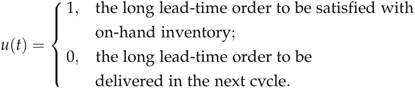
To maximize the profit in this inventory system with alternative lead‐time options, it is necessary for the supplier to find an optimal dynamic inventory‐commitment policy u(t) with respect to n(t), m(t), and the elapsed subperiod t. With an optimal inventory‐commitment policy, it is possible for us to address the issue of optimal inventory stocking, that is, to characterize an optimal inventory‐replenishment policy.
3. Optimal Inventory Commitment and Replenishment Policies
In this section, we study the problem of inventory management with alternative lead times in detail. We first develop an optimal inventory‐commitment policy in Subsection 3.1, and then characterize an optimal inventory‐replenishment policy in Subsection 3.2. Finally, we study an extended model that incorporates a supply‐capacity constraint in Subsection 3.3.
3.1. Optimal Inventory‐Commitment Policy
As the price for the short lead‐time customer ps is no less than the price for the long lead‐time customer pf , it is always beneficial for the supplier to satisfy the short lead‐time order as long as the on‐hand inventory is non‐zero. However, it is critical to decide when to fulfill orders from long lead‐time customers. In this section, we derive an optimal inventory‐commitment policy.
Let V(t, n, m) be the value function for subperiod t, with the on‐hand inventory and the promised‐for‐delivery products as n(t) and m(t), respectively. When n(t)=0, neither long lead‐time nor short lead‐time customers can be satisfied in the current cycle. Therefore, the demand from short lead‐time customers is lost, and orders for long lead‐time customers are scheduled to be delivered in the next cycle. The supplier obtains a revenue of pf
from each long lead‐time customer, that is, for 1≤t<T, 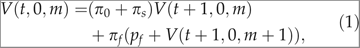
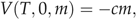

For n(t)≥1, with an admission control, the supplier decides when a long lead‐time customer should be satisfied. The dynamic programming equation for 1≤t<T is 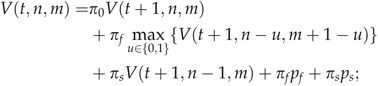

Equation (4) indicates that it is necessary to compare the profit between two possible actions: to use a unit of on‐hand inventory to satisfy the long lead‐time customer immediately, or to promise to deliver in the next cycle. The following lemma provides a monotonicity property of the profit difference between these two actions. Its proof appears in Appendix.
L
For a given m, For a given n,
 is nondecreasing in n; that is,
 .
. is independent of m; that is,
 .
.
Part (a) of the above lemma indicates that the greater the on‐hand inventory n is, the better it is for the supplier to use a unit of on‐hand inventory to satisfy the long lead‐time customer. More interestingly, part (b) of the above lemma reveals that this decision is independent of the promised‐for‐delivery level m. This is because the supplier takes care of the tradeoff between inventory‐holding cost for one unit product and possible profit from selling it to a short lead‐time customer. As revenue from a long lead‐time customer will not change even if the supplier delivers the product immediately, the promised‐for‐delivery level does not play in the tradeoff.
We now present a theorem that characterizes the optimal dynamic inventory‐commitment policy. Its proof is similar to that of Lemma 3.1. By using (4), we can obtain the desired results by checking the different cases of the term  in (4). We provide the proof in Appendix S1.
T
The optimal inventory‐commitment policy is characterized by a switching commitment level C
L
(t). The commitment level C
L
(t) equals 0 if
In each subperiod, the optimal control is to use a unit of the on‐hand inventory to satisfy orders from long lead‐time customers immediately if n(t)>CL(t); otherwise, to promise to deliver orders from long lead‐time customers in the next cycle.
 ; otherwise, it is defined as the maximum value of n such that
 . Moreover, the commitment level is independent of the promised‐for‐delivery level m, and has a continuity property with respect to the subperiod index t, that is,
 .
.
This theorem characterizes the optimal inventory‐commitment policy when the supplier encounters orders from long lead‐time customers. With such a commitment policy, the supplier balances the trade‐off between using on‐hand inventory and using replenished inventory in the next cycle. The former reduces the inventory‐holding cost; the latter keeps on‐hand inventory to meet potential short lead‐time orders in the rest of the cycle. Further, the inventory‐commitment levels are time dependent. This is because the supplier takes care of the tradeoff between inventory‐holding cost for one unit product and possible profit from selling it to a short lead‐time customer. As subperiod t advances, the remaining time of the cycle decreases, which leads to a smaller possibility for the supplier to sell it to a short lead‐time customer. Hence, the supplier is more likely to use its on‐hand inventory for long lead‐time customers to avoid the inventory‐holding cost, and therefore has a lower commitment level as time elapses.
R
3.2. Optimal Inventory‐Replenishment Policy
In the last subsection, we obtained the optimal inventory‐commitment policy for the supplier in a selling cycle. In this subsection, we extend our study to investigate the existence and form of the optimal inventory‐replenishment policy. We start with a single‐cycle problem.
Let  be the set of functions on
  , where N stands for {0,1,2, …}, and if
  , then:
 is nondecreasing in m for a given n; and
  is nondecreasing in n for a given m.
The following lemma claims that  . Again, the proof of the lemma appears in Appendix S1.
L , that is, V(t, n, m) satisfies P1, P2, and P3.
Note that the supermodularity of V(t, n, m) with respect to (n, m) means that the on‐hand inventory level and the amount of promised‐for‐delivery products are economic complements. At the beginning of the selling season, the supplier has an initial inventory n(0). A desired on‐hand inventory level is selected as n(1) s.t. n(1)≥n(0) to maximize profits, that is, 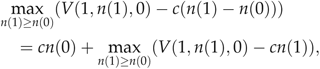
 is the purchasing cost. This can be easily solved because
  satisfies the property of P1. This result makes it possible for a further characterization of the inventory‐replenishment policy.
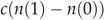
T such that the optimal ordering quantity is
 is the maximizer of
 , and it is independent of the initial inventory n(0).
3.3. Model with a Supply‐Capacity Constraint
In this subsection, we extend our basic model with a supply‐capacity constraint. The capacity constraint can be the outcome of the lead‐time requirement for replenishing inventory. Specifically, we assume that a replenishment order has one unit lead‐time, that is, the order Q of a cycle becomes available in the next cycle. Therefore, the inventory position n(t)+Q represents the maximum capacity for the rest of the current and the next cycles.
Compared with the basic model presented in Section 3.1, the orders from long lead‐time customers cannot be freely backlogged and satisfied in the next cycle. In this extended model, we include the following features: (1) unsatisfied long lead‐time orders are subjected to a penalty cost, and (2) the inventory‐commitment policy also considers possibilities for rejecting short and long lead‐time orders.
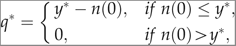
Denote Q and cp
as the size of the replenished inventory and the penalty cost for each unfulfilled long lead‐time order, respectively. Then, the value function  for subperiod
  is
is 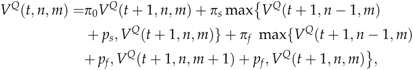
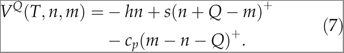
The value function (6) suggests that when a long lead‐time customer arrives, the supplier chooses the best action among three possible actions: to use a unit of the on‐hand inventory to satisfy the customer immediately, to promise to deliver the order in the next cycle, or to reject the order. When a short lead‐time customer arrives, the supplier chooses to use a unit of the on‐hand inventory to satisfy the customer immediately, or to reject the order. The following lemma provides the monotonicity properties of the value function. Again, the proof of the following lemma appears in Appendix S1.
L
For a given m,
For a given m,
For a given m,
 is nondecreasing in n; and for a given n,
 is nondecreasing in m.
 is nondecreasing in n (concavity in n); and for a given n,
 is nonincreasing in m (supermodular).
 is nondecreasing in n (supermodular); and for a given n,
 is nonincreasing in m (concavity in m).
Similar to results we developed for the basic model, the supermodularity of V(t, n, m) still holds with respect to (n, m) for the model with the supply‐capacity constraint. It reveals that the on‐hand inventory level and the amount of promised‐for‐delivery products are economic complements. To characterize the optimal inventory‐commitment policy for long lead‐time customers, we present the following definitions.
D
For each m, a commitment level C
L1(t, m) equals 0 if For each m, a commitment level C
L2(t, m) equals 0 if For each m, a commitment level C
L3(t, m) equals 0 if For each m, a commitment level C
L4(t, m) equals 0 if
 ; otherwise, the commitment level is defined as the maximum value of n such that
  .
. ; otherwise, the commitment level is defined as the maximum value of n such that
  .
. ; otherwise, the commitment level is defined as the maximum value of n such that
  .
. ; otherwise, the commitment level is defined as the maximum value of n such that
  .
.
Based on the above lemma and definitions, it is possible for us to present the following theorem that characterizes the optimal inventory‐commitment policy for both long and short lead‐time customers. This inventory‐commitment policy provides an optimal decision with respect to the state variables n and m. Its proof appears in Appendix.
T
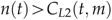
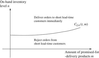
For subperiod t, for long lead‐time customers, the optimal inventory‐commitment policy is characterized by three switching commitment levels CL1(t, m), CL2(t, m), and CL3(t, m); and for short lead‐time customers, the optimal inventory‐commitment policy is characterized by CL4(t, m). The commitment level CL1(t, m) is nonincreasing in m, and commitment levels CL2(t, m), CL3(t, m), and CL4(t, m) are nondecreasing in m. When
When
The optimal inventory‐commitment policy for short lead‐time customers is to satisfy orders immediately if
 . That is, if
 , then
  .
. , the optimal inventory‐commitment policy for long lead‐time customers is to satisfy orders immediately if
 , to promise to deliver orders in the next cycle if
 , and to reject orders otherwise.
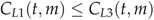 , the optimal inventory‐commitment policy for long lead‐time customers is to satisfy orders immediately if
 , and to reject orders otherwise.
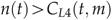 , and to reject orders otherwise.
This theorem provides the optimal inventory‐commitment policy for models with a supply‐capacity constraint. With the inventory‐commitment policy, the supplier balances the tradeoff between delivering products to satisfy customers immediately and to reduce on‐hand inventory, delaying the delivery of orders to the next cycle in anticipation of potential short lead‐time customer orders, and rejecting the long lead‐time orders to avoid the penalty costs in the case of failing to satisfy promised orders.
Inventory‐commitment policies for short and long lead‐time customers are illustrated in Figures 1 and 2, respectively. For short lead‐time customers, if the on‐hand inventory level and the promised‐for‐delivery level are high and low, respectively, it is rational to deplete the on‐hand inventory, and there is a low risk of running out of the capacity for promised‐for‐delivery products. Then, the optimal action is to use a unit of the on‐hand inventory. On the other hand, if the on‐hand inventory level and the promised‐for‐delivery level are low and high, respectively, then the supplier has insufficient on‐hand inventory and runs out of future capacity for the next replenishment. In this case, the optimal action is to reject the short lead‐time order.
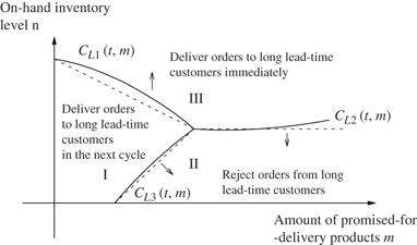
For long lead‐time customers, if both the promised‐for‐delivery level and the on‐hand inventory level are low, as illustrated by region I in Figure 2, the optimal action is to promise to deliver the order in the next cycle. If the promised‐for‐delivery level and the on‐hand inventory level are high and low, as they are illustrated by region II in Figure 2, the supply‐capacity constraint limits the potential delivery capacity. The optimal action is thus to reject the order. If the on‐hand inventory level is high, as illustrated by region III in Figure 2, the optimal action is to use a unit of the on‐hand inventory.
In addition, from (c) of the theorem, we know that the three switching commitment curves intersect at one point, because at each switching commitment curve, there are two actions leading to the same profit, and the supplier has three possible actions. This observation is not only interesting, but also has potential in constructing simplified control policies. With this observation, we can construct an approximation for the control region, as shown by the dotted line in Figure 2. To obtain this approximated control, we only need to find three points, the intersections of horizontal and vertical axes, and the intersection of the three curves. Note that the intersections of horizontal and vertical axes can be calculated by searching n, which makes the two terms 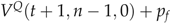 and
and 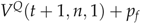 equal, and by searching m, which makes the two terms
 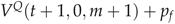 and
and  equal, respectively. The intersection of the three curves can be calculated by searching the (n, m), which makes the three terms
  and
and  equal.
T is nonincreasing in Q. (b)
  is nondecreasing in Q. (c)
  is nondecreasing in Q. (d) When Q increases, CL1(t, m) moves right‐upward in
Figure 2, and CL2(t, m) and CL3(t, m) move right‐downward in
Figure 2
.
is nondecreasing in Q. (d) When Q increases, CL1(t, m) moves right‐upward in
Figure 2, and CL2(t, m) and CL3(t, m) move right‐downward in
Figure 2
.
This theorem reveals the relationship between the optimal inventory‐commitment policy and the supply capacity Q. Its proof appears in Appendix. When the supply capacity increases, it is more likely that the supplier satisfies orders immediately or promises to deliver orders to the next cycle. As Figure 2 shows, rejection‐region II diminishes and promised‐for‐delivery region I expands. When Q goes to infinity, it is reduced to the basic model studied in Theorem 3.1, and rejection‐region II disappears.
R , which means that one more unit of penalty cost is incurred whenever the supplier accepts either a short or a long lead‐time customer. In this case, we have three cases. When ps
+h<cp
, all of the short and long lead‐time customers are rejected. When pf
+h>cp
, all of the short and long lead‐time customers are accepted. When pf
+h<cp
<ps
+h, all of the short lead‐time customers are rejected and all the long lead‐time customers are accepted. By backward induction, these results can be obtained from dynamic programming Equations (6) and (7).
, which means that one more unit of penalty cost is incurred whenever the supplier accepts either a short or a long lead‐time customer. In this case, we have three cases. When ps
+h<cp
, all of the short and long lead‐time customers are rejected. When pf
+h>cp
, all of the short and long lead‐time customers are accepted. When pf
+h<cp
<ps
+h, all of the short lead‐time customers are rejected and all the long lead‐time customers are accepted. By backward induction, these results can be obtained from dynamic programming Equations (6) and (7).
4. Study of the Inventory‐Rationing and Inventory‐Commitment Policies
In Theorem 3.1, we prove that the optimal inventory‐commitment policy depends on a time‐dependent switching commitment level for long lead‐time customers. In the inventory‐rationing literature, for each demand class, a class of inventory‐rationing policy is to choose a static value that defines the maximum number of orders to be reserved for the corresponding class. Cattani and Souza (2002) compare the performance of such an inventory‐rationing policy with the performance of a first‐come first‐served policy. They conclude that the former outperforms the latter. In contrast to the inventory‐rationing policy, the inventory‐commitment policy accepts orders dynamically. In this section, we carry out a study to compare the performance of the inventory‐commitment policy with that of the inventory‐rationing policy.
According to Theorem 3.1, the inventory‐commitment policy is defined by an optimal commitment level CL (t) for each t. The commitment level varies with respect to t (see Figure 3 for illustration). The supplier commits one unit of the on‐hand inventory to a long lead‐time customer as long as the on‐hand inventory level is higher than the commitment level. The inventory‐rationing policy, in contrast, depends on one static inventory‐rationing level. With the prevailing probabilities of the demand classes listed in Table 1, we calculate the profits under the dynamic and static policies. Note that the optimal inventory‐rationing level is obtained by a complete enumeration. Assume that pl =αps and α≤1. We use α as the price‐decline rate. Let ps =100, c=70, and the salvage value s=20. In this section, we use the single‐cycle model to carry out numerical experiments for different values of inventory‐holding cost h and price‐decline rate α.
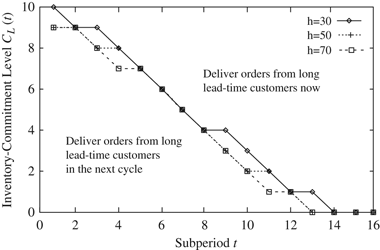
Let α=0.95, and we calculate the optimal inventory‐commitment levels in Figure 3, which are nonincreasing with respect to the subperiod index. We obtain the optimal profit with respect to different inventory‐holding costs in Table 2. The inventory‐rationing policy is implemented by enumerating the rationing levels. The improvement ratio is defined as the profit difference between two policies divided by the profit of the inventory‐rationing policy. Then, we let h=50, change α, and obtain the corresponding optimal profit and improvement ratio in Table 3. From Tables 2 and 3 we see that the optimal profit for the inventory‐commitment policy is greater than that of the inventory‐rationing policy, and the improvement ratio is greater than 4%.
Further, we reduce the horizon length to 8 and obtain the profits for the inventory‐commitment and inventory‐rationing policies as 193.91 and 190.24, respectively. The improvement ratio is 1.9%, which is smaller than the improvement ratio for the model in which the horizon length is 16. This observation is intuitively true. As discussed after Theorem 3.1, we indicate that the inventory‐commitment levels are time dependent. A smaller t leads to a greater commitment level. Hence, the inventory‐commitment levels vary in a longer horizon. This demonstrates that the benefit of deploying the inventory‐commitment policy increases as the length of the cycle increases.
4.1. Robustness of the Inventory‐Commitment Policy
From Figure 3, the trajectory of the optimal inventory‐commitment policy seems to suggest that the optimal commitment levels are not sensitive with respect to inventory‐holding cost h. This implies that the inventory‐commitment policy can be deployed even when the value of the inventory‐holding cost is uncertain or difficult to obtain. Now, we carry out a numerical experiment to verify this observation. This experiment enables us to quantify the performance changes when an estimated inventory‐holding cost parameter is used to derive the inventory‐commitment policy. Table 2 shows that when the inventory‐holding cost h=60, the optimal profits for the inventory‐rationing and inventory‐commitment policies are 308.09 and 321.12, respectively. Now, we assume that the inventory‐holding cost for the problem under investigation is h=60. Instead, the supplier uses the dynamic inventory‐commitment policies derived for h=70 and 50, and the corresponding profits are 320.65 and 321.10, respectively. Therefore, a 1/6 change in the inventory‐holding cost yields less than 0.15% change in profit. In addition, the dominance over the performance of inventory rationing is maintained. We believe that this observation results from the fact that the inventory‐commitment policy dynamically changes the on‐hand inventory over the entire cycle and that the end inventory is consistently lower. As the inventory‐holding cost applies only to the ending inventory, it is rational to expect such performance.
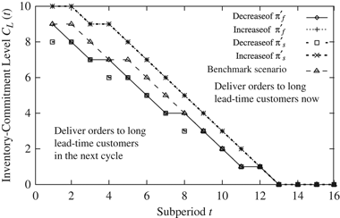
Further, we change the demand rates in the subperiods. We use the demand rates represented by short, long lead‐time demand, and no demand probabilities π′
s, π′
f
, and π′0 in Table 1 as the benchmark probabilities. First, we fix π′
s
, and let π′
f
have a decrease (increase) of  (
( ). We then fix π′
f
, and let π′
s
have a decrease (increase) of
). We then fix π′
f
, and let π′
s
have a decrease (increase) of  (
( ). Let α=0.95 and h=70. Then, we compare the inventory‐commitment levels for the decrease/increase of the long lead‐time demand model, the decrease/increase of the short lead‐time demand model, and the benchmark case presented in Figure 4. The profits for these models are listed in Table 4, in which the change rate is equal to the difference between the profit for the corresponding model and the optimal profit divided by the optimal profit. The results demonstrate that the degree of profit change is marginal. We believe that the downward slope of the commitment level with respect to time makes the difference here.
5. Benefit of the Choice Model: Demand‐Induction and Demand‐Cannibalization Effects
By deploying the inventory‐commitment policy, we find that the supplier pools the uncertainties of short and long lead‐time customers together. This risk‐pooling effect seems to suggest that it is quite promising for a supplier to introduce alternative lead times. However, at the same time, we have to note that customers could change their ordering patterns in anticipation of an alternative lead time. Therefore, in this section, to further evaluate the benefits and drawbacks of providing an alternative lead time to customers, we consider the demand‐induction and demand‐cannibalization effects with non‐choice and choice models (Gallego and Phillips 2004, Novshek and Sonnenschein 1979).
5.1. Analytical Results for Non‐Choice and Choice Models
In this subsection, we first characterize the non‐choice model. Then we develop the choice model and analyze the probabilities changes for these two models. Specifically, we assume the customer's maximum willingness to pay (WTP) for products with current and next‐cycle deliveries is ws
and wl
, respectively, where ws
and wl
depend on a joint distribution over  of
of  .
.  is a set of two‐dimensional non‐negative vectors.
In a non‐choice model,
1
the supplier provides products with a short lead‐time delivery only. Then, the customer buys products as long as its WTP is no less than the price of the product with a short delivery lead time, that is, ws
≥ps
. Then, the probability of the prevailing short lead‐time customers is 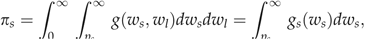
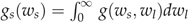 . If ws
and wl
are independently and uniformly distributed in [0, Ws
] and [0, Wl
], respectively, then we can obtain that
. If ws
and wl
are independently and uniformly distributed in [0, Ws
] and [0, Wl
], respectively, then we can obtain that 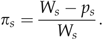
The probability of no show is π 0=1−πs . In this model, all short lead‐time customers are satisfied once the supplier has non‐zero on‐hand inventory.
In the choice model, the supplier provides two alternative delivery lead times. In this case, probabilities are different for these customers, which is due to demand‐induction and demand‐cannibalization effects. In what follows, we develop models for the demand induction and cannibalization. Before that, we need some notations.
We assume that the maximum WTP for the long lead‐time delivery mode wf
is a linear function of the current and the next‐cycle delivery WTP, 
Demand induction is defined as the extra long lead‐time demand that is induced by the possibility of obtaining the desired product right away. These customers would not exist without the alternative lead‐time option. It is assumed that the price of the long lead‐time product is no more than that of the short lead‐time product, that is, pf
≤ps
. The demand induction takes place when the WTP of a short lead‐time customer is lower than the prevailing short lead‐time price ps
, and the WTP of a long lead‐time customer is higher than the prevailing long lead‐time price pf
, that is, 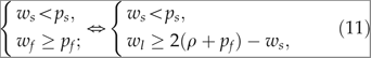
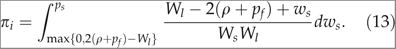
 ” is by (10). Then, we determine that the probability of the induced demand is
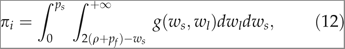
Demand cannibalization is defined as the short lead‐time demand that is induced by the possibility of obtaining the desired product immediately by presenting it as a long lead‐time request. These customers would not be entertained without the alternative lead‐time option. Note that for the specific prices of the two lead‐time choices, customers are defined as the short lead‐time type when they choose the short lead‐time option, and the choices of these customers change when prices change. For example, when the price of the alternative long lead‐time choice is modified to be low enough to compensate some customers for the penalty of dissatisfaction in the current cycle, these short lead‐time customers switch to the long lead‐time option. Thus, they become long lead‐time customers when prices are lowered. Demand cannibalization takes place when the WTP of a short lead‐time customer is higher than the prevailing short lead‐time price ps
, and the margin (the WTP wf
minus the price pf
) of the long lead‐time option is greater than the margin of the short lead‐time option, that is, 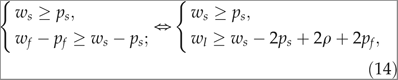
 ” is by (10). Then, we obtain that the probability of the cannibalized demand of the choice model is
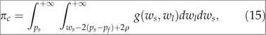
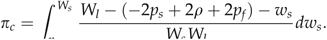
From the above equations, we know that the cannibalized demand πc decreases in the prevailing long lead‐time price pf .
According to the foregoing analysis, the probabilities can differ for the choice model. The probability of the prospective short lead‐time customers is reduced by the demand‐cannibalization effect πc , and the probability of the prospective long lead‐time customers is equal to the sum of the cannibalized and the induced demands. Therefore, π′0 of the Choice Model=π 0 of the Non‐choice Model –πi ; π′ s of the Choice Model=πs of the Non‐choice Model –πc ; and π′ f of the Choice Model=πi +πc . With (12) and (15), it is possible for us to calculate the probabilities for each subperiod. In the next subsection, we present results from a numerical study.
5.2. Numerical Results
To study the demand induction and cannibalization effects via numerical experiments, we do not need to select several values for the penalty ρ, because it is constant for customers, and, by (13) and (16), it can be considered together with the price for long lead‐time option pf
. We assume that ρ=3, ps
=100, pf
=95, and Wl
=Ws
. We set  and the value of Ws
and the prospective probabilities are listed in Table 5. π
0=1−πs
. By (13) and (16), we calculate the probabilities for each subperiod in Table 1.
and the value of Ws
and the prospective probabilities are listed in Table 5. π
0=1−πs
. By (13) and (16), we calculate the probabilities for each subperiod in Table 1.
Then, we use (4) and (5) to calculate the profit for the non‐choice (π
0 and πs
are in Table 5, and πf
=0) and choice models (π′0, π′
s
, and π′
f
are in Table 1), and compare the profit of these two models. We obtain that the optimal profit increases by  when a long lead‐time choice is provided, even with the price decline of the long lead‐time product.
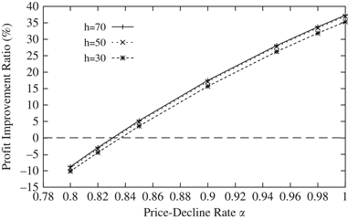
In addition, we compare the maximal profits between the non‐choice and choice models with different price‐decline rates α, defined as pf /ps and inventory‐holding cost h. The results are illustrated in Figure 5, in which the profit improvement ratio is defined as the profit difference between the non‐choice and choice model divided by the profit of the non‐choice model. We can see that the profit improvement for introducing a lead‐time option can be significant, and the greater the price‐decline rate (the larger the inventory‐holding cost), the greater the improvement ratio. The improved profit comes from (1) the demand induction, that is, the lower price of long lead‐time products attracts additional customers; and (2) the risk‐pooling effects, that is, long lead‐time customers provide flexibility to the supplier regarding the delivery time of the products. However, when the price decline is significant, introducing a long lead‐time option may have a negative impact, with demand cannibalization, whereby, some short lead‐time customers switch to being long lead‐time customers. In addition, the profit improvement is not sensitive to the inventory‐holding cost. This observation suggests that the leftover inventory level for non‐choice and choice models are comparable, because the choice model not only pools the uncertainties of short and long lead‐time customers, which reduces the leftover inventory level, but it also starts with a higher inventory level, which increases the leftover inventory level.
6. Concluding Remarks and Directions for Future Research
This paper introduces lead‐time choices for customers to the traditional fixed and unique lead‐time inventory model. Customers are modeled to be in two categories: those with a short and a long lead‐time requirement. The former asks for a delivery lead time that is within the current production cycle of the supplier, and the latter asks for a delivery lead time that can be within the current production cycle, or in the next production cycle.
For this basic inventory model without supply‐capacity constraint, in which a supplier provides short and long lead‐time alternatives to its customers, we characterize an optimal inventory‐commitment policy, that is, whether to use a unit of the on‐hand inventory to satisfy a long lead‐time customer. Further, we prove that the optimal inventory‐replenishment policy is a base‐stock type.
With the above results, we extend our model to accommodate a supply‐capacity constraint. With the constraint, the optimal inventory commitment for short lead‐time customers is characterized by a switching commitment level. Based on the relations of the on‐hand inventory and this switching commitment level, the optimal inventory‐commitment policy controls the admission of short lead‐time customers. The optimal inventory commitment for long lead‐time customers is characterized by three switching commitment levels. These levels, based on the on‐hand inventory and promised‐for‐delivery, determine when to accept, backlog, or reject long lead‐time customers.
With both the analytical results and numerical experiments, this paper demonstrates that offering alternative lead‐time choices can improve the supplier's profit. The improved profit comes from the following sources. (1) The demand‐induction effect: the lower price of the long lead‐time choice attracts additional customers. (2) The risk‐pooling effects: the long lead‐time customers provide flexibility to the supplier regarding the delivery time of the products. The supplier balances the trade‐off between (a) promising to deliver products in the next cycle to save on‐hand inventory, which meets potential short lead‐time orders in the remaining cycle; or (b) using a unit of the on‐hand inventory immediately to satisfy long lead‐time customers to reduce the inventory‐holding cost. This enables the supplier to use the future capacity together with the current capacity to satisfy demands from different customer classes. This also enables the supplier to better control the on‐hand inventory during a selling cycle. However, when the price decline of the long lead‐time option is significant, introducing lead‐time choices can also have a negative impact.
Note that the risk‐pooling, demand‐induction, and demand‐cannibalization effects of flexible products in a revenue management model are investigated by Gallego and Phillips (2004) and Gallego et al. (2006). The concept of flexible products is similar to that of long lead‐time products, because both let the supplier choose from a feasible set, such as, two feasible products or two feasible delivery lead times. However, the concept of long lead‐time products that is presented in this paper focuses on the flexibility of delivery time rather than on the flexibility of what is being delivered. For the single‐cycle setting, we deal with an optimal control problem that has dynamic programming equations that are similar to those in Gallego et al. (2006) but with different boundary conditions, and derive the optimal inventory‐replenishment policy at the beginning of the cycle. We also extend the obtained results to a multi‐cycle setting, and obtain the optimal inventory‐replenishment policy and the inventory‐commitment policy for multi‐cycle problems.
In addition, this paper compares the profits of the supplier under the optimal inventory‐commitment policy and the inventory‐rationing policy. Cattani and Souza (2002) compare the inventory‐rationing policy with the first‐come first‐served policy and evaluate the conditions under which the inventory‐rationing policy is beneficial. This paper demonstrates that the optimal inventory‐commitment policy outperforms the inventory‐rationing policy, especially when the inventory‐holding cost is low and the cycle time is long. In addition, the optimal commitment level in each subperiod is robust to the inventory‐holding cost and the probabilities in subperiods, so that the supplier can achieve a close‐to‐optimal profit even when these parameters are not fully estimated.
We consider scenarios for extending our model. One extension is to consider a multi‐cycle incapacitated model, in which, the leftover products are carried over to the subsequent cycle. Then, at the beginning of each cycle (except for the first cycle), the inventory‐replenishment function acts: (1) to satisfy the orders that were promised in the previous cycle; and (2) to build up inventory for future orders. Without a supply‐capacity constraint, these two functions can be carried out separately, as orders that were promised in the previous cycle are known when the replenishment decision is made. The third extension is to incorporate another penalty cost cps for rejecting a short lead‐time customer into the capacitated model. We can demonstrate that our analysis of the basic model can be carried out for these three extensions, that is, the inventory‐commitment and the inventory‐stocking policies remain optimal. The details are omitted here due to space limitations.
A fourth interesting extension is to consider the risk of customer order cancellations. In this case, the cancellation model, a customer may cancel the order (e.g., due to changes in economic conditions). We prove that a similar inventory‐commitment policy is optimal. However, the new inventory commitment level for the cancellation model is nonincreasing in the promised‐for‐delivery level m, rather than independent of m as in Theorem 3.1. The larger m is, the greater the number of possible canceled orders is. This, in turn, results in a larger possible leftover inventory and encourages the supplier to use its on‐hand inventory to satisfy long lead‐time customers. In other words, the risk of order cancellations makes a supplier more likely to use on‐hand inventory for long lead‐time customers. A detailed model and its proof can be found in the online Appendix S1.
In this paper, we have assumed that the prices for both short and long lead‐time customers are exogenously decided. It would be interesting to extend this model with pricing features. However, we believe that the existence of both demand‐induction and demand‐cannibalization effects could complicate the analysis. Therefore, simple models that isolate either the demand‐induction or the demand‐cannibalization effect may assist the analysis. Another interesting area for further study would be to extend this work to deal with a positive replenishment lead time L, L≥1. With this feature, it would be possible for the supplier to provide multiple lead‐time options to customers.
Footnotes
Appendices
1Note that the analysis in this section focuses on the model without a capacity constraint. When we incorporate the capacity constraint into these non‐choice and choice models, it complicates the problem. See online Appendix S1 for details.
Acknowledgments
The authors are grateful to the senior editor and the three anonymous reviewers for their detailed and valuable suggestions and comments.