
Abstract
Resource flexibility is an important tool for firms to better match capacity with demand so as to increase revenues and improve service levels. However, in service contexts that require dynamically deciding whether to accept incoming jobs and what resource to assign to each accepted job, harnessing the benefits of flexibility requires using effective methods for making these operational decisions. Motivated by the resource deployment decisions facing a professional service firm in the workplace training industry, we address the dynamic job acceptance and resource assignment problem for systems with general resource flexibility structure, i.e., with multiple resource types that can each perform different overlapping subsets of job types. We first show that, for systems containing specialized resources for individual job types and a versatile resource type that can perform all job types, the exact policy uses a threshold rule. With more general flexibility structures, since the associated stochastic dynamic program is intractable, we develop and test three optimization‐based approximate policies. Our extensive computational tests show that one of the methods, which we call the Bottleneck Capacity Reservation policy, is remarkably effective in generating near‐optimal solutions over a wide range of problem scenarios. We also consider a model variant that requires dynamic job acceptance decisions but permits deferring resource assignment decisions until the end of the horizon. For this model, we discuss an adaptation of our approximate policy, establish the effectiveness of this policy, and assess the value of postponing assignment decisions.
Keywords
1. Introduction
Resource flexibility, the ability of manufacturing or service resources to perform many different job types, is an important tool for firms to cope with the uncertainties in the mix and volume of demand. For given total capacity, higher flexibility permits meeting more of the demand by adjusting the deployment of the flexible resources. This ability to match demand with available capacity is critical in today's highly competitive and dynamic environment in which firms must offer a wide variety of products and services while simultaneously ensuring high service levels and good resource utilization. The operations management literature on flexibility largely emphasizes strategic issues and insights such as the role of flexibility in handling uncertainties and the level of flexibility needed to maximize expected profits or minimize lost sales. These models simplify the operational issues of how much of each product's demand to serve and how to deploy the available resources by assuming that these decisions are made only after observing all demand. In service settings, however, demand acceptance and resource assignment decisions must be made as demand arises, without complete information; hence, harnessing the benefits of flexibility requires effective operational policies. As Maister (1997) notes, service firms often treat these decisions as routine scheduling functions and tend to underestimate their impact; however, they are critical to firm profitability since the dynamic resource deployment decisions largely govern revenue generation and resource utilization. This paper is motivated by the dynamic demand selection and resource assignment decisions facing a workplace training firm that uses instructors with varying levels of expertise to offer different types of training programs. The goal of this research is to develop effective methods to support deployment decisions for flexible resources in such settings.
The workplace training industry has grown significantly in recent years, driven by the competitive imperative for firms to continuously upgrade the knowledge and skills of their employees in order to cope with the rapid technological changes and business trends such as outsourcing and globalization of markets and competition. According to the 2007 State of the Industry Report by the American Society for Training and Development, training expenditures of large organizations increased from 1.8% of total annual payroll costs in 1997 to 2.33% in 2006, with an average annual training expenditure of over $1,000 per employee (Paradise 2007). Outsourced training accounts for around 28% of total training expenditures, with face‐to‐face delivery continuing as the dominant (over 70%) form of training. These pressing corporate training needs have led to the emergence of several workplace training companies that provide on‐site training for client corporations by offering short‐term educational programs on various topics such as leadership, quality, negotiation, and global management. To offer these different programs, training firms employ instructors with varying capabilities—some instructors are qualified to teach only one particular type of training program, whereas others are experienced enough to teach multiple types of programs. At the strategic level, the training firm must decide what types of training programs to offer, how to price these programs, and how many flexible and specialized instructors to employ. Given these choices, we study how the firm should dynamically respond to incoming requests for training on a particular date in order to maximize expected profits. Soon after receiving a client program request for this date, the firm must first decide whether to accept or decline this job; if accepted, the firm must also decide which among the available and qualified instructors or resources to assign to the job. These job acceptance and resource assignment decisions, constituting the dynamic resource deployment problem, must incorporate the following core tradeoff. By accepting the current request, the firm foregoes the opportunity to use the resource for a more profitable future request. On the other hand, if the firm declines the current request, it faces the risk of having to later assign the resource to a less profitable program or leaving the resource idle on the training date. With flexible resources, the problem is even more challenging due to the complex interrelationships between the acceptance and assignment decisions across job and resource types. The optimal decision depends on factors such as the number and flexibility of available resources, relative profitability of different job types, and the volume, mix, and variability of future demand.
Past research on flexibility has focused primarily on long‐term capacity planning and optimal investment strategies for flexible resources. Fine and Freund (1990), Jordan and Graves (1995), Van Mieghem (1998), Netessine et al. (2002), Bish and Wang (2004), and others study the value of flexibility as a hedge against uncertainty. Using stylized models, they develop insights or methods to determine the optimal level of investment in flexible and specialized capacities for manufacturing firms that face uncertainty in the volume and mix of demand. Typically, these models represent the capacity planning problem as a profit maximizing two‐stage stochastic program in which the first stage selects the capacity levels and the second stage allocates the realized demand to the available capacity. Since these models focus on the higher‐level capacity planning decisions, they assess the value of each candidate capacity portfolio by assuming that, at the second stage, the firm can optimally select the demand to serve and the resources to assign after observing all of the demand. For service operations contexts in which job acceptance and resource assignment decisions must be made soon after each job arrives, this “perfect demand information” assumption overestimates the true profit impact of capacity choices. Our work seeks to develop methods for dynamic resource deployment without full knowledge of demand, but assuming given capacity and flexibility levels.
Like the problem we study, revenue management (e.g., Talluri and Van Ryzin 2004) also deals with dynamic decisions on using resources whose output cannot be inventoried. However, our flexible resource deployment problem differs in two important ways from traditional revenue management applications in service industries such as airlines, hotels, and car rental agencies (e.g., Cross 1997, Dietrich et al. 2008, Geraghty and Johnson 1997, Sen and Zhang 1999, Smith et al. 1992). First, in these revenue management contexts, the resource structure is quite specialized, eliminating or simplifying the resource assignment decisions. For instance, many airline seat allocation models assume a single versatile resource type (e.g., economy class seats) that can accommodate all demand types (e.g., fare classes), and hence focus solely on demand acceptance decisions. Similarly, the stochastic knapsack problem (e.g., Kleywegt and Papastravou 1998, Ross 1996), applicable to production and transportation contexts, focuses on acceptance decisions for jobs (with varying sizes and revenues) using a single resource type. In other applications, resources have a hierarchical structure that permits full downward resource substitution (e.g., a premium car can be downgraded to satisfy a request for a standard or compact car). In contrast, the resource flexibility structure in training firms is much more complex. Resources are not identical nor do they have a complete ordering in terms of their flexibility because different resource types can have arbitrary overlaps in their service capabilities. Second, in some revenue management contexts, firms can regulate demand by changing prices dynamically, whereas pricing decisions for training services are strategic (e.g., based on competitive factors or long‐term client relationships) and therefore fixed during the operational decision horizon.
For call center management, another context that entails dynamic service decisions, researchers have studied skills‐based routing policies to assign inbound calls to multi‐skilled agents who can handle different call types (Aksin et al. 2007 and Gans, Koole, and Mandelbaum 2003 provide comprehensive surveys of call center models). However, call centers are also quite different from our problem context. First, incoming calls require service as soon as possible, and queue up until the next available agent is assigned to the call. The time to process each call is stochastic, and agents can handle multiple calls in sequence during each time interval. In contrast, for our problem setting, each accepted job requires service on the specified training date at the end of the horizon, and each resource can handle only one job. Second, most skills‐based routing models focus on resource assignment and do not simultaneously consider call admission, whereas our problem requires joint consideration of job acceptance and resource assignment decisions. Third, call center models focus on minimizing expected waiting time or customer abandonment rate, while our objective is to maximize the expected profit. Queuing models provide a natural representation of call centers, and stochastic dynamic programming is a standard approach for determining optimal routing policies in Markov queues. Because the state space is prohibitively large for practical problems, researchers have only studied optimal call‐routing policies for simplified systems with two call types and the following three canonical designs (Garnett and Mandelbaum 2001): V‐design systems consisting of a single pool of crossed‐trained agents (e.g., Armony and Maglaras 2004a, b, Bhulai and Koole 2003, Gans and Zhou 2002), N‐design systems containing two pools of resources, one dedicated to one of the job types and the other capable of handling both job types (e.g., Xu et al. 1992), and M‐design systems having two pools of specialized resources and a common pool of flexible agents (e.g., Ormeci 2004). For systems with more than two call types and more complex resource flexibility structures, researchers have proposed various heuristic methods, such as static priority policies (Shumsky 2004, Stanford and Grassman 2000) and schemes based on age factors for different call types (Perry and Nilsson 1992).
The process of booking training programs also differs from contexts such as airline reservations and call centers because it is a business‐to‐business interaction. For instance, clients seeking training programs are willing to wait a few days for a response, permitting the training firm to decide on pending requests periodically rather than responding instantaneously to each request. Further, the general resource flexibility structure necessitates simultaneous consideration of job acceptance and resource assignment decisions (to ensure that a set of accepted jobs is feasible, given the number and mix of available resources).
In section 2, we formulate the flexible resource deployment problem as a profit‐maximizing discrete‐time stochastic dynamic program, and discuss a deterministic model to generate upper bounds on the optimal profits. We focus on situations that require the firm to decide both job acceptance and resource assignments in each period, but later discuss a variant in which the resource assignment decisions can be deferred until the end of the decision horizon. For either case, since the state space is very large, finding the exact policy by solving the associated Bellman equations is impractical. Section 3 analyzes the special case of a system containing specialized resources for each job type and a versatile resource type that can perform all job types, with no more than one job arriving in each period. For this setting, we show that the exact policy uses a threshold rule and identify some principles underlying this policy. In section 4 we develop three approximate policies for job acceptance and resource assignment for general resource flexibility structures and job arrival processes. The first two policies, called Deterministic Capacity Allocation (DCA) and Nested Capacity Reservation (NCR), explicitly account for the resource flexibility structure and demand stochasticity, respectively, while the third approach, called Bottleneck Capacity Reservation (BCR), jointly considers both dimensions. Section 5 reports the results of our extensive computational tests to assess the effectiveness and robustness of these policies under various operating environments, such as different levels of resource availability and flexibility. We benchmark the performance of the approximate policies against both a first‐come first‐served (FCFS) approach and the exact policy or perfect‐information (PI) solution (which provides an upper bound on exact profit). Our computational results, for 25 different problem scenarios, with numerous replications for each, consistently confirm that our dynamic policies are very effective. For problem instances that we could also solve exactly, the profits from our best policy deviates from optimality by only 1.28% on average (and a maximum of 2.22%) compared with 18.79% for the FCFS policy. Section 6 discusses the model variant when acceptance decisions must be made in each period but resource assignments can be deferred until the end of the decision horizon. We present the modified problem formulation for this variant, demonstrate how to adapt one of our approximate policies, and report computational results both to demonstrate the effectiveness of this policy and to assess the value of deferring assignments. Section 7 concludes the paper.
2. Problem Definition and Formulation
Consider a firm that offers several different service types using resources with varying levels of flexibility. In the workplace training context, the service types correspond to different training programs that the firm offers, and the resources are instructors who can teach one or more of these programs. Client requests for training programs arrive randomly, each specifying the type of program needed and the date on which the program is to be offered. We focus on the demand acceptance and resource assignment decisions for program requests for a particular date in the future. We refer to requests for training on this service date as jobs; the decision horizon is the time interval during which clients can request training on this date. Every accepted job requires one resource with the appropriate capabilities, and a resource cannot be assigned to more than one job.
Typically, each client requesting a training program expects a prompt, but not necessarily immediate, response from the training firm on whether the firm is willing to conduct the program. Depending on the response times that clients expect, the training firm may be able to accumulate a few requests before deciding which programs to accept. Thus, unlike real‐time business‐to‐customer interactions such as airline reservation systems or call centers that may require real‐time policies, the process of booking training programs is a business‐to‐business interaction for which a discrete‐time framework is appropriate. 1 This framework has the advantage of providing some latitude for modeling different situations. For instance, by making the period length small enough so that no more than one request arrives in each period, we can model immediate acceptance decisions for each individual request, whereas increasing the period length permits us to assess the benefits of demand accumulation. We can also vary the period length within the decision horizon to represent, for instance, quicker response requirements as the program offering date approaches. Turning to the frequency and timing of the resource assignment decisions, workplace training often involves some customization of the training program to the client firm. Hence, client firms as well as instructors prefer to have as much lead time as possible before the program date in order to prepare for the engagement. In this situation, the training firm makes acceptance and assignment decisions concurrently, i.e., when the firm accepts a program request it also assigns a specific instructor to the job rather than deferring the assignment decisions until the end of the decision horizon. Accordingly, our initial model incorporates dynamic decisions for both job acceptance and resource assignment; in section 6, we address the model variant in which assignment decisions may be deferred until the end of the decision horizon. As we explain later, deferring the assignments does not reduce problem difficulty since making dynamic job acceptance decisions requires simultaneously developing a resource allocation plan, albeit tentative, to ensure that the acceptance decisions are feasible.
The firm's goal is to maximize the expected total net revenue over the decision horizon. In making the job acceptance and resource assignment decisions in each period, the firm must consider the probability distribution of future demand, the availability of instructors and their flexibility, and the profitability of different types of programs. We next introduce our notation and formulate the decision problem as a stochastic dynamic program.
2.1. Stochastic Dynamic Programming Formulation
Given the set of available resources and their capabilities, and the demand distribution and profit margin for each job type, the flexible resource deployment problem entails deciding which incoming jobs (service requests) to accept in each period before the service date and what resource to assign to each accepted job in order to maximize the total expected profit. We model this problem as a stochastic dynamic program in which stages correspond to periods of the finite decision horizon. Let
The definition of job and resource types, with the associated capability sets, permits modeling a wide variety of situations. For instance, if profit margins vary by customer class or if certain customers have specific resource preferences, we can capture these features by defining separate job types for such customers. Similarly, although price is not a decision variable, we can incorporate different pre‐determined price categories (analogous to fare classes in airline reservations) for the same service by introducing one job type corresponding to each price. We can also include additional costs (e.g., goodwill loss) for not accepting jobs. Specifically, if αj denotes the penalty cost for rejecting a type‐j job, we can account for this cost by redefining the parameter πj for type‐j jobs as the profit margin for this job type plus the penalty αj .
We consider dynamic decisions over a decision horizon consisting of T periods, indexed backwards from t=T to 1. Period T denotes the start of the decision horizon, and period 1 is the last period for customer requests before the service date. As noted earlier, the choice of period length, which can vary during the decision horizon, depends on the desired customer response lead time and determines the extent to which demands can be accumulated before making acceptance and assignment decisions. In the limit, by choosing very short period lengths, we can model situations in which the firm must make acceptance and assignment decisions as soon as each job arrives.
For r∈
The stochastic dynamic programming formulation of the flexible resource deployment problem consists of T stages, one for each period t=1, 2, …, T. The resource availability vector 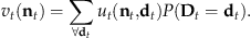
The profit‐to‐go ut
(
the demand constraints the resource availability constraints
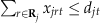 for all j∈
 for all r∈
Let  denote the action set containing all the feasible assignments for resources in period t, given the state (
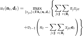
That is, the profit‐to‐go ut
(
Finding the exact policy, i.e., the profit‐maximizing dynamic policy for optimal job acceptance and resource assignment decisions at each period, is computationally intractable because the state space grows exponentially with the number of jobs, resources, and time periods. Next, we consider a deterministic version of the problem that provides upper bounds on the maximum expected profit for the stochastic problem and also underlies approximate policies.
2.2. Deterministic Acceptance and Resource Assignment Problem
Suppose, at period t, we know with certainty the cumulative future demand cdjt
of each job type j∈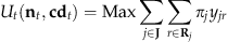
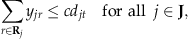
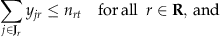

Given the solution 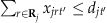 and resource allocations
 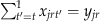 for all r∈
Since this model assumes that future demand is known, we refer to it as the Deterministic demand selection and resource assignment (DD) model. We can transform the optimization problem (3)–(6) into a single‐commodity minimum cost network flow problem defined over a network containing m job nodes, l resource nodes, and an additional source node. Since the minimum cost network flow model has an integer optimal solution if demands and capacities are integer‐valued, we do not need to explicitly impose integrality restrictions on the y‐variables.
The DD problem is easy to solve for certain special resource flexibility structures. Consider, for instance, a system containing m resource types, indexed as r=1, 2, …, m, with resource type r capable of performing job type j=r and all less profitable (higher‐indexed) job types, i.e., with
For the stochastic problem, the DD model, applied using appropriate point estimates of demand, may serve to guide resource allocation decisions for approximate policies. Moreover, as we discuss next, this model is also useful for generating upper bounds on the optimal value of the stochastic problem. First, suppose we solve this model for every possible realization 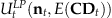 be the optimal value of its linear programming relaxation. The following proposition relates this value to the expected PI value E[Ut
(
be the optimal value of its linear programming relaxation. The following proposition relates this value to the expected PI value E[Ut
(
P .
.
P . Moreover, given the actual demand realization vector
 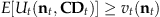 . □
. □
Proposition 1 states that the optimal value of the expected demand model is an upper bound on the expected PI value which in turn overestimates the expected profit of the exact dynamic policy. Since finding the exact policy is intractable, Proposition 1 provides a means to assess the effectiveness of approximate policies by comparing their expected profits to either of these upper bounds. Bertsimas and Popescu (2003) developed similar bounds for a network revenue management problem. Next, we analyze the structure of the exact dynamic policy for a special case, and later (in section 4) develop approximate policies for the general problem.
3. Analysis of Exact Policy with Specialized and Versatile Resources
Consider a system containing m specialized resource types, one for each job type, plus a versatile resource type that can perform all job types. We refer to this configuration of resource capabilities as the Star flexibility structure; it generalizes the M‐design structure (for two job types) that researchers have previously studied in other contexts (e.g., Ormeci 2004). For a system with this resource structure, we characterize the exact policy for the problem with unit job arrivals, i.e., with at most one job arrival in each period t. For j=1, 2, …, m, let pj
denote the probability that a type‐j job arrives in a period; the likelihood of having no demand in a period is 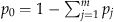 . In the limiting case with an infinitesimal period length, this demand model corresponds to job arrivals generated by independent Poisson processes for the m job types. Researchers have used analogous discrete time demand models with unit arrivals for other revenue and resource management settings (e.g., Kleywegt and Papastavrou 1998, Talluri and van Ryzin 2004).
For the Star flexibility structure, we index the versatile resource type as r=(m+1) and the specialized resource types from 1 to m such that, for r=1, 2, …, m, resource type j is capable of performing only job type j=r. For notational convenience, we omit the subscript t for the resource state, letting 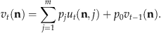
If a type‐j job arrives in period t, the following equation defines the profit‐to‐go function ut
(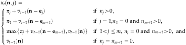
Equation (8) states that, for any incoming job type j, if a type‐j specialized resource is available, the exact policy accepts the job and assigns a specialized resource. Otherwise, if j=1 (i.e., the arriving job is the most profitable type) and a type‐(m+1) versatile resource is available, then the policy accepts and assigns a versatile resource to this job. For j>1, if the type‐j resource is exhausted (i.e., nj
=0) but versatile resources are available, the exact policy accepts and assigns a versatile resource to the type‐j job only if  . Define
  as the marginal value (before observing the demand in period t) of adding one more versatile resource to the resource state
  , i.e., this job's profit margin πj
exceeds the marginal value of a versatile resource at resource state (
, i.e., this job's profit margin πj
exceeds the marginal value of a versatile resource at resource state (
Next, we develop some structural properties of the profit‐to‐go function. First, we can show that vt
(
L
Δ
t
(
 is non‐increasing in nr, for any r=1, …, m, m+1;
 for any r=1, …, m.
P
The results of Lemma 1 have intuitive appeal. Parts (1) and (2) show that the value of an additional versatile resource is lower when more resources are available, i.e., in systems with abundant capacity, or as the end of the decision horizon approaches. Part (3) implies that this resource is worth more in a state containing a specialized resource instead of a versatile resource.
Let  . Since the exact policy accepts a type‐j job only if
  , the definition of
  implies that, if type‐j resources are exhausted, the exact policy assigns a versatile resource to an incoming type‐j job only if
  . The next proposition summarizes the properties of this state‐dependent threshold function
  .
.
P
if the exact policy accepts a type‐j job in state
 is non‐increasing in nk, for any specialized resource type k≠j and fixed t;
 is non‐decreasing in t, for any specialized resource vector
 in period t, then it must also accept this job in state
 in period t, for any specialized resource type k and period t.
P
Since  is non‐increasing in nk, k≠j for fixed t, and non‐decreasing in t for fixed
  specifies a switching curve, or a state‐dependent threshold function, that is non‐increasing in n
1 and non‐decreasing in t.
specifies a switching curve, or a state‐dependent threshold function, that is non‐increasing in n
1 and non‐decreasing in t.
Results analogous to Proposition 2's threshold characterization of the exact policy also arise in other dynamic decision settings. For instance, Lautenbacher and Stidham (1999) prove the optimality of the threshold structure for acceptance decisions in the single‐leg airline yield management problem. More generally, our threshold policy and its monotone structure are consistent with policies for other dynamic decision contexts that are characterized by state‐dependent critical numbers or switching curves (e.g., Puterman 2005). However, no one has previously characterized exact policies for the flexible resource deployment problem with the Star resource structure, and previous results on threshold policies do not directly apply or extend to our problem. Our results regarding the threshold structure of the exact policy also apply to the following generalization of the model. Suppose, for each job type j, the profit margin depends on the resource type (specialized or versatile) assigned to that job type. Let π
j,j
and π
j, m+1 denote, respectively, a type‐j job's profit margin if we assign a specialized or versatile resource to this job. We index the job types so that  . Then, Lemma 1 and Proposition 2 remain valid if
  , for all j, i.e., if we prefer using a specialized resource, if available, rather than a versatile resource for each job type.
The analysis of dynamic resource deployment with the Star resource structure provides some useful policy insights that we can use to address the general flexible resource deployment problem. The time and state‐dependent threshold value  represents the amount of versatile capacity that we wish to reserve for future arrivals of jobs that are more profitable than type‐j jobs; we accept an arriving type‐j job only if the available resources exceed this threshold. We later extend this approach to problems with general flexibility structure by first determining how many resources to reserve for future jobs of each type, and then deciding which specific resource types to hold. The development of the exact policy for the Star resource structure has also highlighted the following characteristics of a “good” dynamic resource deployment policy that we later adapt. The policy: (i) uses less‐flexible (e.g., specialized) resources first before using more‐flexible resources; (ii) favors not using flexible resources for less profitable job types at the beginning of the time horizon, or when the specialized capacity for more profitable job types is low; and, (iii) tends to preserve flexible resources for future use when flexible resource capacity is tight.
4. Approximate Dynamic Resource Deployment Policies
For dynamic flexible resource deployment problems with general resource flexibility structure, since the associated stochastic dynamic program (1) and (2) is difficult to solve even for moderate‐sized problems, we focus on developing good approximate policies. Problems with general flexibility configurations are significantly more difficult than those with special flexibility structures, such as Star or Downward flexibility, due to the lack of a clear hierarchy among resources in terms of their flexibility. For instance, with Downward flexibility, lower‐indexed resource types (using the resource indexing scheme of section 2.2) are more flexible since they can perform all the job types that any higher‐indexed resource type can perform. Therefore, for each accepted job, it is optimal to assign the highest‐indexed available resource type that can perform this job. With general flexibility structures, we do not have such a complete ordering of resource types. Moreover, the value of a resource depends on the tightness of capacity for the different job types that this resource can handle. For instance, if the anticipated demand for type‐3 jobs is high (and there are no available specialized resources for this job type) whereas demand for type‐2 jobs is low, then a flexible resource that can perform type‐1 and type‐3 jobs is more valuable than one that can perform type‐1 and type‐2 jobs even though type‐2 jobs have higher unit profits than type‐3 jobs. Further, due to the arbitrary overlaps in resource capabilities and resource “chaining” effects that we discuss later, using a particular resource for an accepted job affects the remaining capacities not only for the job types that this resource can perform but also for other job types. That is, rather than a single job type having tight capacity or a single resource type being the bottleneck, a group or set of resource types can constitute the bottleneck for an associated set of job types; further, these sets can vary from period to period depending on the demand realizations. Alternative ways to account for these complex interactions lead to different approximation approaches.
We propose three approximate policies—DCA, NCR, and BCR policies—that differ in the principles and methods they use to make job acceptance and resource assignment decisions after observing the demand in each period. Analogous to the threshold criterion of the exact policy for the Star flexibility structure with unit job arrivals, our approximate policies first determine the desired level of capacity to be reserved for future demand. Since we have a choice of alternative flexible resource types that can perform each job type, we must also develop a tentative plan for the future allocation of resources to job types. Our three approaches differ in the methods they use for these two decisions. The DCA policy accounts well for the general flexibility structure, but ignores randomness in future demand. The NCR policy, on the other hand, incorporates demand stochasticity to reserve capacities in nested fashion, but does not fully account for the arbitrary overlaps in resource capabilities. The BCR policy takes into account both demand stochasticity and flexibility structure. The first two policies employ linear programs to assess the match between demand (current and future) and available capacity in order to guide job acceptance decisions, and to choose an appropriate resource to perform each job accepted in the current period. In contrast, the BCR method simultaneously considers job acceptance and resource assignment decisions. We next motivate and develop the three policies; section 5 presents computational results to assess the effectiveness of these policies.
4.1. Preliminaries and Notation
To streamline the presentation of our dynamic resource assignment policies, we introduce some additional notation and terminology. For each job type j∈
As we noted in section 3, whenever specialized type‐sj
resources are available, it is optimal to accept and assign arriving type‐j jobs to these resources. Accordingly, after observing the demand in every period, each of our policies first assigns any available specialized resources to the incoming jobs. Hence, if djt
denotes the actual demand for type‐j jobs and  is the number of available type‐sj
resources at the start of period t, then this initial “Assign and update specialized resources” step accepts
is the number of available type‐sj
resources at the start of period t, then this initial “Assign and update specialized resources” step accepts  units of the incoming type‐j jobs to specialized type‐sj
resources, and updates
units of the incoming type‐j jobs to specialized type‐sj
resources, and updates 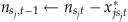 for every job type j∈
 denote the remaining or residual demand for type‐j jobs in period t. With CDjt
denoting the (random) cumulative demand for type‐j jobs from period t onwards, define
denote the remaining or residual demand for type‐j jobs in period t. With CDjt
denoting the (random) cumulative demand for type‐j jobs from period t onwards, define 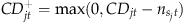 as the residual cumulative demand from period t onwards after we use up all the available type‐sj
specialized resources.
as the residual cumulative demand from period t onwards after we use up all the available type‐sj
specialized resources.
4.2. DCA Policy
The DCA policy addresses the challenge of determining which subset of resource types will jointly constrain future job acceptances by using the expected demand model of section 2.2 to plan a tentative allocation of resource types to current and future demand. This linear program captures well the capacity interactions among resource types within a general resource flexibility structure, but does not consider demand stochasticity. However, from Proposition 1 we know that the optimal value of the expected demand model is an upper bound on the true value function for the stochastic problem. For other stochastic dynamic programming problems, researchers (e.g., Bertsekas and Tsitsiklis 1998, Bertsimas and Popescu 2003) have previously proposed and successfully applied a similar tactic of replacing the true value function with a deterministic approximation obtained by assuming fixed values for the stochastic variables.
For the dynamic flexible resource deployment problem, the DCA policy consists of two main steps in each period t. In the first step, we apply the deterministic optimization model, using the number of residual jobs on hand  plus the expected value of residual cumulative demand
  from the next period (t−1) onwards as type‐j demand. The solution to this profit‐maximizing problem provides a proposed mix of job types to be accepted using the available resources. Since this model combines current and future demands and does not distinguish between using alternative resource types, we employ a second optimization step to decide how many of the current jobs to accept and which resources to assign to these accepted jobs. This latter model uses shadow price information from the previous solution to identify and preserve “valuable” resources for future periods while accepting the same total number of jobs as the resource allocation plan from the first step. A formal description of the DCA policy follows.
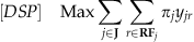
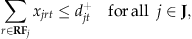
Assign and update specialized resources. Solve the following Demand Selection Problem [DSP], with decision variables yjr
denoting the number of type‐j jobs assigned to type‐r flexible resources in current and future periods. Solve the following Resource Assignment Problem [RAP], using decision variables xjrt
and wjr
for the number of type‐r resources to assign to current and future type‐j jobs, respectively, for all j∈ Let
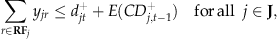

 be the optimal solution to this linear program, and define
 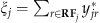 as the total number of type‐j jobs that this solution accepts and assigns to flexible resources from period t onwards. Let σrt
be the optimal shadow price of resource constraint (11) for each resource type r∈
as the total number of type‐j jobs that this solution accepts and assigns to flexible resources from period t onwards. Let σrt
be the optimal shadow price of resource constraint (11) for each resource type r∈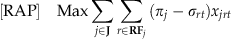


 denote the optimal x‐values for this linear program. For each job type j∈
 current type‐j jobs to type‐r resources, and update the number of available resources for the next period, i.e., set
  , for every flexible resource type r∈
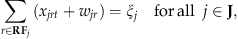
The resource assignment model's objective function (13) maximizes the net profit from jobs accepted this period, where we define the net profit of assigning a type‐r resource to a type‐j job as the profit margin πj
of the job minus the shadow price σrt
of the resource. Constraints (14) and (15) specify that we cannot assign more than  and
and  resources, respectively, to current and future jobs of each type. Constraints (16) are resource capacity constraints, while constraints (17) ensure that the total number of accepted jobs (for current and future demands) for each job type j equals the value ξj
chosen by the optimal solution to model [DSP]. The model judiciously assigns resources to current jobs, preserving resource types with high value (shadow price) for future use. For a problem with m job types and l resource types, we can represent both problem [DSP] and problem [RAP] as minimum cost network flow problems defined over appropriate networks with O(m+l) nodes and O(ml) arcs. The assignment of resources to current jobs in Steps 0 and 2 require O(ml) effort. The overall complexity of the DCA method is governed by the time to solve the network flow problems which is O{(ml)2(m+l)log(m+l)} per period (Orlin 1997). For problems in which job profitability varies with the resource assigned to the job, we can readily adapt the DCA method by replacing the parameters πj
in the objective functions (9) and (13) of the optimization models [DSP] and [RAP] with resource‐dependent profit margins.
resources, respectively, to current and future jobs of each type. Constraints (16) are resource capacity constraints, while constraints (17) ensure that the total number of accepted jobs (for current and future demands) for each job type j equals the value ξj
chosen by the optimal solution to model [DSP]. The model judiciously assigns resources to current jobs, preserving resource types with high value (shadow price) for future use. For a problem with m job types and l resource types, we can represent both problem [DSP] and problem [RAP] as minimum cost network flow problems defined over appropriate networks with O(m+l) nodes and O(ml) arcs. The assignment of resources to current jobs in Steps 0 and 2 require O(ml) effort. The overall complexity of the DCA method is governed by the time to solve the network flow problems which is O{(ml)2(m+l)log(m+l)} per period (Orlin 1997). For problems in which job profitability varies with the resource assigned to the job, we can readily adapt the DCA method by replacing the parameters πj
in the objective functions (9) and (13) of the optimization models [DSP] and [RAP] with resource‐dependent profit margins.
4.3. NCR Policy
For the Star flexibility structure that we analyzed in section 3, the exact policy accepts an incoming type‐j job only if the number of available flexible resources at any period t exceeds a state‐dependent threshold value. This value represents the amount of versatile capacity we wish to reserve to meet the future demand for all the job types that are more profitable than type‐j jobs. The NCR policy extends this approach to general resource structures. Specifically, for each job type j, we first determine the desired total capacity (of all capable resource types) to be reserved for future demand (after period t) of all job types that are more profitable than type‐j jobs, and then determine which specific resource types to reserve. We refer to this capacity reservation scheme as a nested policy since, instead of reserving capacities separately for each job type j, it pools the capacity needed for the more‐profitable job types 1, 2, …, (j−1). Determining the exact threshold function, i.e., optimal capacity reservations, for this nested scheme is an intractable problem. We, therefore, use an approximate newsvendor‐like method to determine the capacity reservations, and then solve an optimization problem to decide which specific resource types to reserve for future demand.
The capacity reservation choice depends on the tradeoff between accepting a current job to capture its profit versus preserving the resource for possible future use to perform a more profitable job. Since this tradeoff is analogous to the balance between overage and underage costs in the traditional newsvendor problem, we use a critical fractile approach to determine the desired capacity reservations. Researchers have previously used the newsvendor principle to develop approximate policies for other revenue management problems. For instance, to allocate a common pool of seats (single resource type) among multiple fare classes (job types), Belobaba (1989) proposed setting the booking limit for each fare class using a newsvendor model.
To motivate our capacity reservation method, we first explore the capacity reservation decision for a two‐period problem with two job types, and three corresponding resource types—specialized type‐1 and type‐2 resources for job types 1 and 2, respectively, and versatile type‐3 resources. In the first period (t=2), after observing the demands for type‐1 and type‐2 jobs, the optimal policy accepts as many type‐1 jobs as possible using available type‐1 and type‐3 resources, and assigns any available specialized type‐2 resources to the incoming type‐2 jobs. Let n
3>0 be the number of remaining versatile type‐3 resources available after these initial assignments. (To simplify the notation, we omit the time index for the state variables.) We wish to determine how many of these n
3 resources to reserve for future type‐1 jobs; this decision will determine how many of the current residual type‐2 jobs to accept and assign to versatile resources (in the first period). Let  denote the residual type‐2 jobs after assigning specialized type‐2 resources. (If
  , then all n
3 versatile resources are carried forward to the next period.) To focus on the tradeoff between using available versatile resources to process current type‐2 jobs versus future type‐1 jobs, we consider the most adverse situation in which only type‐1 jobs arrive in the second period (t=1). Let D
1 denote the unknown demand for type‐1 jobs in the second period, and define
, then all n
3 versatile resources are carried forward to the next period.) To focus on the tradeoff between using available versatile resources to process current type‐2 jobs versus future type‐1 jobs, we consider the most adverse situation in which only type‐1 jobs arrive in the second period (t=1). Let D
1 denote the unknown demand for type‐1 jobs in the second period, and define  as the residual type‐1 demand after assigning the n
1 specialized type‐1 resources carried forward from the first period. For our analysis, we assume that
as the residual type‐1 demand after assigning the n
1 specialized type‐1 resources carried forward from the first period. For our analysis, we assume that  is a continuous random variable, and let
  be its cumulative distribution function. If we decide to reserve Q versatile resources for use in the second period, with
  , then we can accept (n
3−Q) of the residual type‐2 jobs in the first period and assign versatile resources to these accepted jobs. Thus, the maximum expected profit‐to‐go after observing demand in the first period but before accepting any residual type‐2 jobs is
, then we can accept (n
3−Q) of the residual type‐2 jobs in the first period and assign versatile resources to these accepted jobs. Thus, the maximum expected profit‐to‐go after observing demand in the first period but before accepting any residual type‐2 jobs is 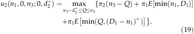
The unconstrained (without resource limits) optimal quantity Q
1 to maximize the expected profit satisfies the classical newsvendor‐type condition  , or
, or 
Accounting for the resource constraints 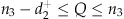 , the optimal number of versatile resources to reserve for type 1 jobs in the second period is
  if Q
1<
if Q
1< , and is min{Q
1, n
3} otherwise.
, and is min{Q
1, n
3} otherwise.
Since extending this characterization of the exact reservation policy to a system with more than two job types and with general resource flexibility structure is analytically intractable, we adapt the approach using some approximations. First, in each period t, we treat the demand during the remaining (t−1) periods as an aggregate demand that occurs in a single future period. Second, analogous to the previous assumption that only type‐1 jobs arrive in the second period, we only consider the future demand for type‐j and more profitable jobs when deciding the capacity reservation for these jobs. Finally, for deciding whether to accept a current type‐(j+1) job, instead of making a separate capacity reservation for each job type that is more profitable than job type (j+1), we determine a combined reservation for all the more‐profitable job types k=1, 2, …, j, effectively treating these job types together as a composite job type with an appropriate weighted average profit parameter, as discussed below. (For airline seat reservations, researchers have distinguished between analogous partitioned and nested booking limits except that these limits refer to allocation of versatile or downward flexible resources whereas we are concerned with determining the desired total capacity, over multiple resource types with arbitrary flexibility structure, to allocate for various job types.) For a multi‐class newsvendor problem, Sen and Zhang (1999) showed numerically that reserving capacity separately for each demand class is inferior to using a combined reservation for all more‐profitable demand classes. Our preliminary computational experiments (not reported here) also confirmed that, for the flexible resource deployment problem, our combined reservation approach yields higher profits than a separate reservation for each job type.
For j=1, 2, …, m−1, let Qj
be the desired number of resources that we wish to reserve for future arrivals of jobs of type‐1 through type‐j. We now discuss how to adapt expression (20) (for Q
1 in the two job‐type problem) to compute Qj
in the m job‐type problem. First, since Qj
will be used to decide whether to accept a current type‐(j+1) job, the “overage” cost or opportunity cost of over‐reserving capacity for future jobs is the profit margin π
j+1 of the current job. Hence, we replace π
2 in (20) with π
j+1. Next, for the two job‐type problem, the value π
1 in expression (20) represents the unit profit margin of the more‐profitable job for which we are reserving capacity. In the context of our approximation, we replace this value with the following demand‐weighted average profit for all the job types that are more profitable than job type ( j+1): 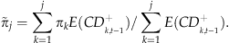
For k=1, 2, …, j, expression (21) uses the expected future residual demand of type‐k jobs from period (t−1) onwards as the weight for the type‐k job's profit margin π
k. Finally, instead of the uncertain future residual demand (D
1−n
1)+ of the single more‐profitable job type (i.e., type 1) in expression (20), we aggregate the future residual demands for all the job types k=1, 2, …, j that are more profitable than job type‐(j+1). Using these principles, we compute Qj
in period t as: 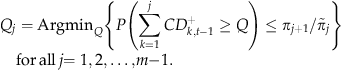
In the context of airline reservations, the expected marginal seat revenue (EMSR‐b) heuristic (Belobaba 1989) uses the same approach to determine protection levels for controlling the usage of a single resource type. Since expression (22) does not consider the currently available resource capacities, we may not have as many resources as we would like to reserve. We therefore refer to Qj
as the aggregate capacity reservation target for type‐j and more profitable jobs. For the two job‐type problem, since we have only a single flexible resource type (i.e., type 3), with n
3 available units, we could easily determine the actual reservation as either  or min{Q
1, n
3}. With general flexibility structure, we have many different resource types that can perform some or all of the job types k=1, 2, …, j. Hence, we face the additional challenge of deciding how many of each specific resource type to reserve for future jobs in order to meet the aggregate capacity reservation target Qj
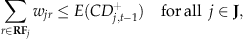
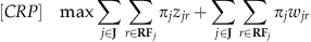
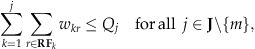
. To account for the actual available capacities, we employ a capacity reservation linear program [CRP] that simultaneously considers the aggregate capacity targets for all j, and attempts to achieve reservations as close as possible to (but not exceeding) the target values, giving preference to reservations for more profitable job types. The NCR policy first solves this linear program to determine the number of jobs of each type to accept in the current period, and later (in the second step) selects the specific resources to assign to the current accepted jobs based upon the resource optimal shadow prices for [CRP]. A formal statement of the procedure follows:
or min{Q
1, n
3}. With general flexibility structure, we have many different resource types that can perform some or all of the job types k=1, 2, …, j. Hence, we face the additional challenge of deciding how many of each specific resource type to reserve for future jobs in order to meet the aggregate capacity reservation target Qj
. To account for the actual available capacities, we employ a capacity reservation linear program [CRP] that simultaneously considers the aggregate capacity targets for all j, and attempts to achieve reservations as close as possible to (but not exceeding) the target values, giving preference to reservations for more profitable job types. The NCR policy first solves this linear program to determine the number of jobs of each type to accept in the current period, and later (in the second step) selects the specific resources to assign to the current accepted jobs based upon the resource optimal shadow prices for [CRP]. A formal statement of the procedure follows:
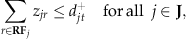
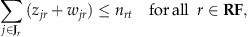
Assign and update specialized resources. Determine the target capacity reservation Qj
using expression (22). Solve the following profit‐maximizing linear program [CRP], with decision variables zjr
and wjr
representing, respectively, the number of type‐r resources to assign to current and future type‐j jobs, for all j∈ Let Set

 be the optimal solution to this linear program.
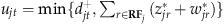 as the number of type‐j jobs to accept in this period. For every flexible resource type r∈
Unlike the DCA algorithm, which uses the expected future residual demand of each job type j to guide planned resource allocations for future demand, model [CRP] reserves resources based on the target aggregate capacity reservation values Qj . The wjr values represent the planned (tentative) allocation of type‐r resources for future type‐j jobs. Since the objective function includes the profits from these allocations, the optimal solution will favor reserving capacity (as much as possible, using the currently available mix of resources) for more profitable job types, subject to the nested reservation limits Qj . Model [CRP] can have alternate optimal solutions that differ in their allocation of capacity between current and future type‐j jobs, for each j. Hence, in Step 2, we first set the number of current type‐j jobs to be accepted, ujt , equal to the smaller of the current residual demand or the total number of resources assigned by the [CRP] solution to type‐j jobs, and then assign less valuable resources, based on resource shadow prices, to these accepted jobs. As in the DCA method, we can represent the optimization model [CRP] as an equivalent minimum cost network flow problem on a network with O(m+l) nodes and O(ml) arcs which can be solved in O{(ml)2(m+l)log(m+l)} time per period. Again, the assignment of resources to current jobs in Steps 0 and 2 require O(ml) effort in total, and so the NCR method has the same computational complexity as the DCA method.
4.4. BCR Policy
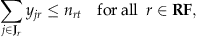
Unlike the DCA policy, the NCR policy considers demand stochasticity when determining the capacity reservation targets Qj to decide whether to accept current jobs. However, by using nested targets, the approach ignores the actual flexibility structure, effectively assuming that a unit of capacity that is not assigned to a current type‐j job can be used to process any of the more‐profitable job types k=1, 2, …, or j−1. But, depending on the resource structure, the acceptance decision for the type‐j job may have no impact on the available capacity for some of these more‐profitable job types, in which case we should not consider the future demand for such jobs when making acceptance decisions for type‐j jobs. Ideally, when considering the use of a type‐r resource for a current type‐j job, we must examine whether this assignment can create or exacerbate a future capacity “bottleneck” for any subset of more‐profitable job types. With general flexibility structures, each job type can be performed by multiple alternative resource types that have arbitrary overlapping capabilities. Hence, bottlenecks are not associated with individual job or resource types, but are rather defined by groups or subsets of job types and the corresponding resource types that can perform any job type in the subset. As we explain below, our BCR policy makes simultaneous job acceptance and assignment decisions based on capacity reservation targets for such bottlenecks.
The BCR policy considers job types j in order of decreasing profitability and resource types r∈ denote the subset of flexible resource types that can perform one or more job types in
  . To compute Q
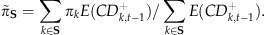
Then, as in expression (22), we define: 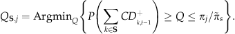
To assess the possible impact of assigning a type‐r resource to a current type‐j job on the available capacity for more profitable job types in the future, we should consider all job subsets  , then we should not assign a type‐r resource to the type‐j job. If none of the <j, r>‐subsets are bottlenecks, then resource type r is a candidate for assignment to a current type‐j job; in this case, we refer to resource type r as a non‐bottleneck resource.
Rather than enumerating every possible subset
Next, we discuss a resource valuation metric that the BCR policy uses to select from among alternative resource types that are available for assignment to a current type‐j job. Define  as an indicator for the tightness of capacity for type‐j jobs. Observe that 0≤θj
≤1 (if at least one currently available resource can perform job type j), with higher values of θ indicating tighter capacity for type‐j jobs. We now define the value of a type‐r resource as
as an indicator for the tightness of capacity for type‐j jobs. Observe that 0≤θj
≤1 (if at least one currently available resource can perform job type j), with higher values of θ indicating tighter capacity for type‐j jobs. We now define the value of a type‐r resource as 
Roughly, interpreting θj
as the likelihood that a type‐j job will be assigned a type‐r flexible resource, the resource value τr
represents the expected profit generated by this resource. This metric accounts for both the profit margins of the job types that a type‐r resource can perform and the capacity tightness for each of these job types. Moreover, it assigns higher value to resources that are more flexible: for any pair of resource types r and r′ with  , the definition (30) of relative value ensures that
  , as desired.
Returning to the overall BCR policy, at each period t, after assigning specialized resources, the method considers job types j=1, 2, …, m in decreasing profit sequence. For each j, the method first attempts to assign resource types r∈ denote these preferred resource types for type‐j jobs. If
Assign and update specialized resources.
Compute the value τr
of each resource type r∈
For j=1, 2, …, m,
For each preferred resource type r∈
Accept  jobs and assign type‐r resources to these jobs;
Update  and
and  .
.
For j=1, 2, …, m,
Set
Step 2.1: For every resource type r∈
construct the flexibility graph GF(j), and determine the job types j′<j that are reachable from resource type r. Let For every job subset
 denote the excess capacity for subset
Let  be the slack for resource r. If bjr
>0, update
be the slack for resource r. If bjr
>0, update  .
.
Step 2.2: If  .
.
Step 2.3: Assign  units of type‐r′ resources to type‐j jobs.
Update the remaining current demand ( ) and resource levels (
 ).
).
If  , go to next job type in Step 2. Otherwise, update the list of non‐bottleneck resources (
 ), and return to Step 2.2.
If j=m, set  for all r∈
By considering all possible subsets of more‐profitable (and reachable) job types at each iteration j of Step 2, the BCR policy generalizes the NCR policy (which considers only one “nested” subset consisting of all job types that are more profitable than type j). In the worst case, Step 2 of the BCR algorithm must enumerate all reachable job subsets for every pair of job and resource types, and hence the complexity of the algorithm is O(2 mml) per period. Although the BCR policy must assess the capacity‐demand match for many more job subsets than the NCR policy, in our computational tests the BCR policy required only a modest amount of additional computational time compared with the NCR and DCA policies. Note that the bottleneck set can change dynamically depending on the demand realizations and acceptance/assignment decisions in each period. The BCR policy accounts for this “shifting” bottleneck phenomenon by recomputing the bottleneck set in every period.
We conclude this discussion of approximate policies by noting that, although we have presented each policy in the discrete‐time setting, these methods also apply when firms need to make job acceptance and assignment decisions as soon as each individual job arrives. Moreover, as we illustrate in section 6, we can also adapt the methods to situations where acceptance decisions are dynamic but resource assignments can be deferred until the end of the decision horizon. Next, we describe our computational experiments and results to evaluate the performance of the three policies.
5. Computational Results
To assess the relative effectiveness of the DCA, NCR, and BCR policies, we implemented and applied them to a wide variety of test problems. We measure the effectiveness of each method in terms of the profit that it generates for each problem instance relative to either the profit for the exact policy (if solving the associated dynamic program [1] and [2] is not very computationally intensive) or the expected PI value (which is an upper bound on the exact profits) for the same problem instance. Since problem difficulty and policy performance depend on various key problem characteristics such as the resource flexibility structure and relative tightness of capacity, we implemented a random problem generator that permits us to systematically vary these characteristics, and designed a comprehensive set of computational experiments to address questions such as the following:
How effective are the approximate policies, i.e., do they generate near‐optimal job acceptance and resource assignment decisions? Is policy performance robust to variations in problem characteristics? Does one of the three policies consistently outperform the others? Can we develop insights on drivers of problem difficulty and decision effectiveness?
Next, we outline our problem generation approach and experimental design. Sections 5.2 and 5.3 discuss computational results, confirming the effectiveness and robustness of our approximate policies to changes in various problem parameters.
5.1. Problem Generation and Experimental Design
We test the performance of different policies over many different problem scenarios, obtained by varying six key problem characteristics that can influence problem difficulty.
The Versatile structure has the highest level of flexibility, and so will yield the largest profit. The relative profitability of the other structures depends on the number of resources of each type as well as the relative demand for different job types. With equal distribution of capacities and demand across resource and job types, the k‐All structure is superior to the k‐Chain structure.
 denote the reward ratio for type‐j jobs relative to type‐(j+1) jobs. We select γj
randomly from a user‐specified interval [γ
min, γ
max]. By varying γ
min and γ
max, we can increase or decrease the relative profit margins of job types. For our experiments, we consider three ranges of reward ratios to capture small, moderate, and large differences in profit margins.
denote the reward ratio for type‐j jobs relative to type‐(j+1) jobs. We select γj
randomly from a user‐specified interval [γ
min, γ
max]. By varying γ
min and γ
max, we can increase or decrease the relative profit margins of job types. For our experiments, we consider three ranges of reward ratios to capture small, moderate, and large differences in profit margins.
The preceding six key problem characteristics, and their associated parameters, provide a convenient framework for specifying problem scenarios. We refer to each combination of settings for the six dimensions as a scenario. In all, our computational study considers 25 different problem scenarios. For each scenario, we randomly generate 10,000 random problem instances, and average the results (relative profits) over these instances to quantify the performance (relative profits) of each policy. To generate a particular problem instance for a given scenario, we first randomly select a value for the capacity tightness index η from [η min, η max], and set the total number of resources equal to ηκ, where κ is the total expected demand of all job types over the decision horizon. Each of these resources is equally likely to be designated as one of the l resource types in the chosen flexibility structure. To determine the profit margin for each job type, we normalize πm =1; then, for j=m−1, …, 1, we randomly select γ j from the interval [γ min, γ max], and set πj =γjπ j+1. Finally, we generate the number of arrivals of each job type in every period t of the decision horizon using the chosen demand distribution. We set κ=60 for all scenarios, and assume that demand is stationary.
For every problem instance, we applied the DCA, NCR, and BCR policies and determined the PI solution by solving the DD model described in section 2.2. For problem instances with three and four job types, we also computed the exact policy (for the problem with general flexibility structure and multiple job arrivals in each period) by solving the dynamic program (1) and (2) using backward induction. Finally, to provide a benchmark for comparing the profits of our optimization‐based flexible resource deployment policies, we applied the following FCFS policy to every problem instance. In each period t, this policy considers job types j in order of decreasing profit, accepting as many of the arriving type‐j jobs as possible using available resources, i.e., the policy accepts  jobs, where nrt
is the number of currently available type‐r resources. To assign specific resources to accepted type‐j jobs, the FCFS method favors using resources r∈
jobs, where nrt
is the number of currently available type‐r resources. To assign specific resources to accepted type‐j jobs, the FCFS method favors using resources r∈
We assess the economic value of each of our approximate policies by comparing their profits with those obtained by the FCFS policy. The profit of the exact policy or the PI upper bound serves to validate the quality of the approximate solutions. We divide our computational results into two sets. In the first set, we focus on determining whether our policies are effective and identifying the best among the three approximate methods. We find that the BCR policy consistently generates near‐optimal profits and outperforms the other policies. Our second set of computations tests the robustness of the approximate policies' performance to variations in problem characteristics such as resource flexibility, capacity tightness, demand variability and balance, relative profitability of jobs, and decision frequency.
5.2. Effectiveness of the Approximate Policies
Our first set of computations seeks to address three main questions: which among our three approximate policies performs best, what benefit do these policies provide relative to the FCFS policy, and does the best policy generate near‐optimal profits? For this purpose, we consider problem scenarios with three to five job types, and various flexibility structures. For problems with three and four job types, we are able to determine the exact policy using dynamic programming, whereas for five job‐type problems, we use the PI upper bound to assess the quality of the approximate solutions. We fix the number of decision periods at T=10, consider moderately tight resource capacities (η∈[0.6, 0.9]) and moderate reward ratios (γ∈[1.5, 2.5]) across job types, and simulate Poisson arrivals with equal expected demand across job types. Such scenarios with balanced demand across job types and equal expected resource capacity for each job type are likely to be the most challenging since all job types have equally tight capacities and contend for flexible resources.
Table 1 summarizes the average optimality gaps between the approximate and exact solution values for problems with three and four job types for various flexibility structures. With three job types (m=3), the 2‐All flexibility structure is the same as the 2‐Chain structure. For problems with more than three job types, to avoid spreading the resources among too many resource types, we do not consider the Complete or (m−1)‐All flexibility structures. We measure the performance of each approximate policy for any scenario as the gap (averaged over 10,000 instances) between the profits of the exact and approximate policies expressed as a percentage of the exact policy's profit.

FCFS, first‐come first‐served; DCA, Deterministic Capacity Allocation; NCR, Nested Capacity Reservation; BCR, Bottleneck Capacity Reservation; PI, perfect‐information.
The results in Table 1 show that all three policies generate good solutions, with optimality gaps of less than 4% for every scenario. (For each scenario, Table 1 shows the smallest gap among the approximate policies in
Comparing the gaps for our approximate policies with those for the FCFS policy reinforces the importance of implementing an optimization‐based policy to guide dynamic resource deployment decisions. The profits generated by the FCFS policy are 14.2% to 28.7% lower than those of the exact policy, and the BCR policy closes over 90% of this gap. The last column of Table 1 shows the percentage gaps between the PI solution values and exact profits. The PI values overestimate the exact profits by as much as 5%, with the PI upper bound becoming weaker as the number of job types increases from three to four. As resource flexibility increases (e.g., comparing the results for 2‐Chain and Versatile resource structures), the PI‐to‐Exact gaps decrease, implying that the exact policy is able to achieve almost as much profit as decisions based on perfect information.
Table 2 reports the results for five job‐type problem scenarios. (For each scenario, Table 2 shows the smallest gap among the approximate policies in
FCFS, first‐come first‐served; DCA, Deterministic Capacity Allocation; NCR, Nested Capacity Reservation; BCR, Bottleneck Capacity Reservation; PI, perfect‐information.
5.3. Robustness of Policy Performance: Impact of Key Problem Dimensions
Having established the effectiveness of our approximate policies, we now study their robustness with respect to the key problem dimensions. For this purpose, we consider variations around a base scenario with three job types, Complete flexibility structure, Poisson arrivals with balanced demand, moderately tight capacity availability η (∈[0.6, 0.9]), moderate reward ratios γ (∈[1.5, 2.5]), and ten periods in the decision horizon. We vary the base scenario, one dimension at a time, to assess the effect on policy performance of capacity tightness, demand characteristics, relative profit margins, and decision frequency. Figure 1 (a–e) displays the percentage gaps, averaged over 10,000 problem instances, between the approximate policies' profits and the exact value for each scenario variant. The results for the base scenario are displayed as grey bars.
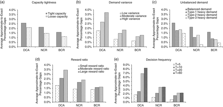
As before, across all the 12 additional scenarios covered by these experiments, the results of Figure 1 show the same consistent pattern of relative performance as in section 5.2: the BCR policy is superior to the NCR policy, which in turn outperforms the DCA policy. For the 12 new scenarios, the average BCR‐to‐Exact gap is only 1.19%, validating the robustness of the BCR policy. We next discuss the results for each of the five scenario variants.
Figure 1(a) compares the gaps for the base case, with moderately tight capacities, and a scenario with moderately loose capacities (η∈[0.9, 1.2]). As capacity increases, more incoming jobs can be accepted, and so we expect the approximate policies to achieve profits closer to the exact profits. Figure 1(a) confirms this performance improvement (reduction in gaps) for the loose capacity scenario. The FCFS‐to‐Exact gap also reduces (to 5.8%) when capacity becomes looser, implying that using our optimization‐based policy is more important when capacity is tight.
Figure 1(b) and (c) address two aspects of the demand process that can affect policy performance— variability in demand and the mix of demand across job types. For the base scenario, with the Poisson demand distribution, the variance of demand equals the mean. To assess the impact of demand variance, we consider three discrete demand distributions that have the same mean as the base scenario (two jobs per period per job type), but different variances. Specifically, we consider scenarios with low variance (1.2), medium variance (2), and high variance (3) using, respectively, a triangular distribution, uniform distribution, and bi‐modal distribution weighted at the extremes. Higher demand variability increases the chances of making erroneous job acceptance and resource assignment decisions. Figure 1(b) confirms this effect, showing that the approximate policies have lower gaps when demand has smaller variation. Turning to the demand mix, our base model assumes that every job type has the same expected demand per period. We are interested in assessing the effect of having unequal expected demand across job types. Varying the relative demand, while keeping the expected number of resources the same for all resource types, introduces variations in capacity availability across job types. We expect this variation to reduce problem difficulty (compared with balanced demand), and so improve the performance of the approximate policies. We consider three unbalanced demand scenarios, one corresponding to each job type j having higher demand than the other two job types. For j=1, 2, and 3, we define the type‐j heavy demand scenario as one in which the expected arrival rate per period is 3 for type‐j jobs and 1.5 for the other two job types (so the total expected demand across all job types is the same as the base scenario). Figure 1(c) confirms our intuition that scenarios with balanced demand are more difficult to solve. The average Approximate‐to‐Exact percentage gaps for the unbalanced problems are significantly lower than those for the balanced problems for all three approximate policies, with the gaps being lowest when the least profitable job type (type 3) has high demand. The FCFS policy has an average optimalicy gap of 7.97% over the three unbalanced demand scenarios. Hence, our optimization‐based policies continue to be valuable for generating higher profits, although less so than with balanced demand.
Figure 1(d) compares the performance of the approximate policies as the relative profitability of job types, captured by the reward ratios, changes. With small reward ratios (γ∈[1.5, 2.5]), job types do not differ much in their profit margins compared with the base scenario with moderate reward ratios, and so the impact of wrong acceptance or assignment decisions on overall profits is lower. In this case, we expect the approximate policies to yield profits that are closer to the exact profits. At the other extreme, with large reward ratios (γ∈[2, 3]), wrong acceptance decisions can have significant profit impact. The results in Figure 1(d) validate this hypothesis; the gaps increase as the reward ratio increases. Notably, however, the BCR policy's performance is robust to changes in the reward ratio, with the gap remaining at less than 1.65% even with high reward ratios. In contrast, the FCFS policy has an average gap of 11.9% for small reward ratios, whereas this gap more than doubles to 27.2% for large reward ratios.
Finally, we study the effect of decision frequency on policy performance. Increasing the decision frequency (by increasing the number of decision periods T in the horizon) permits the firm to be more prompt in its responsiveness to customer requests, but reduces the opportunity to accumulate requests before making acceptance and assignment decisions. To contrast with the base setting of 10 periods, we considered three alternative scenarios with 5, 20, and 60 decision periods, respectively, while keeping the total expected demand in the horizon fixed. As the results in Figure 1(e) show, increasing the number of periods, and hence decision frequency, increases the percentage gap, but only minimally for the BCR policy. The DCA policy's optimality gap more than triples when the decision frequency increases from 10 to 60 (from 2.6% to 8.2%), whereas the BCR policy is much more robust (its gap increases from 1.6% to just 2.2%). The FCFS‐to‐Exact gap increases from 10.9% to 29.3% when the decision frequency increases from 5 to 60. This study also permits us to assess the “cost” of making decisions with less information as decision frequency increases. Figure 1 shows the normalized average profit for the exact, BCR, and FCFS policies as the number of periods T increases from 5 to 60. (We normalize the profits so that the average exact profit for the base case, with T=10, is 100.) The figure also displays the PI value; when T=1 (i.e., single decision period at the end of the horizon), both the exact and BCR policies achieve this value. As expected, the profits of all three policies decrease as decision frequency increases; the figure shows that profit decreases at a decreasing rate with T. Compared with the base case of ten decision periods, doubling the decision frequency (to T=20) reduces the exact profits by 1.8%, while halving the frequency (to T=5) raises profit by 1%. The FCFS policy's performance deteriorates significantly as the number of periods grows; its profit gap relative to the exact policy increases from 16.5% to 29.3% when T increases from 10 to 60, whereas the BCR policy's gap is relatively flat.
To summarize, in this section, we have covered a wide range of problem scenarios to capture many different operating conditions of a firm. Remarkably, the BCR policy always achieves profits that are within 2.2% of the exact policy's profits, and in many cases attains optimality gaps well below 1%. For problems with three or four job types (for which we have the exact profits), over the 19 corresponding problem scenarios (covered in Table 1 and Figure 1), the BCR policy has an average optimality gap of 1.3% (relative to the exact profits), while the NCR and DCA policies have gaps of 1.7% and 3.2%, respectively. The FCFS policy, on the other hand, has an average optimality gap of 18.8% over the same set of problem scenarios. Our experiments have confirmed that contextual features such as moderately tight capacities, high reward ratios, and balanced demand increase problem difficulty.
6. Deferred Resource Assignments
Thus far, we have addressed the situation when both job acceptance and resource assignment decisions must be made dynamically, i.e., in each period, the firm must not only decide which incoming jobs to accept, but also which resource to assign to each accepted job. This model is appropriate for the workplace learning context since clients (and instructors) prefer to know which instructor will conduct their training program soon after their request is accepted in order to begin working on any program customization, plan logistical arrangements, and so on. Other contexts may require only prompt (i.e., dynamic) acceptance decisions, but may not require immediate resource commitments. That is, in each period, the firm only needs to decide which incoming jobs to accept, and can defer the assignment of a specific resource to each accepted job until the end of the horizon (before performing the service). Having the option to defer the resource assignment decisions can increase profits (compared with dynamic assignment decisions) since this option enlarges, albeit modestly, the feasible acceptance region in later periods. 2 We note that the profit with deferred assignment cannot exceed the PI value, i.e., the profit when both acceptance and assignment decisions can be deferred until the end of the horizon.
In this section, we seek to address the following related questions. Can we readily adapt our previous dynamic acceptance and assignment policies to the dynamic acceptance‐deferred assignment model? How effective and robust is the performance of these modified policies for the revised model? What is the economic value (i.e., incremental profits) of deferring assignments compared with dynamic assignments, and how does this value depend on the problem characteristics? To explore these issues, we first (in section 6.1) formally define the revised model by discussing its stochastic dynamic programming formulation. We then illustrate (in section 6.2) how to adapt the approximate policies to handle deferred assignments by describing modifications to one policy—the BCR policy—and report (in section 6.3) computational results for various problem scenarios comparing the profit performance of this modified policy with the profits generated by the exact policy with and without deferred assignment.
6.1. Model Formulation for Dynamic Acceptance‐Deferred Assignment Problem
To formulate the deferred assignment model, we first note that, since resources are not committed until the end of the horizon, the state of the system in each period must specify the number of jobs of each type accepted until that period (instead of the number of remaining unassigned resources for the dynamic assignment model). For t=T, …, 1 and j∈ t
={ζ1t
, ζ2t
, … ζ
mt
}. By definition,
t
={ζ1t
, ζ2t
, … ζ
mt
}. By definition,  T+1=0 and
  1 is the vector of total acceptances over the entire planning horizon. As before,
  t+1,
t+1,
In each period t, we must ensure that the number of new type‐j jobs accepted in this period, say, gjt
for all j∈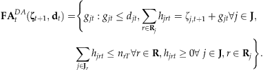
The constraints ensure that: (i) the number gjt
of type‐j jobs accepted in period t does not exceed the demand djt
observed in the period; (ii) the total number of type‐j jobs tentatively assigned to resources equals the number previously accepted (
Now, let  be the maximum expected profit‐to‐go in period t at the current state (
 ,
,  jobs before period t, the value function is
  , where P (
 as
as 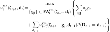
In the last period (t=1), after determining
6.2. BCR Policy with Deferred Resource Assignments
We can modify all three approximate policies of section 4 to handle deferred rather than dynamic resource assignments. To illustrate the needed changes, we modify the BCR policy to handle deferred assignments and report computational results using this modified policy, which we call the BCRDA policy. The BCR policy's strength lies in its ability to dynamically identify resource and job subsets that together constitute capacity bottlenecks taking into account stochasticicy of future demand and the flexibility structure of currently available resources. These bottlenecks then guide decisions on which jobs among the new arrivals in this period to accept. However, while the method accepts new jobs only if the system has adequate capacity to process these jobs, it requires as input the “remaining” resources of each type after assigning to previously accepted jobs to ensure feasibility of these acceptance decisions. For the context with deferred assignments, we have the opportunity to reallocate (tentatively) the resources among accepted jobs in each period. We, therefore, augment the original BCR policy (section 4.4) with a third step, after all acceptance decisions in a period, to reassign resources and determine the remaining resources for new assignments in the next period. Specifically, at the end of Step 2 of the previous BCR procedure for period t, the total number of newly accepted type‐j jobs in this period is  . Hence, the total number of accepted type‐j jobs up to and including this period is
  for all job types j∈
 and
and  to denote the remaining number of accepted type‐j jobs and remaining number of type‐r resources as we assign specialized and preferred resources.
Step 3.1: For j=1, 2, …, m, assign as many type‐j jobs to specialized resources as possible, i.e., set  and
and  .
.
Step 3.2: For j=1, 2, …, m, assign preferred resources. That is,
For resource types r∈ and update
  .
.
Step 3.3: Let  be the set of job types with remaining accepted demand, and
  be the set of flexible resources types with remaining resources capable of performing job type j∈
 .
. 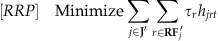
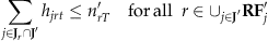

Set  if
if  for some j∈
 otherwise.
The [RRP] model assigns remaining flexible resources to the remaining accepted demand (after assignment of specialized and preferred resources) so as to minimize the value τ r of the resources used. The objective function (32) minimizes this value, while constraints (33) and (34) specify, respectively, that resources must be assigned to all the remaining accepted demand for each job type, and the number of resources assigned must not exceed the number of remaining resources for each resource type r. The BCRDA policy consists of applying steps 1 and 2 of the BCR policy (section 4.4) followed by the above Step 3 at each period t=T, T−1, …, 1. Next, we discuss computational results using this policy for the flexible resource deployment problem with deferred assignments.
6.3. Computational Results for Deferred Assignment Model
To assess the value of deferring resource assignment decisions and validate the effectiveness of the approximate policy, we implemented the ExactDA and BCRDA policies, and applied them to test problems obtained using our problem generation framework of section 5. We expect the ExactDA policy's profit to be higher than that of the previous exact policy with dynamic assignments but lower than the PI solution value. We first explore these profit gaps for the different scenarios introduced in section 5.3. As before, we use the three job‐type problem with Complete flexibility structure, Poisson arrivals, 10‐period decision horizon, and moderate capacity tightness and reward ratios as the base scenario. We consider variants of this base model to study how the flexibility level, capacity tightness, demand variance, demand mix, relative profitability, and decision frequency affect the benefits of deferred assignments. Table 3 compares the average gap (for 10,000 instances) between the PI value and exact profits with the gap between the ExactDA and exact profits for various scenarios; both gaps are expressed as percentages of the exact profits.

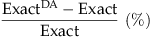
PI, perfect‐information; DA, deferred assignment.
Since the PI solution assumes that both acceptance and assignment decisions can be made after observing the demand for all T periods, the PI‐to‐Exact gap measures the percentage improvement in profit if we can defer both job acceptance and resource assignment decisions to the end of the horizon. On the other hand, the ExactDA‐to‐Exact gap represents the profit improvement when just resource assignments are deferred to the end. On average, over all scenarios, deferring the assignment decision increases profit by only 1% compared with the 2.1% increase when both acceptance and assignment decisions are deferred. However, deferring assignments can be attractive in certain scenarios. Specifically, when demand has high variance, reward ratios are large, or decision frequency is high, deferring resource assignment decisions captures more than 50% of the total profit increase that a firm can realize by deferring both acceptance and assignment decisions. This finding is not surprising since dynamic decisions are likely to reduce profits the most under these three extreme scenarios.
Next, we test the effectiveness of the BCRDA policy, in terms of its near‐optimality, for scenarios with three and four job types. Table 4 presents the average gap between the ExactDA and BCRDA profits, as a percentage of the ExactDA profits, for various flexibility structures. To facilitate comparison with the performance of the original BCR method (without deferred assignment), the last column of Table 4 reports the corresponding Exact‐to‐BCR gaps (previously reported in section 5.2). The average ExactDA‐to‐BCRDA gap over all scenarios is only 1.3%, which is slightly lower than the previous average Exact‐to‐BCR optimality gap of 1.4% for the original BCR policy applied to the same problem scenarios but with dynamic assignments. These results suggest that the BCR policy continues to be effective in generating near‐optimal solutions when adapted to problems with deferred assignments.
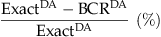
BCR, Bottleneck Capacity Reservation; DA, deferred assignment.
7. Conclusions
Employing a mix of flexible and specialized resources permits firms to broaden their service offerings while maintaining high resource utilization and reducing lost sales. Prior work on the benefits of flexibility largely assumes that resource assignments can be deferred until all the demand is realized, but this assumption may not apply to service firms that must dynamically decide whether to accept incoming jobs, and what resource to assign to accepted jobs. Since these decisions greatly influence the profitability of the enterprise, realizing the potential benefits of flexibility requires a principled approach for dynamic resource deployment.
To our knowledge, this paper is among the first to study the dynamic demand selection and resource assignment problem for general resource flexibility structures. Our analysis of the special case with unit arrivals and the Star resource structure revealed that the exact policy has a threshold structure. Our three approximate policies provide alternative ways to compute and incorporate threshold principles for more general settings. The DCA policy accounts for the capacity interactions with general flexibility structures, but uses expected values as demand estimates. The NCR method accounts for randomness in demands, using a newsvendor‐type approach to determine aggregate capacity reservations, but simplifies the resource structure and interactions among job and resource types. The BCR policy combines the strengths of the previous policies by identifying subsets of resources that are bottlenecks and appropriately reserving capacities. These policies are readily adaptable to immediate decision‐making, as each job arrives, as well as for contexts that permit deferred assignment decisions.
Our extensive computational results demonstrate that the BCR and NCR policies are very effective in generating near‐optimal solutions over a wide range of problem settings, both with dynamic assignments and deferred assignments. The BCR policy's exceptional performance suggests that contexts with general resource flexibility structures require accounting for both demand stochasticity and shifting bottlenecks. The results also show that using simplistic rules such as FCFS can result in significant profit degradation. Our study of the impact of decision frequency on profit performance reveals that assuming perfect demand information for resource deployment, as in most capacity planning models, can lead to considerable overestimation of profits for service contexts that require dynamic and frequent decisions with incomplete information. This observation raises the interesting opportunity for future research on more refined flexible capacity planning models that explicitly incorporate dynamic or multi‐period resource deployment decisions to assess the profitability of candidate capacity investment decisions.
Footnotes
Appendix
1
2
In general, we can consider a spectrum of “partially” deferred assignment models, parameterized by a deferral period td >1, in which assignment decisions for jobs accepted before period td (i.e., for t>td ) can be deferred until td , but the firm must simultaneously decide both acceptance and assignment for t<td . As td becomes smaller, profits increase. We focus on the limiting case with td =1 in order to assess the maximum possible benefits due to assignment deferrals.