Intelligent Procedures for Intra‐Day Updating of Call Center Agent Schedules

Abstract

For nearly all call centers, agent schedules are typically created several days or weeks before the time that agents report to work. After schedules are created, call center resource managers receive additional information that can affect forecasted workload and resource availability. In particular, there is significant evidence, both among practitioners and in the research literature, suggesting that actual call arrival volumes early in a scheduling period (typically an individual day or week) can provide valuable information about the call arrival pattern later in the same scheduling period. In this paper, we develop a flexible and powerful heuristic framework for managers to make intra‐day resource adjustment decisions that take into account updated call forecasts, updated agent requirements, existing agent schedules, agents' schedule flexibility, and associated incremental labor costs. We demonstrate the value of this methodology in managing the trade‐off between labor costs and service levels to best meet variable rates of demand for service, using data from an actual call center.

Keywords

call center operations doubly stochastic processes workforce scheduling integer programming real‐time optimization

1. Introduction

Effective and efficient operation of a telephone call center is largely dependent on strong workforce planning and management (Cleveland and Mayben 1997, Mehrotra 1997), as typically 60–80% of a call center's budget is spent on labor costs. As illustrated in Figure 1, this workforce planning and management involves three levels of decision‐making: long‐term planning, short‐term scheduling, and real‐time schedule adjustments (Abernathy et al. 1973). Long‐term planning decisions address how many agents to hire and train at what times. These decisions are typically made 6–12 months ahead of time and take into account aggregate call forecasts, agent availability and productivity assumptions, and anticipated staff attrition rates. Short‐term scheduling decisions determine which agents are assigned to work on which shifts on which days at which times over the course of a scheduling period (typically 1 week). In most call center environments, scheduling is typically done 1–2 weeks ahead of time, with schedules communicated to individual agents so that they can plan accordingly. Scheduling decisions are based on estimated agent requirements (which in turn are based on detailed forecasts for call arrival patterns and service times as well as customer waiting time goals), shift definitions and restrictions, agent rosters and shift preferences, and absenteeism assumptions.

Figure 1

Three‐Level Hierarchical Model of Call Center Resource Planning

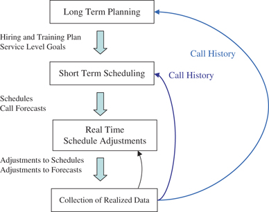
By contrast, real‐time schedule adjustments are made after agents have been hired and trained, agent schedules have been created, and additional details have become available about call volumes, absenteeism, and unanticipated off‐phone activities such as training and meetings. Adjustments are then made on an intra‐day basis to agents' schedules. There is typically a limited set of feasible adjustments that can be made due to human resource policies and practices (see table 2 of Easton and Goodale 2005, for a good overview).

There is a substantial and growing body of academic research on call center workforce management (Aksin et al. 2007, Gans et al. 2003). The vast majority of this research focuses on call forecasting, queueing, and short‐term scheduling, with a small amount of work on long‐term planning. Very little attention has been devoted to the issues and decisions associated with real‐time schedule adjustments, either for call centers or for other types of service systems.

However, there are several factors that make real‐time schedule adjustments vital for successful call center management. Most importantly, several researchers (Avramidis et al. 2004, Brown et al. 2005, Jongbloed and Koole 2001, Shen and Huang 2008, Steckley et al. 2004, Weinberg et al. 2007) have recently identified significant correlation between arrivals in different time intervals within the same day, and have suggested methods for updating call forecasts on an intra‐day basis; a primary purpose for such updated call forecasts is to provide support for real‐time schedule adjustments. Secondly, given the lead time associated with schedule generation, many changes to employee availability can and do take place after the original schedules have been created. Thirdly, detecting how well the scheduled agent workforce actually matches the actual workload is often not possible for a given day until that day has begun, at which point responding to the incremental (positive or negative) demand may be crucial. Finally, managers regularly struggle with staffing tradeoffs, for while having too few agents on duty can lead to severe degradations in service quality, having too many agents results in low resource utilization and overspending of scarce financial resources.

The task of making intelligent real‐time schedule adjustments is a challenging undertaking. Managers have many possible ways of increasing staff levels (offering overtime to agents already scheduled to work, calling in additional agents from home or “borrowing” resources from another department, utilizing outsourcers, eliminating off‐phone activities such as meetings or trainings) or decreasing total agent on‐phone hours (offering voluntary time off [VTO], moving agents to other activities or queues). All of this—when combined with multiple time periods, multiple agent types and costs, and broad classes of feasible shift change options—results in substantial combinatorial complexity.

Despite this complexity, recent empirical research (Mehrotra et al. 2009) estimates that over 70% of call centers routinely make real‐time schedule adjustments, with these decisions based largely on experience and intuition. Typically, actual agent attendance and call volumes are observed and compared with forecasted values during the early part of the day, and then agent schedules are updated in an ad hoc manner based on these observations.

The objectives and main contributions of this paper are as follows: (1) to develop a new mathematical framework for real‐time schedule adjustments that reflects the operational characteristics of the call center environment; (2) to connect the growing literature on random arrival rates and inter‐period correlations for inbound call centers to the problem of agent re‐scheduling; (3) to identify and illustrate a tractable solution methodology for updating forecasts and determining cost‐effective schedule adjustments based on these updates; and (4) to illustrate the impact of making these real‐time schedule adjustments on operating costs and service quality.

In section 2, we describe the real‐time management challenge in more detail and review the relevant research literature. In section 3, we present a framework for managing real‐time schedule adjustments within call centers, including a workload forecast updating model and an integer programming formulation that reflects the costs and constraints associated with adjusting agent schedules on an intra‐day basis. In section 4, we demonstrate the value of using this framework to update schedules through an illustrative set of numerical examples. Finally, in section 5, we conclude by discussing the importance of real‐time monitoring and management in call center operations as well as directions for future research.

2. Review of Call Center Workforce Management Processes and Associated Literature

Throughout this paper, we focus on call centers in which all calls are inbound calls from customers and all agents are capable of handling all calls. In such call centers, as in many labor‐intensive industries (Hur et al. 2004), the essential scheduling challenge faced is cost‐effectively matching the actual demand for service with the service delivery resources (which we refer to as “agents”) available to handle this workload.

The actual workload faced by an inbound call center is typically modeled as a stochastic process based on a random number of arriving calls and a randomly distributed service time for each call. Therefore, the forecasting of workload is an important part of the agent scheduling (and re‐scheduling) process. There is extensive literature in this area that is well reviewed by Gans et al. (2003) and by Aksin et al. (2007). In particular, Thompson (1998) provides a general tutorial on demand forecasting for service systems while Andrews and Cunningham (1995) present a vivid case study of one call center's forecasting challenges.

Within the call center literature, the standard forecasting approach is to treat call arrivals over the course of a day or week as a non‐homogeneous Poisson process (NHPP) with piecewise constant arrival rates over specific time intervals of 15, 30, or 60 minutes that are independent of each other. Indeed, there is significant theoretical and empirical evidence that supports the concept of modeling call arrivals as an NHPP. When one considers call arrivals as the superposition of arrivals from a large number of independent customers, the Palm–Khintchine theorem shows that a Poisson process provides a good approximation (Whitt 2002). As part of an extensive empirical analysis of one call center's data, Brown et al. (2005) report that they could find no evidence to reject the hypothesis that call arrivals follow an NHPP.

The typical next step is to translate the forecasted arrival rates into a demand for agents, which depends not only on the workload forecast but also on a defined acceptable waiting time distribution. Grassman (1988) discusses many of the practical issues generally associated with this type of translation, while Green et al. (2001, 2003) describe the standard call center forecast translation process, which they refer to as the stationary, independent, period by period (“SIPP”) method. The SIPP method treats each individual period as an independent stationary queueing system, and for each period sets the target number of servers to be the minimum number for which the acceptable waiting time distribution will be achieved in steady state, given the workload forecast. Green et al. (2001, 2003) also propose improvements to the way in which agent requirements are determined for call centers with cyclic demand (2001) and call centers with limited daily operating hours (2003).

The translation of call arrival forecasts and target waiting time distributions into agent requirements depends implicitly on the assumption that the forecasted call arrival rates are known and deterministic. However, recent research has also shown that the assumption of a deterministic arrival rate within a given period is often invalid, which has implications for determining the number of agents to schedule in each period. Brown et al. (2005), studying data from a bank's call center, test and reject the hypothesis of deterministic (Poisson) arrival rates per time period. Similarly, Steckley et al. (2004) analyze data from several call centers' queues, statistically testing and rejecting the hypothesis that arrival rates are deterministic for the vast majority of queues and time periods studied. Whitt (1999) examines infinite‐server systems as a mechanism for understanding the staffing levels required for systems in which the objective is to answer calls immediately, while Whitt (2006) also considers both random arrival rates and employee absenteeism (along with costs associated with servers, waiting time, and abandonment) in developing approximation techniques for determining the optimal number of servers for a given workload distribution. Steckley et al. (2009) provide approximation techniques for performance measures associated with waiting time distribution in the presence of a random arrival rate in order to facilitate the selection of the number of servers. Motivated by empirical observations of random arrival rates, Jongbloed and Koole (2001) consider the question of how to “schedule agents … in a statistically correct way” when the arrival rate itself is a random variable. In particular, they propose a Poisson mixture model for arrivals within a specific time period, and then explore various methods for determining the number of agents to schedule. Robbins (2007) suggests a stochastic programming approach to scheduling agents while explicitly accounting for arrival rate uncertainty.

In addition to random arrival rates, there is also considerable evidence that the arrivals across different periods within the same day or week are correlated with one another; these correlations have in turn prompted researchers to create more sophisticated forecasting and staffing models. Motivated by empirical results that show strong correlations across periods within the same day, Avramidis et al. (2004) develop and test several models in which the arrival rate for each interval of the day is a random variable that is correlated with the arrival rates of the other intervals. Brown et al. (2005) develops a non‐linear least‐squares model in which a previous day's call volume is an independent variable in predicting the subsequent day's call volume, producing roughly a 50% reduction in the variability of the forecasted daily volumes.

Most recently, several researchers have confirmed the persistent presence of intra‐day cross‐period correlations in large call center datasets and developed sophisticated techniques for intra‐day forecast updating. Weinberg et al. (2007) use data from a large North American bank to develop a two‐way multiplicative Bayesian Gaussian model for forecasting call arrivals, with Monte Carlo Markov Chain (MCMC) methods used for parameter estimation; their empirical analysis shows strong intra‐day correlations and substantial improvements in forecast accuracy based on MCMC parameter updating. Shen and Huang (2008) analyze data from a major financial services firm's inbound call center and demonstrate strong intra‐day correlations; these results are used to motivate intra‐day forecast updating methods based on singular value decomposition techniques and a penalized least‐squares model.

Beyond call centers, this intra‐period correlation has been investigated in many other settings as well. Bodily and Freeland (1988) examine several different forecast updating techniques for predicting overall product shipments based on initial observed orders, while Kekre et al. (1990) and Guerrero and Elizondo (1997) also examine the problem of updating a cumulative demand forecast based on a subset of actual demand. Hur (2002) proposes a variety of monitoring techniques to identify when new information might suggest the need to update previous forecasts.

These recent research results support the premise that new information about call arrivals during the first few time intervals of a given day may provide important insights into the distribution of calls over the remainder of the day, and in turn provide motivation for adjusting agent schedules in order to better meet an updated demand forecast.

Real‐time schedule adjustment processes start with initial forecasts and agent schedules, and then seek to update them based on new information that has become available more recently. The three components of the re‐scheduling process are analogous to the three components of the scheduling process, and thus the literature on real‐time schedule adjustments includes work on: (1) updating call forecasts; (2) revising resource requirements; and (3) updating agent schedules.

Interestingly, while there is great deal of literature on shift scheduling in general (Ernst et al. 2004) and in call centers in particular (Aksin et al. 2007, Gans et al. 2003), real‐time schedule adjustments have been studied far less extensively. Thompson (1996, 1999) has done some initial work on real‐time schedule adjustments in service systems. Easton and Goodale (2005) propose a methodology for re‐scheduling resources in service systems to account for absenteeism, focusing on systems in which there is quantifiable marginal revenue associated with handling customers that would otherwise abandon the system. Hur et al. (2004) provide an excellent overview of the literature associated with real‐time schedule adjustments while highlighting some of the challenges and also developing re‐scheduling techniques specifically for the context of quick service restaurants. Citing several sources, including Cleveland and Mayben (1997) and Mabert (1991, 1995), Hur et al. (2004) also assert that “even the most accurate call center staff scheduling must be complemented by real‐time schedule adjustment to achieve the target customer service level.” Despite this widespread belief, there is a surprising absence of research on real‐time agent schedule adjustments within the call center research literature.

3. Intra‐Day Schedule Updating Methodology

3.1. Overview

In this section, we describe our Intra‐Day Schedule Updating methodology. The underlying business context is a (possibly virtual) call center that handles a single type of incoming phone call, with all agents being skilled to handle each call. At the beginning of the day, there is an initial call volume forecast for each period of the day, and an existing set of agents who are scheduled to handle this workload. Agents are grouped into “types” by the specific details of their schedules, where an agent type is defined by (a) the period in which agents of this type begin their shift; (b) the specific periods during which they are available to handle calls; and (c) the period in which they complete their shift.

Once the day begins, managers observe the actual workload (and the actual attendance of the agents) at the end of each period, paying attention to the deviation from the forecasted workload (and the expected agent coverage levels). When the cumulative call volume deviates significantly from what was forecasted, the forecast for the remainder of the day is updated, an incremental demand for agents for each period for the remainder of the day is identified, and some or all agents' schedules can be updated to reflect these changes in demand. If the value of these schedule changes exceeds the associated disruption costs, the schedule changes are communicated to agents and the updated schedules are followed for the remainder of the day.

Once the incremental demand for agents has been identified for subsequent periods of the day, the intra‐day rescheduling model seeks to identify a cost‐effective solution that meets the updated agent requirements for each remaining period. To accommodate this rescheduling, agents of a particular type may be asked to transition to a different schedule, with this new schedule featuring at least one period in which this agent was previously working (or idle) but is now idle (working). It is assumed that the range of possible new schedules for each agent type, the costs associated with each of these transitions, and the disruption costs associated with changing agent schedules are all known before solution of the re‐scheduling problem.

3.2. Initial Schedule Parameters and Notation

To represent the call center's daily operations and initial agent schedules, for a given day we define the following notation:

Initial Parameters

T=	number of periods within a day
N =	number of agent types
m_i =	number of type i agents originally scheduled to work on this day
b_it =	1, if type i agents are scheduled to take inbound calls in period t; 0, otherwise, for i=1, 2, … , N and t=1, 2, … , T
d_t =	number of agents scheduled to take inbound calls in period t, for t=1, 2, … , T

For any given vector m={m_i } and matrix B={b_it }, we can compute d={d_t } using d=Bm.

The case where b_it =0 for all corresponds to all agents of type i being currently unscheduled for the particular day in question. In practice an agent of this type may be someone who is available to be called in from home with some lead time, an employee in another department who is capable of handling these calls, or an agent who is available from a third party or “outsourced” call center (see Easton and Goodale [2005] for a good discussion of these types of contingent resource options). For this type of agent, the parameter m_i corresponds to the maximum number of agents of this type who are available for duty as part of an updated agent schedule.

3.3. Monitoring Call Volumes and Identifying Incremental Demand for Agents

Before each time period u, our methodology monitors actual call arrivals and compares them to forecasted call volumes. When the cumulative call volume deviates significantly from the expected cumulative call volume, we identify u as a possible schedule updating period and estimate an incremental demand for agents. This incremental agent demand then serves as an input into the agent rescheduling model described in section 3.4. Our description below uses the following notation and associated definitions:

Agent Demand Updating: Definitions and Notation

N_t =	random variable representing the number of calls arriving in period t
λ_t =	expected value of N_t
C_u =	random variable representing the cumulative number of calls arriving in periods 1, 2, … , u−1
x_t =	actual number of calls observed in period t, for t=1, 2, … , u−1
S_u =	actual cumulative number of calls arriving in periods 1, 2, … , u−1
=	number of agents required to take inbound calls in period t after the updated forecast, for t=u, u+1, … , T
δ_t =	the amount of staff change justified by the updated forecast and observed agent attendance levels in period t, for t=u, u+1, … , T

3.3.1. Modeling Call Arrivals. We model N_t as a stochastic process with random arrival rates in which the number of calls arriving in each period may be correlated with the number of calls arriving in previous periods. This general model allows for a wide range of call forecasting techniques, including the distributional forecasting models presented in Whitt (1999), Brown et al. (2005), Avramidis et al. (2004), Weinberg et al. (2007), and Shen and Huang (2008).

3.3.2. Comparing Actual Call Arrivals to Forecasted Call Arrivals. Our first criterion for determining whether or not to adjust agent schedules at the beginning of a given period u is to compare actual calls with the distributional call forecasts. Immediately before period u, we monitor the actual cumulative call arrivals S_u . Given the distributional forecasts for the call volumes N ₁, N ₂, … , N _u−1, we also have a distributional forecast for the cumulative call volume C_u for periods 1, 2, … , u−1. Based on the distributional forecast for C_u , we can compute . We interpret a small value (respectively, a large value) of π _u to suggest that the actual cumulative call volume is significantly greater than expected (significantly lower than expected). Our methodology utilizes threshold values p ₁ and p ₂, where , to determine whether the call center is potentially overstaffed (if ) or potentially understaffed (if ).

On the other hand, we infer that S_u is relatively close to E[C_u ] if , and consequently we do not consider updating agent schedules before period u. In such cases, the remaining steps described in the sections below are not executed for period u.

3.3.3. Updating Forecasts Based on Actual Call Volumes S_u . If the call center appears to be overstaffed or understaffed based on the criteria described in the previous section, the next step in our methodology is to update the forecasts. This is defined quite generally, and can be either an update to the forecasted mean arrival rates λ_t for t=u, u+1, … , T (which we denote ) or an update to the distributional forecast for N_t for periods t=u, u+1, … , T (which we denote ). In either case, the purpose of the updated forecast is to determine an updated target for agent requirements, which we discuss in the next section.

3.3.4. Updating Target Agent Requirements and Incremental Per Period Agent Demand. Given an updated forecast for the call arrival rates , one can use the standard SIPP translation or one of several variants in the literature (as discussed in Green et al. 2001) to determine the value of , the minimum number of agents needed to achieve the desired waiting time objective in periods . Alternately, the additional information contained in the updated distributional forecasts for periods can be used to determine using approximation techniques such as those presented by Steckley et al. (2009). Throughout the remainder of this section, we suppress the superscript on for clarity.

Next, for all periods t≥u, we compute where the first term on the right‐hand side corresponds to the target number of agents for period t based on the updated forecast and the second term corresponds to the number of agents originally scheduled for period t.

For clarity of exposition, we have omitted any adjustment for absenteeism in our description of the methodology here. However, absenteeism can be incorporated simply by adjusting the number of scheduled agents d_t by the number of scheduled agents who as of the end of period u−1 are projected to be absent during each period before computing the δ _t values for all periods t≥u. Similarly, although our presentation above focuses on changes in call volume forecasts, we note that changes to service time parameter forecasts and/or the waiting time distribution (“service level”) objectives for the remaining periods can also be considered in a straightforward manner.

3.4. Formulation of the Re‐Scheduling Model

Once the change in agent demand δ_t has been determined, we then solve an integer programming model to determine a cost‐effective agent re‐scheduling plan. This model is formulated in detail in this section, first in general terms and then for two important special cases.

Schedule Updating Parameters

K_i =

number of schedule transitions available to a type i agent

Cost and Saving Parameters

p_ik =	the penalty of making the transition k for a type i agent
	the cost of having a type i agent make a transition in period t where r_ikt =1
	the savings from having a type i agent make a transition in period t where r_ikt =−1

Decision Variables

y_ik =

the number of type i agents who transition to the new schedule k

The general schedule updating model determines the number of agents of each type that should make each type of feasible transitions in order to accommodate the forecast update while minimizing the total cost of the transitions. Mathematically, the objective is to Subject to 1 2 3

3.4.1. Special Case I: The Understaffed Call Center. In the intra‐day context, we describe a call center as being “understaffed” if and for at least one period after the forecast update in period u. When a call center is understaffed, management is confronted with a difficult choice: maintaining current staffing levels is likely to result in long waiting times and high abandonment rates, while increasing staffing levels means additional labor expenditures. In such cases, our modeling framework seeks to enable managers to improve service quality while at the same time cost‐effectively managing incremental labor costs.

One way to increase the staffing levels is by extending one or more agents' shifts by one or more periods; this extension of an agent's shift is known as “overtime” (OT) and typically has a pay premium associated with it. In this case, we assume that an agent who is done with his regular shift immediately starts working overtime if he is offered OT. Another way to increase staffing levels is to add agents who are not already scheduled to handle these calls, either by calling in agents from home, from another department or group, or from an outsourcer. The challenge is to determine how many of each type of resource to add to the schedule over which periods of the day.

We now present an integer programming model to determine a cost‐effective mix of OT offers and additional agents (how many agents and for what periods) to remedy the understaffing that is projected for periods . For clarity of exposition (and without loss of generality), we will assume that u=1 for the remainder of the model section.

For this special case, we will need the following additional notation:

Parameters for the Understaffed Model

o_i =	overtime cost per period of a type i agent
p_it =	cost of making a schedule change to a type i agent in period t
e_i =	daily cost of bringing in a call‐in agent of type i
L_i =	The last period in which a type i agent is on staff with regard to his original schedule

Decision Variables for the Understaffed Model

Y_it =	the number of type i agents that work overtime in period t
Q_jt =	the number of type j call‐in agents that start working in period t

In our formulation, we assume that there are two types of call‐in agents: part‐time agents available for 4 hours only and full‐time agents available for 8 hours.

The following integer programming model is defined using the decision variables Y_it . However, to relate these variables to the general formulation, we have 4 where transition k is defined for a type i agent as the agent continuing work after his regular shift ends and working overtime for k periods before leaving for the workday. Therefore, if a type i agent is on staff until period L_i on a given day, he is allowed to have one of T−L_i transitions to a new schedule, where transition k is defined as the agent working overtime from period L_i +1 to L_i +k.

Given the above parameters and decision variables, the OT integer program is defined as follows: Subject to: 5 6 7 8 9

In the above formulation, the objective function has three components. The first component calculates the total schedule change penalty for the number of type i agents who just had a schedule change at period t using . The second component computes the additional cost caused by agents who are asked to stay for overtime. The last term calculates the cost of the call‐in agents.

The constraints sets of the formulation can be described as follows: (5) after their regular shift is over, the number of type i agents working overtime must be a monotonically non‐increasing function in t; (6) by definition, no agent can work overtime during his/her originally scheduled periods; (7) for any agent type, one may request overtime work from as many employees of that type as the number that are on duty that day; and (8) the total number of agents that are offered OT and that are called in should be sufficient to account for the demand shift.

3.4.2. Special Case II: The Overstaffed Call Center. In the intra‐day context, we describe a call center as being “overstaffed” if and for at least one period after the forecast update in period u. When a call center is overstaffed, management's goal is to modify the original schedules in order to reduce staffing costs and increase agent utilization levels while simultaneously maintaining high service levels and low abandonment rates.

In an overstaffed situation, management often has the opportunity to save money by giving agents a chance to leave work early; this is known as VTO. In this case, we assume that once an agent has taken VTO, he will not return to work the rest of the workday. The challenge is to offer VTO to the right mix of agents, given the updated demand levels , the mix of agents already scheduled, and the dynamics of each agent's work schedule as represented by the elements of the shift matrix B. Hence, the goal is to determine the number of agents of each type i to receive VTO at the beginning of each period t, .

Below, we present an integer programming model to determine a cost‐effective of VTO offers.

For this special case, we will need the following additional notation:

Parameters

s_i =	cost savings per period by giving VTO to a type i agent
p_it =	cost of making a schedule change to a type i agent in period t
F_i =	the first period in which a type i agent is on staff in the original schedule

Decision Variables

W_it =

the cumulative number of type i agents that are given voluntary time off up to and including period t

The following integer programming model is defined using the decision variables W_it . However, to relate these variables to the decision variables in our general formulation, we note that 10 where transition k is defined as the agent taking VTO starting period k−1 and not returning to work for the rest of the workday. Hence, if a type i agent is on staff for j periods on a given day, he is allowed to have one of j transitions to a new schedule. The VTO integer program can now be defined as follows: Subject to 11 12 13 14 15 16

In the above formulation, the objective function has two components. The first component calculates the total schedule change penalty for the number of type i agents who just had a schedule change at period t using , while the second component computes savings caused by agents who are asked to take VTO.

The constraint sets of the formulation can be described as follows: (11) the total number of type i agents offered VTO is non‐decreasing as a function of time, starting in the first period in which a type i agent is on staff; (12) no agent can be offered VTO for any period before he starts his shift; (13) for any agent type, one may offer VTO to as many employees as the number that are on duty that day of that type; (14) no agent can be offered VTO for any period that is after the completion of his or her shift; and (15) for each time period, the number of agents offered VTO cannot be greater than the change in the demand for agents.

3.4.3. Characterization of the Rescheduling Models. The OT model described above contains T×N+T× 2 general integer decision variables and T×N+T constraints, while the VTO model has T×N general integer decision variables and T×N+T constraints. For the numerical examples presented in the following section, the optimization models were solved with Premium Solver (Fylstra et al. 1998) on a Pentium‐class laptop computer in 2–3 seconds each.

3.5. Determining the Value of Schedule Changes and Making the Rescheduling Decision

After solving the appropriate agent rescheduling integer model for a given rescheduling period u, the next step in the process is to estimate the net value associated with the proposed schedule adjustment. Once this value has been estimated, a final decision is made about whether or not to implement the updated schedules prior to period u.

3.5.1. Quantifying the Value of a Schedule Update. The net value of an updated agent schedule is comprised of three components: (1) the impact of the updated schedule on direct labor costs; (2) the impact on customer service quality, as measured by the service‐level changes resulting from the updated schedules; and (3) the “disruption costs” that result from changing individual agents' schedules. We discuss modeling and calculation of each of these components below.

The increase (or decrease) in direct labor costs associated with a schedule update is defined as the additional cost (savings) incurred as a result of agents working overtime (taking VTO) and can be obtained directly from the objective function value of the integer programming model. For a schedule update taking place before period u, we denote this value as and note that a positive (negative) value for corresponds to an increase (decrease) in direct labor costs relative to the labor costs associated with the base schedule.

To quantify the value of updated agent schedules on customer service quality in future periods, we first model a cost c_S associated with each call that waits in queue longer than the target service‐level period. For a proposed updated schedule (and associated schedule updating period u), we then estimate the number of calls that are expected to wait longer than the desired service‐level interval, which we denote as SL₀ , based on the updated forecast and the original agent schedule. We then update the agent schedules for periods u, u+1, … , T as described above and use the results along with the updated forecasts to estimate the number of calls that are expected to wait longer than the desired service‐level interval, which we denote SL_u , based on these updates. The value of the impact of a schedule update on service levels before period u, which we denote , is then estimated by (SL₀ −SL_u )c_S , where a positive (negative) value of corresponds to a decrease (increase) in the costs associated with not meeting service levels.

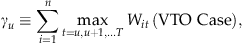
Finally, to model disruption costs associated with updated agent schedules, we include a cost c_d for each individual agent whose schedule is changed in the updating process. In addition, we define γ_u to be the number of agents whose schedules would be updated if results of the rescheduling model were implemented before period u, where where Y_it (W_it ) is as defined in section 3.4.1 (3.4.2). The total disruption cost associated with updating agent schedules before period u is denoted and is calculated as γ_u c_d .

3.5.2. Determining Whether or Not to Implement the Proposed Schedule Update. The total costs associated with a schedule update before period u is denoted Δ ^u , with . Our methodology implements the updated schedule before period u only if Δ ^u <0, which means that the net value (cost) of the updated schedule is positive (negative).

If Δ ^u ≥0, schedules are not updated before period u, the actual call volume x_u for period u is observed, and the process described in sections 3.3 and 3.4 above is repeated.

4. Empirical Testing of Intra‐Day Rescheduling Methodology

4.1. Numerical Experiments: Description and Input Parameters

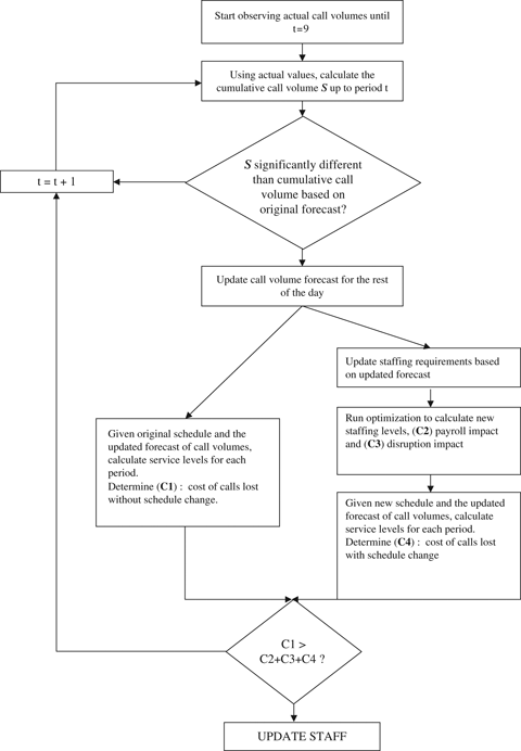
To test the rescheduling framework described in the previous section, we used data from an actual call center's operations to conduct a series of numerical experiments. For each day of operations, our experimental framework is illustrated in Figure 2. Our approach is to start with day‐of‐operations forecasts (“original forecasts”) and the associated agent schedules (“original schedules”). From here, we observe the actual call arrivals for each day and use this information to create “updated forecasts.” Next, we examine the updated forecasts in conjunction with the original schedules to determine if and when to update agent schedules. Finally, using the actual call arrivals for the entire day, we compare the performance of the call center when the original schedules are used for the entire day with the performance of the system when our rescheduling framework is used to update the schedules. This process is described in more detail below.

Figure 2

Rescheduling Framework and Experimental Workflow

4.1.1. Overview of Call Center and Determination of Original Schedules. The call center that was used for our numerical experiments was originally presented by Saltzman (2005). This call center provides support for an on‐line e‐commerce portal and is open from 6:00 am to 9:00 pm, with a schedule granularity of 15‐minute increments. The center employs 32‐types of agents, 10 with part‐time and 22 with full‐time schedules.

In order to calculate the initial target staffing levels d_t , we used day‐of‐operations forecasts for call arrival rates λ_t and average service rates μ_t . From here, the minimum number of agents required per period is calculated using the traditional stationary independent period by period (SIPP) transformation with a service‐level goal of answering 99% of calls within 300 seconds. Finally, the original agent schedules were created based on these day‐of‐operations forecasts and service‐level targets by using the schedule optimization algorithm from Saltzman (2005).

It is important to note that our day‐of‐operations forecasts λ_t can differ significantly from the 2‐week moving average forecasts actually used by this call center to determine agent requirements and create agent schedules. Specifically, we use the ratio of actual calls to forecasted calls during the first n days of the week to update the original forecast to get a day‐of‐operations forecast for the n+1st day. In addition, our original schedules are based on these day‐of‐operations forecasts, whereas the actual schedules for this call center were based only on the original forecasts.

4.1.2. Determining Whether or Not to Consider Updating Agent Schedules. The general process for determining when and how to update agent schedules is described in detail in sections 3.3–3.5. Below we provide additional details about the specific criteria used in our numerical experiments.

For each day in our experiments, the first allowable period for re‐scheduling is u=9, meaning that all of the estimates used for forecast updates are based on at least eight observations (that is, at least 2 hours of data). This is consistent with both current industry practice and with the empirical results of Shen and Huang (2008) about the performance of this forecast updating method, which suggests that accuracy increases greatly after the first few periods. Our last allowable period for re‐scheduling is u=17, meaning that the decision on whether or not to update call forecasts and agent schedules is based on at most 16 observations (that is, 4 hours of data).

For a given period u, we determine whether or not actual cumulative call arrivals are significantly higher (or lower) than forecasted cumulative call arrivals based on the value of π_u as described in section 3.3.2. In particular, in our experiments, we use the threshold value p ₁=0.2 (p ₂=0.8) to determine whether call volumes are significantly higher (lower) than expected, which in turn suggests that the system is potentially understaffed (overstaffed). Values of p ₁ and p ₂ closer to (or farther from) 0.5 correspond to a lower threshold (higher threshold) for concluding that the actual call arrivals have deviated significantly from the expected values.

4.1.3. Updating Forecasts and Agent Requirements. If we have determined that the call volumes are significantly higher or lower than expected, our next step is to make use of the call volumes observed in 1, 2, …, u−1 to update the demand for agents in period t for t=u, u+1, … , 60. This is done in two steps.

The first step is to create an updated forecast for the arrival rate in period t as of the beginning of period u, which we denote , where . The second step is to use the updated forecast in the standard SIPP procedure (as discussed in Green et al. 2001, 2003) to determine the updated agent requirements . The values of the incremental agent demand levels are then computed as the difference between and .

4.1.4. Creating Updated Agent Schedules and Evaluating the Associated Benefits. After determining the updated agent requirements and incremental agent demand levels, for understaffed cases (overstaffed cases) the integer program to update schedules from section 3.4.1 (section 3.4.2) is solved to determine the updated schedules. Once the updated schedules have been identified, we determine the net value of updating the schedules as of time u by following the procedure described in section 3.5, using the following cost parameters.

For our numerical experiments, we used a standard labor cost of US$20/hour for all agents of all types as in Saltzman (2005) as well as values of US$15/hour for the savings rate s_i associated with an hour of VTO for all agents and a value of US$27/hour for the overtime cost o_i for all agents who are already scheduled. In addition, we used a value of US$36/hour for the hourly cost for any previously unscheduled agents who are called in to meet the increased demand levels. In practice, call‐in agents are asked to show up whenever needed and on very short notice, which is the justification for the higher overtime costs. We assessed a cost of US$25/call for each call not answered within the service‐level target period. Finally, we included a charge of US$5 for each individual agent whose schedule was changed, and this disruption charge was explicitly included in our calculation of the net value of any given schedule update, as described in section 3.5.

4.2 Experimental Results

4.2.1. Initial Results. Our numerical experiments are based on weeks of day‐of‐operations forecasts and call arrival data, for a total of 32 distinct days of call center operations. Our presentation of numerical results is focused on the financial impact of the schedule updates. At the end of each day, we can estimate the financial impact of the schedule update decision by calculating the performance metrics using actual call volumes, first with the original agent schedules and then with the updated agent schedules.

For three of these 32 days, the model either did not identify any significant differences between the original call arrival forecast and the actual call arrivals or estimated that the value of updating agent schedules was less than the cost of disruption. Of the remaining 29 days, 16 were identified as “understaffed” and 13 were identified as “overstaffed.” For our initial tests, we used the updated value for the mean arrival rate to determine the updated agent requirements , as described in section 3.3.4.

When the early periods' call arrivals suggest that the call center is understaffed, our model seeks to increase staffing levels to meet service‐level goals and reduce lost calls for the remainder of the day. For days that were identified as understaffed, Table 1 illustrates the impact of the schedule updating model on these metrics. In particular, we note that schedule updating has a strong impact on the achieved service levels (with the mean increasing from 83.50% under the original schedules to 89.07% in the presence of updated schedules). As such, the cost of calls that fail to meet the service‐level objective decreases substantially as a result of our intra‐day rescheduling, in all cases exceeding the cost of additional staff and the cost of disruption.

Table 1

Summary Results for the Days Identified as Understaffed

Performance measure	“End‐of‐day” comparison based on actual call arrivals
Mean service level (%)
With the updated schedule	83.50
With the original schedule	89.07
Δ	5.57
Mean cost of not meeting SL targets (US$)
With the updated schedule	12,798
With the original schedule	19,112
Δ	−6,314
Payroll impact of update (US$)	3,902
Disruption impact of update (US$)	61

When the early periods' call arrivals suggest that the call center is overstaffed, our model seeks to reduce staffing levels, reducing labor costs and thereby increasing agent utilization levels, while also continuing to achieve the service‐level objectives. For days that were identified as overstaffed, Table 2 illustrates the impact of the schedule updating model. In the overstaffed case, we see that the cost of lost calls grows as a result of the decision to update agent schedules and that on average this cost exceeds the amount that is saved as a result of decreased labor costs. In addition, we notice that even the original schedules fail to meet the service‐level objectives over the course of the day; this reflects the fact that, for this call center, some days' actual call arrivals are greater than expected in later periods even though the early periods are lower than expected. We address this phenomenon with additional experiments, which are described in the next section.

Table 2

Summary Results for the Days Identified as Overstaffed

Performance measure	“End‐of‐day” comparison based on actual call arrivals
Service level (%)
With the updated schedule	81.33
With the original schedule	97.37
Δ	−16.04
Cost of not meeting SL targets (US$)
With the updated schedule	18,505
With the original schedule	2,693
Δ	15,812
Payroll impact of update (US$)	−2,015
Disruption impact of update (US$)	335

4.2.2. Incorporating Distributional Information in Determining Updated Agent Requirements. In our next round of numerical experiments, we explored the impact of using additional distributional information to determine the updated agent requirements , as described in section 3.3.4 above. In particular, in understaffed (overstaffed) situations, we define values k ₁>0 (k ₂>0) and then use as the updated mean arrival rates that are used to determine , where σ_t is the standard deviation of the call volume distribution for period t for t=u, u+1, … , 60.

The parameters k ₁ and k ₂ can be interpreted as “insurance” against the remaining arrival rate uncertainty, with larger k_i values corresponding to more conservative estimates of the updated arrival rate. In the understaffed case, a positive value of k ₁ corresponds to a more aggressive attempt to meet service levels in periods u, u+1, … , 60 by adding more staff hours during the re‐scheduling process than in our initial experiments, which correspond to the case where k ₁=0. Conversely, in the overstaffed case, a positive value of k ₂ corresponds to a more conservative approach to releasing resources that might be needed in the event of higher‐than‐expected call volumes in future periods than in our initial experiments, which correspond to the case where k ₂=0.

During the 16 days that were identified as understaffed, we ran experiments with values of k ₁ ranging from 0.25 to 2.5 with increments of 0.25. The results are shown in Table 3. While increased values of k ₁ always correspond to higher target values of and therefore lower costs associated with calls that fail to meet service level, it is interesting to note that the net benefit peaks when k ₁=1.25 For k ₁>1.25, the mean incremental benefits associated with improving service levels fell short of the cost of increased staff hours and disruption.

Table 3

Summary Results for the Days Identified as Understaffed with Different k ₁ Values

k ₁	SL w/o update (%)	SL w/update (%)	Cost of calls lost w/o update (US$)	Cost of calls lost w/update (US$)	Cost of update (US$)	Cost of disruption (US$)	Net benefit (US$)
0.25	83.50	91.34	19,112	10,189	4,678	72	4,172
0.50	83.50	92.32	19,112	9,066	5,374	77	4,595
0.75	83.50	93.36	19,112	7,865	6,131	89	5,027
1.00	83.50	94.43	19,112	6,643	6,926	97	5,445
1.25	83.50	95.53	19,112	5,313	7,752	104	5,943
1.50	83.50	96.30	19,112	4,417	8,600	108	5,987
1.75	83.50	96.68	19,112	3,980	9,466	112	5,554
2.00	83.50	97.07	19,112	3,512	10,320	118	5,161
2.25	83.50	97.61	19,112	2,862	11,199	125	4,926
2.50	83.50	97.72	19,112	2,710	12,080	125	4,197

On the other hand, the 13 days identified as overstaffed show somewhat different dynamics. In particular, the higher the value of k ₂, the smaller the change to staffing levels and the lower the loss associated with calls in future periods that do not achieve the service‐level goal (Table 4).

Table 4

Summary Results for the Days Identified as Overstaffed with Different k ₂ Values

k ₂	SL w/o update (%)	SL w/update (%)	Cost of calls lost w/o update (US$)	Cost of calls lost w/update (US$)	Cost of update (US$)	Cost of disruption (US$)	Net benefit (US$)
0.25	97.37	84.76	2,693.02	15,127.92	1,790.14	327.86	10,972.61
0.50	97.37	87.43	2,693.02	12,573.83	1,562.14	321.79	8,640.45
0.75	97.37	89.25	2,693.02	10,806.28	1,333.71	311.79	7,091.33
1.00	97.37	90.94	2,693.02	9,128.89	1,141.29	294.29	5,588.87
1.25	97.37	92.96	2,693.02	7,105.36	937.71	279.29	3,753.92
1.50	97.37	94.41	2,693.02	5,668.62	753.86	265.71	2,487.46
1.75	97.37	95.48	2,693.02	4,580.73	603.00	249.29	1,534.00
2.00	97.37	96.23	2,693.02	3,841.74	459.43	231.07	920.37
2.25	97.37	96.77	2,693.02	3,295.02	342.86	212.14	471.29
2.50	97.37	97.06	2,693.02	3,000.02	232.71	181.79	256.08

5. Conclusions and Next Steps for Research

In this paper, we have described an important business problem associated with real‐time schedule adjustments for call center operations. The methodology that we have developed here enables managers to update daily workload forecasts and demand for agent resources by leveraging information obtained from observations of call traffic early in the day, and to then use these updated demand levels to intelligently re‐schedule agents across a range of feasible adjustments. Our experimental results, based on data from an actual sales‐and‐service call center, show that there is significant business value associated with such intra‐day adjustments when the call center appears to be understaffed. When this particular call center appears to be overstaffed, on the other hand, there appears to be significant risk associated with releasing agents from their schedules, although our rescheduling framework provides an approach to mitigating this risk.

In developing our methodology, we have connected major ideas from the forecasting and forecast updating literature and from the optimal shift scheduling literature to produce an integrated solution for schedule updating. In addition, we have demonstrated the use of this methodology to update day‐of‐operations forecasts and agent schedules for an actual call center.

We believe that the area of intra‐day/real‐time schedule adjustments has received insufficient research attention, both in the call center literature and in the personnel scheduling literature overall. As such, we conclude by suggesting several other related research questions.

One obvious critical input to this process is the joint distribution of (and correlation between) calls during different intervals within the same day. While a few papers have appeared in the literature recently (Avramidis et al. 2004, Brown et al. 2005, Shen and Huang 2008, Weinberg et al. 2007), there is still a need for additional work in this area, as improved intra‐day forecast updates will lead to better intra‐day schedule updates.

A related issue is the process of determining of initial (and updated) staffing levels and the impact of these decisions on agent schedules. Historically, agent requirement calculations have been made under the assumption of a deterministic arrival rate (the so‐called SIPP method) and in turn agent schedules have been based on these agent requirement levels. Recent work by Steckley et al. (2009) proposes an approximation method for determining staffing requirements to achieve a certain service‐level objective while explicitly accounting for arrival rate variability. As such, another avenue for investigating real‐time schedule updates for call centers is to examine the effect of using such approximations for determining the agent requirement levels used to determine the initial agent schedules and/or updated agent schedules.

For understaffed situations, our model assumes that there are additional resources available on an on‐call basis that can be added to the schedule to help meet the higher‐than‐expected demand levels. In practice, such agents are often likely to be contracted by a third‐party, a relationship commonly referred to as “outsourcing.” Because of the rapid growth in the call center outsourcing industry, contracting and utilizing contingent resources has recently been explored by several researchers, including Milner and Lennon‐Olson (2008), Bhandari et al. (2008), and Gans and Zhou (2007). Exploring contract structures and contingent capacity planning models in the context of schedule updating, variable arrival rates, and cross‐period correlation is of both theoretical and practical interest.

Finally, there is clearly a need to extend this type of schedule updating framework to include more sophisticated and increasingly common call arrival and call management issues such as customer messages leading to callbacks (Armony and Maglaras 2004) and skill‐based routing (Harrison and Zeevi 2005, Pot and Koole 2005, and Wallace and Whitt 2005).

Footnotes

Appendix

Acknowledgments

We would like to thank the editor and the anonymous referees for the invaluable feedback they provided during the revision of this manuscript.

References

Abernathy

W. J.

Baloff

Hershey

J. C.

Wandel

. 1973. A three‐stage manpower planning and scheduling model—a service‐sector example. Oper. Res. 22 (3): 693–711.

Aksin

Armony

Mehrotra

. 2007. The modern call‐center: A multi-disciplinary perspective on operations management research. Prod. Oper. Manag. 16 (6): 665–688.

Andrews

B. H.

Cunningham

S. M.

. 1995. L.L. Bean improves call‐center forecasting. Interfaces 25 (6): 1–13.

Armony

Maglaras

. 2004. On customer contact centers with a call‐back option: Customer decisions, routing rules, and system design. Oper. Res. 52 (2): 271–292.

Avramidis

A. N.

Deslauriers

L'Ecuyer

. 2004. Modeling daily arrivals to a telephone call center. Manage. Sci. 50 (7): 896–908.

Bhandari

Harchol‐Balter Scheller‐Wolf

. 2008. An exact and efficient algorithm for the constrained dynamic operator staffing problem for call centers. Manage. Sci. 54 (2): 339–353.

Bodily

S. E.

Freeland

J. R.

. 1988. A simulation of techniques for forecasting shipments using firm orders‐to‐date. J. Oper. Res. Soc. 39 (9): 833–846.

Brown

L. D.

Gans

Mandelbaum

Sakov

Shen

Zeltyn

Zhao

. 2005. Statistical analysis of a telephone call center: A queueing-science perspective. J. Am. Stat. Assoc. 100 (469): 36–50.

Cleveland

Mayben

. 1997. Call Center Management on Fast Forward. Call Center Press, Annapolis, MD.

10.

Easton

F. F.

Goodale

. 2005. Schedule recovery: Unplanned absences in service operations. Decision Sci. 36 (3): 459–488.

11.

Ernst

A. T.

Jiang

Krishnamoorthy

Owens

Sier

. 2004. An annotated bibliography of personnel scheduling and rostering. Ann. Oper. Res. 127 (1–4): 21–144.

12.

Fylstra

Lasdon

Watson

Waren

. 1998. Design and use of the Microsoft Excel solver. Interfaces 28 (5): 29–55.

13.

Gans

Koole

Mandelbaum

. 2003. Telephone call centers: Tutorial, review and research prospects. Manuf. Serv. Oper. Manage. 5 (2): 79–141.

14.

Gans

Zhou

Y.‐P.

. 2007. Call‐routing schemes for call‐center outsourcing. Manuf. Serv. Oper. Manage. 9 (1): 33–50.

15.

Grassman

W. K.

1988. Finding the right number of servers in real‐world queueing systems. Interfaces 18 (2): 94–104.

16.

Green

L. V.

Kolesar

P. J.

Soares

. 2001. Improving the SIPP approach for staffing service systems that have cyclic demands. Oper. Res. 49 (4): 549–564.

17.

Green

L. V.

Kolesar

P. J.

Soares

. 2003. An improved heuristic for staffing telephone call centers with limited operating hours. Prod. Oper. Manag. 12 (1): 1–16.

18.

Guerrero

V. M.

Elizondo

J. A.

. 1997. Forecasting a cumulative variable based on its partially accumulated data. Manage. Sci. 43 (6): 879–889.

19.

Harrison

J. M.

Zeevi

. 2005. A method for staffing large call centers using stochastic fluid models. Manuf. Serv. Oper. Manage. 7 (1): 20–36.

20.

Hur

2002. A comparative evaluation of forecast monitoring systems in service organizations. 33rd Annual Meeting of the Decision Sciences Institute, San Diego, CA.

21.

Hur

Mabert

V. A.

Bretthauer

K. M.

. 2004. Real‐time work schedule adjustment decisions: An investigation and evaluation. Prod. Oper. Manag. 13 (4): 322–339.

22.

Jongbloed

Koole

. 2001. Managing uncertainty in call centers using Poisson mixtures. Appl. Stoch. Models Bus. Ind. 17 (2001): 307–318.

23.

Kekre

Morton

T. E.

Smunt

T. L.

. 1990. Forecasting using partially known demands. Int. J. Forecast. 6 (1): 115–125.

24.

Mabert

V. A.

1991. Ohio Valley National Bank, Cases in Manufacturing and Services Management. Prentice Hall, Englewood Cliffs, NJ.

25.

Mabert

V. A.

1995. PSI Energy's call center. Unpublished case study, Indiana University, IN.

26.

Mehrotra

1997. Ringing up big business. OR/MS Today 24 (4): 18–24.

27.

Mehrotra

Wright

Patel

. 2009. An investigation into the business processes, job descriptions, and human resource factors associated with successful workforce management practice, Working Paper, San Francisco State University, San Francisco, CA.

28.

Milner

Lennon‐Olson

. 2008. Service level agreements in call centers: Perils and prescriptions. Manage. Sci. 54 (2): 238–252.

29.

Pot

Koole

. 2005. Approximate dynamic programming for multi‐skill call centers. Proceedings of the 2005 Winter Simulation Conference, Piscataway, NJ.

30.

Robbins

T. R.

2007. Addressing Arrival Rate Uncertainty in Call Center Workforce Management. Proceedings of the 2007 IEEE/INFORMS International Conference on Service Operations and Logistics, and Informatics, Philadelphia, PA.

31.

Saltzman

2005. A hybrid approach to minimizing the cost of staffing a call center. Int. J. Oper. Quant. Manage. 11 (1): 1–14.

32.

Shen

Huang

J. Z.

. 2008. Interday forecasting and Intraday updating of call center arrivals. Manuf. Serv. Oper. Manage. 10 (3): 391–410.

33.

Steckley

Henderson

Mehrotra

. 2004. Service system planning in the presence of a random arrival rate. Working paper, Department of Operations Research and Industrial Engineering, Cornell University, Ithaca, NY.

34.

Steckley

Henderson

Mehrotra

. 2009. Forecast errors in service systems. Probab. Eng. Inf. Sci. 23 (2): 305–332.

35.

Thompson

G. M.

1996. Controlling actions in daily workforce schedules. Cornell Hotel Restaurant Admin. Q. 37 (2): 82–96.

36.

Thompson

G. M.

1998. Labor scheduling, part 1: Forecasting demand. Cornell Hotel Restaurant Admin. Q. 39 (5): 22–31.

37.

Thompson

G. M.

1999. Labor scheduling, part 4: Controlling workforce schedules in real-time. Cornell Hotel Restaurant Admin. Q. 40 (3): 85–96.

38.

Wallace

Whitt

. 2005. A staffing algorithm for call centers with skill‐based routing. Manuf. Serv. Oper. Manage. 7 (4): 276–294.

39.

Weinberg

Brown

J. L. D.

Stroud

J. R.

. 2007. Bayesian forecasting of an inhomogeneous Poisson process with applications to call center data. J. Am. Stat. Assoc. 102 (480): 1185–1198.

40.

Whitt

1999. Dynamic staffing in a telephone call center aiming to immediately answer all calls. Oper. Res. Lett. 24 (5): 205–212.

41.

Whitt

2002. Stochastic‐Process Limits. Springer Series in Operations Research. Springer, New York.

42.

Whitt

2006. Staffing a call center with uncertain arrival rate and absenteeism. Prod. Oper. Manag. 15 (1): 88–102.