
Abstract
This paper investigates the effect of learning and forgetting on production scheduling decisions. Numerous papers have appeared on this topic in the last four decades; they show that firms are better off producing in larger batches in the presence of learning and forgetting. However, these papers fail to consider one or more of realistic features of learning and forgetting; factors such as (1) the amount forgotten increases with break length between two batches and (2) the forgetting could be slow over an initial short interval followed by fast forgetting. Our paper contributes by demonstrating that a consideration of these realistic features leads to a different conclusion—firms may be better off producing in smaller batches in the presence of learning and forgetting. This is a new insight that provides one more justification for producing in small batches.
1. Introduction
This paper investigates the effect of learning and forgetting on production batch sizes by considering a single‐product manufacturing environment where production takes place in batches. Because of batching, workers go through learn, forget, and re‐learn cycles. Learning in production time occurs while producing units in a batch, forgetting during the break between two batches, and re‐learning when production resumes after the break.
The issue of the effect of learning and forgetting on productivity is an important one; see, for example, Argote and Epple (1990), who noted: “Large increases in productivity are typically realized as organizations gain experience in production. These learning curves have been found in many organizations. Organizations vary considerably in the rates at which they learn. Some organizations show remarkable productivity gains, whereas others show little or no learning. Reasons for the variation observed in organizational learning curves include forgetting, employee turnover, transfer of knowledge from other products, and other organizations and economies of scale.” They suggest that considering forgetting and other factors that affect productivity gains should enable managers to make better production scheduling decisions. Learning and forgetting have gained attention from several other scholars over the last decade. Lanier (2000) found that learning alone was not sufficient to explain labor requirements for Lockheed L‐1011 (commercial aircraft) production. Argote et al. (1990) conducted an empirical study on the persistence and transfer of organizational learning. A recent paper by Holan et al. (2004) addressed the importance of managing the organizational forgetting.
Beginning from Keachie and Fontana (1966), many papers have considered the effect of learning and forgetting on production scheduling decisions. These papers differ from each other in the assumptions on how forgetting occurs and whether the demand rate is constant or dynamic. Most of these papers use Wright's (1936) learning function. Keachie and Fontana (1966) applied learning and forgetting to the Economic Order Quantity (EOQ) model with equal lot‐size restriction under the assumption that the amount of forgetting depends on the cumulative number of interruptions so far. Under the assumption that there is complete transfer of learning from batch to batch, Steedman (1970) showed that the optimal lot size in Keachie and Fontana's model is larger than that in the traditional EOQ model. Spradlin and Pierce (1967) relaxed the equal lot‐size assumption. In their forgetting model, they assumed that the amount of the regression in learning due to an interruption in production is equal to the amount learned during the production of the last M units. Fisk and Ballou (1982) extended the work in Spradlin and Pierce (1967) by assuming that the inventory level increases non‐linearly over the production interval. Smunt and Morton (1985) modified Fisk and Ballou's (1982) model by assuming the holding cost to be a function of the production cost for the lot. Both Fisk and Ballou (1982) and Smunt and Morton (1985) use the same forgetting function, which assumes that the forgetting between batches occurs as a fixed portion of the previous experience. Both papers concluded that the effect of forgetting is to increase the batch size. Sule (1978), Axsater and Elmaghraby (1981), and Elmaghraby (1990) studied the convergence of production time under the constant demand and the constant lot‐size assumption. They allowed the amount forgotten during an interruption to depend on the length of the interruption, but their forgetting function made some unrealistic assumptions as discussed in the next section of this paper. Li and Chen (1994) considered the lot‐sizing problem with learning in setups and learning and forgetting in production. Their forgetting model, similar to the one in Smunt and Morton (1985), assumes that the amount forgotten is equal to a fixed portion of the total learning so far. Chiu (1997) considered the problem when demand is time‐varying. He also concluded that, in a fast forgetting environment, the optimal lot size is larger than that in a slow forgetting environment. Chiu et al. (2003) investigated the similar problem under the presence of learning and forgetting in both setup and production. They assumed that the amount forgotten depends on the length of interruption but cannot exceed the amount learnt in the previous batch. The focus in their paper was on algorithmic efficiency and not on studying the effect of learning and forgetting on batch sizes.
From our literature review, we found that a key weakness of a number of papers that consider the effect of learning and forgetting on batch sizes is the assumption that the amount forgotten is independent of the length of interruption. According to Bailey (1989), there is evidence in the Psychology literature that forgetting is a function of the amount learnt so far and the length of interruption. Globerson et al. (1998) provides data and mathematical models on the effect of length of interruption on forgetting. Dar‐El (2000) provides a comprehensive review of factors that influence forgetting. The papers on batch sizing that allow forgetting to depend on the length of interruption use forgetting functions that do not satisfy one or more of realistic characteristics of forgetting—characteristics such as you can only forget what you have learnt so far, and no more. We will refer to these as “basic characteristics” in the rest of this paper.
This paper contributes by providing a rigorous treatment to a problem that has been considered by a number of researchers in the literature. We use forgetting functions that are more realistic. We allow delayed forgetting; that is, there could be slow forgetting over an initial short interval followed by fast forgetting. Our computational results show that there are situations when the effect of forgetting is to reduce batch sizes. To the best of our knowledge, this is the first paper that shows that the manager may be better off producing in smaller batches in the presence of forgetting. Thus, our results provide one more justification for the practice of producing in small batches in just‐in‐time (JIT) manufacturing. This paper also shows that the cost of ignoring learning and forgetting can be high.
Section 2 of this paper briefly reviews learning and forgetting models in the literature and justifies the models we use. A more complete review of learning and forgetting models is provided in Appendix A. Section 3 formulates the lot‐sizing problem with learning and forgetting. It also presents a forward recursive algorithm to find an optimal production plan. Section 4 provides computational results and managerial insights. This paper closes in section 5 by providing concluding remarks.
2. Learning and Forgetting Models
We first review Wright's learning function and justify its use in our research. We then present some basic properties that forgetting functions should satisfy. We review a number of forgetting models in the literature and justify the models we use.
2.1. Wright's Learning Model
We use Wright's model, which suggests that when the cumulative number of units produced doubles, the unit production time decreases by a constant percentage. Yelle (1979) provided a thorough review of the learning curve literature. Dar‐El et al. (1995) indicated that Wright's learning curve is widely used in practice because of its simplicity and sufficient ability to predict. Globerson (1980) conducted a laboratory study to investigate the predictability power of three different learning curves. He concluded that Wright's power learning curve is the best predictor. We next provide specifications for Wright's learning function.
Let T(x) be the unit production time of the xth unit and let 100(1−p) be the percentage decline in the unit production time with doubling of units produced, then 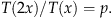
Defining m=−log(p)/log(2) so that 2−m=p, we obtain 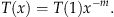
Note that m=0 implies T(x)=T(1) for all values of x, and therefore there is no learning. Large m (or small p) implies faster learning. We next discuss the forgetting phenomenon.
2.2. Review of Forgetting Models
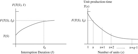
Assume that the experience level at the current time is such that the time to produce one unit would be X if the worker were to start producing immediately. There is an interruption of I periods and we are interested in finding the unit production time at the end of the interruption. If there were no forgetting, then the time for the unit would be X. However, the time will be larger than X with forgetting. If we let F(X, I) denote the unit production time for the unit after interruption of I periods, then F(X, I)≥X, and F(X, I)−X is the amount forgotten. The purpose of forgetting functions is to provide an expression or a procedure to compute F(X, I). Note that (T(1)−X) is the amount learnt so far—a measure of the experience level.
In our study, we desire forgetting functions that satisfy the following basic properties.
F(X, I+Δ)>F(X, I) for Δ>0. (F(X, I)−X) is increasing in (T(1)−X).
 .
.
Properties (1) and (2) are reasonable approximations for most manufacturing environments. Together, these properties imply that the amount forgotten is increasing in I and that it approaches T(1)−X (the amount that has been learnt so far) as I approaches ∞. Property (3) says that more is forgotten if there is more to forget. A justification for properties (2) and (3) comes from Bailey (1989) and Shtub et al. (1993), who noted that the amount forgotten during an interruption is a function of the amount learnt so far and the length of the interruption.
Both exponential and S‐shaped forgetting functions introduced by Globerson and Levin (1987) satisfy all of the basic properties. Most other forgetting models proposed in the literature do not satisfy one or more of the basic properties. For example, forgetting is not a function of the break length in Keachie and Fontana (1966), Spradlin and Pierce (1967), Fisk and Ballou (1982), Smunt (1987), and Chiu (1997). Carlson and Rowe's (1976) and Sule's (1978) power forgetting functions allow the amount forgotten to exceed the amount learnt; that is, as the break length increases, time for the unit after the break becomes large without any bound. Globerson et al. (1989) propose another power forgetting function, but it has the same limitation as Carlson and Rowe (1976). In Chiu et al. (2003), the amount forgotten depends on the break length but cannot exceed the amount learnt in the previous batch.
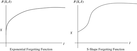
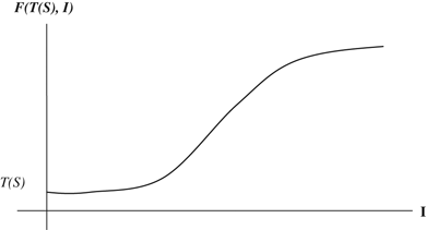
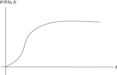
Based on the above considerations, we chose exponential and S‐shaped forgetting functions. Nembhard and Osothsilp (2001) provided empirical evidence for these. The exponential forgetting function assumes that there is a rapid initial decrease in performance followed by a gradual leveling off. The S‐shaped forgetting function assumes that there is slow forgetting over an initial short period, followed by a period of rapid forgetting, and then gradual leveling off (see Figure 1).
We next present these functions. The parameter b>0 is the “forgetting coefficient.” Recall that F(X, I) is the unit production time after a break of I periods.
Exponential forgetting function:

S‐shaped forgetting function:

In both functions, the larger the b, the greater is F(X, I)−X, or the amount forgotten. For example, for b=∞, F(X, I)=T(1), and there is complete forgetting for any I. (A summary of several other important learning and forgetting models is provided in Appendix A.)
2.3. Production Time for a Batch of q Units
Assume that we just finished a unit, the production time for the unit was T(S−1), and we are interested in finding the production time for a batch of q units if the production were to start after a break of I
0 periods. As done in the literature, we assume that the worker will start on the original learning curve at an experience level that corresponds to unit production time after the interruption, and then move down the learning curve in the production of q units. (This assumption originates from the early works of Carlson and Rowe 1976, Sule 1978, and Elmaghraby 1990.) Note that, following Wright's learning curve, the production time for next unit is T(S) if there is no interruption. Let α be such that F(T(S), I
0)=T(1)α
−
m
, then we obtain 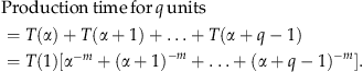
See Figure 2 for an illustration of forgetting and re‐learning cycles.
The next section specifies the model assumptions for the environment we consider, and develops a forward recursive algorithm to find optimal decisions. This recursive algorithm is essentially an efficient procedure for complete enumeration.
3. Model Formulation and a Forward Recursive Algorithm
We start with model assumptions. We then explain calculations of start and completion times for batches in a production plan and its cost. Finally, we present a forward recursive algorithm and discuss its computational requirements.
3.1. Model Assumptions
We consider a finite‐horizon problem consisting of periods 1, 2, …, T, with known demands d 1, d 2, …, dT in these periods, and where the objective is to select production batch sizes that meet all demands at the minimum possible cost. The model makes the following major assumptions for the manufacturing environment that we consider.
A
A
The first assumption is a standard assumption in MRP‐type environments where units for the entire demand in a period should be available at the beginning of the period. Assumption II prohibits allocating the demand in a period to two or more batches produced at different times. This is a reasonable assumption because producing a given demand in different batches will increase the difficulty of coordination. Assumption II also implies that the first dt units in a batch are produced just in time to meet the demand in t, which is also a reasonable assumption for practical problems.
3.2. Start and Completion Times
A production plan that consists of n batches (n≤T) can be specified by n numbers t 1=1<t 2<t 3< … <tn ≤T, such that the ith batch (i=1, 2, …, n−1) covers the demands in periods ti to t i+1−1 and the nth batch covers the demands in periods tn to T. The start and completion times of the batches can be found using the learning and forgetting models and Assumption II regarding the start time of a batch. In addition, we can find the start and completion times of every unit in a batch (we need these for calculating holding costs). These times are unique for given batch sizes (see Result 1).
Start and completion times for batches in a given production plan are feasible if production intervals for two consecutive batches do not overlap. We make an assumption to guarantee that such an overlap will not occur. To state this assumption we define “production capacity in a period” as the number of units that can be produced in the period starting from zero experience at the beginning of the period.
A
We make this assumption to keep the presentation simple. The assumption is not restrictive for the insights we are trying to develop in this paper. We next give a numerical example to illustrate computations of start and completion times.
E
From 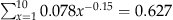 , the first batch needs to start 0.627 time units before beginning of period 1 so that d
1=10 units will complete at the beginning of period 1. For the second batch, we need to choose the start time for d
2 so that d
2 units will complete at the beginning of period 2. The production time for d
2 determines the length of interruption (I=1−Production Time for d
2). However, the length of interruption determines the experience level at the start of (production of) d
2, and therefore the production time for d
2. We had to resort to a numerical procedure (bi‐section method) to compute the length of interruption; it was not possible to find a closed‐form expression.
, the first batch needs to start 0.627 time units before beginning of period 1 so that d
1=10 units will complete at the beginning of period 1. For the second batch, we need to choose the start time for d
2 so that d
2 units will complete at the beginning of period 2. The production time for d
2 determines the length of interruption (I=1−Production Time for d
2). However, the length of interruption determines the experience level at the start of (production of) d
2, and therefore the production time for d
2. We had to resort to a numerical procedure (bi‐section method) to compute the length of interruption; it was not possible to find a closed‐form expression.
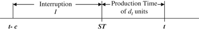
For our numerical procedure to work, we need to prove that the start time is unique. Consider the situation in Figure 3; t−c denotes the completion time of the previous batch and ST denotes the start time for dt units.
R
P
We now provide a brief description of the bi‐section method. We let PT(I) denote the production time for the batch.
3.3. Bi‐Section Method
The purpose is to find the root of the equation f(I)=I+PT(I)−c=0. We start with two guesses for I, a high value H where the function is positive and a low value L where the function is negative. We divide the interval from L to H into two halves, and select the half that contains the root. (If the function is positive at the mid‐point, then the first half of the interval contains the root, otherwise the second half contains the root.) We repeat this process until the interval becomes sufficiently small.
Using our numerical procedure, we obtain Interruption Duration=0.524, Experience Level at the start of d 2=3.22, and Production Time for d 2=0.475.
3.4. Cost of a Plan
The cost of a plan includes the setup cost, the direct labor cost, and the holding cost. To calculate the setup cost, we assume that there is a fixed cost of US$K for every batch. The direct labor cost for a batch is assumed to be w times the production time for the batch. We assume a holding cost of US$h per unit per period for the completed units in inventory. We know the completion time and the usage time (or the time when the unit is used to meet demand) for every unit in the plan, and therefore we know the flow time (or the amount of time the unit spends in inventory after completion) for every unit in the plan. The holding cost for a unit can be found simply by multiplying the unit's flow time with h. We next develop a forward recursive algorithm to find an optimal production plan under model Assumptions I–III.
3.5. A Forward Recursive Algorithm
Define C(t) as the minimum cost of meeting demands in periods 1 to t with zero initial inventory and zero inventory at the end of period t. Assume C(0)=0. We need a notation for a schedule for periods 1 to t. We let Zt
be a set of integers {t
1=1, t
2, t
3, …, tn
≤t} that specify a production schedule with n batches for the first t periods. (We assume d
1>0, and therefore t
1 is always equal to 1.) We let {Zt
} denote the set of all possible production schedules for t periods. It is easy to see that there are 2
t−1 schedules in {Zt
}, and the number of batches (n) ranges from 1 to t. Also, we let  denote the cost of a Zt
‐schedule. We define Z
0 to be an empty set with
denote the cost of a Zt
‐schedule. We define Z
0 to be an empty set with  . We have
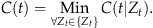
In our forward algorithm, we do calculations for the (t−1)‐period problem before going to t. Two questions need to be answered: (i) when going from t−1 to t, how do we generate all {Zt
} schedules and (ii) how do we efficiently calculate  for these schedules? It is easy to see that
If Zt
=Z
j−1∪{j} for some j, then  can be calculated as follows:
 is the cost to cover the demands in the first j−1 periods using schedule Z
j−1 and
is the cost to cover the demands in the first j−1 periods using schedule Z
j−1 and  is the cost for the last production batch that covers the demands in periods j to t given that Z
j−1 covers the demands in the first j−1 periods. Note that, for the first j−1 periods, we need the cost
is the cost for the last production batch that covers the demands in periods j to t given that Z
j−1 covers the demands in the first j−1 periods. Note that, for the first j−1 periods, we need the cost  , and not just C(j−1), because the experience associated with the schedule Z
j−1 affects the production cost in periods j to t.
, and not just C(j−1), because the experience associated with the schedule Z
j−1 affects the production cost in periods j to t.
Details for calculating  are provided in Appendix B. We need Assumption III to guarantee a feasible solution for
  . Our algorithm generates 2
k−1 schedules in going from period k−1 to period k and performs O(dk
) calculations to compute the holding cost for each of these schedules. Thus, our forward program requires
. Our algorithm generates 2
k−1 schedules in going from period k−1 to period k and performs O(dk
) calculations to compute the holding cost for each of these schedules. Thus, our forward program requires 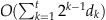 calculations to solve the t‐period problem. Our algorithm is exponential in time and pseudo‐polynomial in the demand data.
While the computational complexity of our algorithm is comparable to that of a complete search of the 2 k−1 schedules for a k‐period problem, our algorithm improves computational efficiency by using information for partial schedules in calculating the costs for longer schedules. In other words, the cost for a partial schedule that is part of several different longer schedules is calculated only once.
The next section provides a computational study to develop managerial insights.
4. Managerial Insights
This section first develops insights on the effect of learning and forgetting on batch sizes for a number of different problem parameters. We then present insights on the cost of ignoring learning and forgetting. We also discuss an alternative model for re‐learning and its impact on the managerial insights.
4.1. Effect of Learning and Forgetting on Batch Sizes
We used Constant, Increasing, Decreasing, and Seasonal demand patterns with parameter values shown below:
Constant Mean: dt
=μ+σzt
; μ=40 and σ=0, 7, 15, Increasing: dt
=μ+σzt
+r(t−1); μ=40, σ=0, 7, r=1, 1.5, and T=12, Decreasing: dt
=μ+σzt
+r(T−t); μ=40, σ=0, 7, r=1, 1.5, and T=12, Seasonal:
 ; μ=40, σ=0, 7, v=10, 20, and c=8, 12,
where dt is the demand in period t, zt is the standard normal variable, σ is the standard deviation, r is the additive trend factor, v is the amplitude of the seasonal component, and c represents the length of seasonal cycle in periods. In total, we have 19 demand patterns (see Table C1), each with the horizon length (T) of 12. Note that for increasing and decreasing demand patterns, as well as the seasonal demand, we used the approach in Fisher et al. (2001).
We solved each of these 19 problems for 24 different values of parameters in the learning and forgetting curves. We use three different learning rates (70%, 80%, and 90%), two different forgetting functions (exponential and S‐shaped), and four different values of the forgetting parameter b (3 for fast forgetting, 1 for moderate forgetting, 0.25 for slow forgetting, and 0.0 for no forgetting). We used a fixed production time T(1) of 0.0125 periods for the first unit. Altogether, there are 456 problems. The cost parameters are setup cost (K)=US$100.00 per setup, holding cost (h)=US$3.00 per unit per period, and wage rate (w)=US$100.00 per period. We used a Macro‐Visual‐Basic program to run the computations on a PC. Optimal solutions to these problems were found using our forward algorithm under model Assumptions I–III. (See Table D1 for a summary of the number of setups corresponding to the learning and forgetting parameters.)
We present four different insights that we obtained from our computational runs. Insight 1 is for slow‐forgetting S‐shaped functions. The benchmark solutions for this insight are the solutions with just learning and no forgetting.
Insight 1: There are instances when the number of batches increases in the presence of forgetting characterized by a slow‐forgetting S‐shaped function.
This result is explained by the fact that for a slow‐forgetting S‐shaped function, the rapid forgetting rate is delayed by a short interval. (Figure 4 shows the rapid forgetting rate beyond a short interval.) By producing at short intervals in small lots, we are able to gain the benefits of learning without incurring the cost of rapid forgetting. Both the production cost and the holding cost for such a schedule are low. We believe that slow‐forgetting S‐shaped functions are realistic. Evidence for this is provided in Nembhard and Osothsilp (2001). Although this insight is not surprising for the type of forgetting function we use, we are able to develop this because our model takes into account the dependency of loss of learning on the length of interruption and other features of realistic forgetting curves. This result contrasts the conclusion in the literature that a consequence of considering forgetting in batch sizing models is to reduce the number of batches (Jaber and Bonney 1996, Smunt 1987). These studies missed this important insight because they did not consider slow‐forgetting S‐shaped functions. This insight is quite interesting because it provides one more justification for the small‐lot production approach in JIT manufacturing environments. Our result also suggests that learning/forgetting, in addition to congestion effects (Karmarkar 1987) and quality effects (Porteus 1986), should be taken into account in determination of batch sizes.
The next insight is for exponential forgetting functions.
Insight 2: For an exponential forgetting function, as the level of forgetting increases (fast forgetting), the number of batches decreases.
This insight can be explained by the fact that, for an exponential forgetting function, the amount forgotten is large even for a short interruption (see Exponential Forgetting Function in Figure 1). When there is an interruption in production, even a short one, the production cost for the batch following the interruption goes up due to forgetting. This increase in the production cost due to an interruption can be viewed as a setup cost. Faster forgetting means a larger increase in the production cost and, therefore, a higher setup cost. We know from the inventory lot‐sizing literature that the effect of higher setup costs is to reduce the number of setups or the number of batches.
The next insight is for a fast‐forgetting S‐shaped forgetting function.
Insight 3: For a fast‐forgetting S‐shaped function, as the level of forgetting increases (fast forgetting), the number of batches decreases.
A fast‐forgetting S‐shaped function is similar to the exponential function because the forgetting rate is slow over only a very short interval, and therefore the explanation for this insight is the same as for Insight 2 (see Figure 5 for an illustration.)
An implication of Insights 2 and 3 is that producing in small lots is not cost effective in environments where forgetting rate is high. The next insight discusses the effect of learning.
Insight 4: For any given level of forgetting, as the ability to learn increases (fast learning), the number of batches increases.
In a fast learning environment, the increase in production cost due to an interruption is not too high because, although the worker loses some experience during the interruption, he/she can re‐learn fast. The influence of fast learning is to mitigate the effect of forgetting. Fast learning reduces the “setup cost effect” of forgetting, and therefore the number of batches goes up. An implication of this insight is that any investment that management makes in improving the ability of workers to learn faster can pay off in a small‐lot manufacturing environment.
We used different demand patterns to capture the effect of learning and forgetting. The results were the same for all patterns. Thus, we do not present results specific to different patterns.
To use the insights in the paper, a question that managers would need to address is how to estimate the type of forgetting (slow forgetting or fast forgetting) for the tasks in their respective manufacturing environments? Several authors have reported (see, e.g., Bailey 1989, Globerson et al. 1998) that the nature of tasks has an impact on the rate of forgetting. Bailey (1989) argued that “procedural” tasks should be distinguished from “continuous control” tasks. Bailey (1989) explains: “Procedural tasks consist of a series of discrete motor responses, such as pressing appropriate buttons or mounting appropriate disks to run a computer. Continuous control tasks involve repetitious movements, without a clear beginning or end, as with riding a bicycle or visually inspecting parts on an assembly line. Thus a procedural task consists more of deciding what to do than of learning the motion itself.” Bailey reported that forgetting rate is higher for procedural tasks than for continuous control tasks. Globerson et al. (1998) labeled the procedural tasks as “cognitive” and the continuous control tasks as “motor,” and reported similar findings. To summarize, managers should expect a higher rate of forgetting for tasks with high cognitive content. This also implies that, if an S‐shaped forgetting function is used, then the length of the initial interval over which the forgetting rate is slow is shorter for tasks with high cognitive content.
We next study the increase in cost if learning and forgetting are ignored.
4.2. Cost of Ignoring Learning and Forgetting
We conducted this computational study to investigate the potential cost of ignoring learning and forgetting for problems with the realistic learning and forgetting parameters. We found that the cost of ignoring learning and forgetting could be substantial.
Industrial learning rates have been addressed by several authors (Cole 1958, Hirsch 1952, etc.). Hirsch studied learning curves in building seven different machines by a single manufacturer. Hirsch concluded that the learning rate varied between 75.2% and 83.5%. Cole conducted a survey of non‐aircraft companies and found the learning rate varied between 77% and 82%.
Nembhard and Osothsilp (2001) conducted an empirical comparison of several forgetting models, including the exponential and S‐shaped forgetting models used in our study. Upon the request of the author, David Nembhard provided us the forgetting parameters. The forgetting parameter for both models is approximately 0.15.
To examine the potential cost of ignoring forgetting, we used the learning rate of 80% and forgetting parameter of 0.15. Other problem parameters are T(1)=0.025 periods, setup cost=US$200 per setup, holding cost=US$3 per unit per period, the wage rate=US$250 for the first unit, the problem horizon=12 periods, and the demand rate=40 units per period. When learning and forgetting are considered, the associated cost, C(12), is US$30,716.19. If the learning and forgetting are ignored, the associated cost, C(12), is US$36,766.58. Thus, the cost of ignoring learning and forgetting (using the industrial learning rate and forgetting parameter) is 19.70% of the minimum cost. This example shows that, in reality, the cost of ignoring learning and forgetting could be substantial.
4.3. Alternative Models for Re‐Learning Curve
There are a few recent publications (Bailey 1989, Globerson et al. 1998, Shtub, Levin, and Globerson 1993) that suggest a power graph for the new learning curve (after the break) that merges with the original learning curve after some cycles. This power graph has steeper slope than the original learning curve until it merges with the original curve (see, e.g., Figure 1 in Globerson et al. 1998).
Our new insight is that the batch sizes could reduce when there is slow forgetting over an initial interval. The advantage of small batch sizes is that there are short breaks in production runs and we stay close to the original learning, and thus avoid the cost of forgetting associated with large breaks that go with large batches. The cost of forgetting is an increasing function of the length of break no matter which re‐learning curve we use (see, e.g., Figure 2 in Shtub, Levin, and Globerson 1993). Thus, this insight is not affected by the new re‐learning curve. It is easy to justify that the other insights also hold.
We close our study by providing some concluding remarks.
5. Concluding Remarks
This paper has considered the production batch sizing problem with learning and forgetting in production times. A unique feature of our model is that we use forgetting functions that satisfy all the basic properties of forgetting. Specifically, forgetting functions used in our study allow forgetting to depend on the length of interruption and the experience level before an interruption, but do not allow the amount forgotten to exceed the amount learnt. We also allow slow forgetting over an initial interval. We develop a forward algorithm to solve the problem.
We use our algorithm to solve 456 problems to develop insights in to the effect of learning and forgetting on batch sizes. We find that forgetting has a “setup cost effect,” and when significant forgetting occurs over short interruptions, the number of batches goes down. However, in one important case we find that the number of batches could actually go up and the batch sizes on average could go down. This is the case where very slow forgetting occurs in the initial periods of an interruption, followed by fast forgetting in later periods (S‐shaped forgetting function). This type of forgetting is realistic for many practical situations. The effect of producing in small batch sizes at short intervals is that forgetting does not take effect or is minimal. Thus, our analysis provides one more justification for small‐lot production in JIT manufacturing environments. This insight we believe is a new insight.
Our paper has used a single‐item model to investigate the effect of learning and forgetting on batch sizes. A useful extension of the model will be to consider the problem with multiple products. As a result, the worker may be producing some other item over the interruption interval for an item. The rate of forgetting over the interruption interval may depend on what other item is being produced. In some cases, depending on how similar the items are, even learning may take place over the interruption.
A reviewer pointed out that there may be cases when the amount of forgetting for an interruption is low if the experience level of the firm is very high. This is opposite of property (3) in section 2. We agree that this may be true for some tasks, and intend to develop new forgetting models to accommodate this feature in our future research. However, it should be pointed out that firms with frequent interruptions in production are unlikely to reach the state with very high learning, and therefore the insights in this paper hold.