
Abstract
This paper builds a dynamic programming model to optimize the collections process in consumer credit. It determines which collections actions should be undertaken and how long they should be performed, including theoretical results about the form of the optimal policy under certain conditions. Finally, a case study is described based on data from the collections department of a European bank.
1. Introduction
Consumer credit modeling has received far less attention by researchers than corporate credit modeling. In particular, there has been no modeling undertaken in order to improve the management of the operations involved in recovering some or all of the debt incurred when a borrower defaults. Yet the US subprime mortgage crisis and its knock‐on effects has made bankers and ordinary citizens realize how important consumer credit is and the impact the resultant consumer defaults are having on the banking system and the whole economy. So there is an urgent need to improve the modeling of the recoveries and collection process in consumer credit. This is particularly the case for unsecured credit, because the collections process for secured credit can be modeled as a two‐stage process—what is the chance the lender will have to take possession of the security and how much will the lender get for the security.
This paper seeks to model the collections process of unsecured consumer credit debt. The collections department of the lender has a number of actions it can take to secure some repayment of the debt. These can range from telephone calls, gentle reminder letters, more formal letters, to getting agreement to reschedule repayment patterns. If these actions fail, the collectors occasionally can make home visits but more generally seek legal redress involving court proceedings and the use of bailiffs. The questions are which actions should be taken and how long should a particular course of action be undertaken before trying another action. These problems can be modeled in two different ways. In the first approach, the decisions are made each period in the light of the individual debtor's repayment performance up to that point. These models would give an adaptive collections policy that is optimal for each individual debtor. However, this means the resources required for collecting from an individual debtor will vary depending on random events in the repayment process. Evaluating the total resources needed to collect from a group of such debtors would require simulations of these random processes. In the second approach, the decision of which action to perform next and how long to undertake that action depends only on the debtor's total repayment up to that point and assumes an “average” recovery profile for each future action which depends only on this total repayment. This approach has the advantage that you can easily calculate what are the optimal actions that will be applied to the “average” debtor and what is the average cash flow of recoveries that will follow from these actions. These are exactly the forecasts those who have to manage a collections process need to make prospectively when they are deciding the resources needed in the collections department and reporting to those who have to deal with provisioning (setting aside money to cover lender expected losses in the future) how much of the bad debt they expect to recover. In the former case they want to know how many staff they will require and how many will need familiarity with the legal side of debt recoveries. So knowing which actions will be undertaken and how long on average they will last for the typical debtor makes such resource calculations possible. Similarly, knowing the repayment pattern for the average debtor allows estimates of total cash flow from recoveries to be calculated. We concentrate on this second model in this paper, because it gives good estimates of the resources required to deal optimally with the average debtor and the repayment pattern that will then occur. These can then be scaled up to give the estimates for the total resources needed in the collections department and the total cash flow of repayments that are required in debt provisioning.
There had been hardly any modeling of the collections process for any form of lending until the advent of the new Basel Accord that came into operation in 2007. This changed the way regulators determined how much capital banks have to hold to cover against credit risk. It required banks to estimate for each segment of their loan portfolio three quantities—PD, the probability of default (what proportion of the portfolio will default), EAD, the exposure at default (the amount of money that could be defaulted upon within the segment), and LGD, the loss given default (the percentage of any default that is not recovered eventually) (Bennett et al. 2005). The capital the banks have to set aside for the credit risk of this loan segment is then f(PD).EAD.LGD where f(.) is defined in the Basel regulations. LGD is closely related to the recovery rate, RR, the percentage of the default amount that is recovered because LGD=1−RR. It is partly this regulatory emphasis on percentage of loss recovered that makes lenders' collections departments measure their performance in terms of recovery rates rather than total amount recovered. They also use recovery rate because it is a measure which has the same bounds (apparently 0 and 1) on all loans, and so it is easier to empirically estimate recovery rate distributions. Also, as most countries have limits on the amount of unsecured credit that can be offered, the default amounts of unsecured credit are not that different from one another. Empirically one can have recovery rates <0 if interest is charged on defaulted loans and nothing is repaid, and recovery rates >1 can occur if all that interest and the original default amount is paid off.
Previously there had been some work on estimating recovery rates in corporate lending because these affect the price of risky bonds. The edited book by Altman et al. (2005) outlines the regression‐based models that seek to relate recovery rates to economic factors and characteristics of the loan and the defaulting firm. The work on modeling the collections process for secured consumer lending (Lucas 2006) is directly motivated by Basel and is interested in estimating how much of the debt would be collected assuming the two stages of repossessing the security and then selling it.
For unsecured consumer credit, Matuszyk et al. (2010) recognized that the recovery rate depends both on decisions by the lender as well as the uncertainty about the borrower's ability and intention to repay. This paper, though, looks at the strategic level decisions of whether to collect the debt in house, use an agent, or sell off the debt. Makuch et al. (1992) used linear programming to optimize resource allocation in a collections department for consumer credit by building a probabilistic account flow model. Thus, although their objective is similar to that of this paper, the approach is quite different.
Otherwise the only analysis tends to be on very specific issues within the process such as how one could use text mining of the recorded conversation between the collector and the defaulter to identify whether the defaulter is likely to repay (Chin and Kotak 2006). The books by McNab and Wynn (2000) and Anderson (2007) describe the process and the sorts of actions that can be undertaken but do not model the process. In other areas there have been some attempts to model an operations process so as to optimize the outcome. One of the nearest is work on how many staff should be put in the different stages of pharmaceutical research and development operations (Yu and Gittins 2008). There the time of the different operations depends on the number of staff assigned to them and the decision is how many staff to use at each stage of the process. In our model, the decisions are the durations of the different actions, and it is from this that one finds how many staff with different specific skills are needed in the collections department.
In section 2, we introduce the model, while in section 3 we prove some results concerning the form of the optimal recovery rate and the optimal collections process under certain special conditions. Section 4 describes the case study of applying this model to real collections data, while the final section draws some conclusions and indicates how one could develop more detailed models of the collections process. These would be aimed at customizing the actions for each particular debtor whereas, in this model, we assume we are dealing with a homogeneous population.
2. Collection Process Optimization Model
Any organization seeking to recover a borrower's defaulted debt has a number of actions it can pursue as part of the collections process. The aim of the model introduced in this section is to aid the collector determine which actions to undertake and how long to undertake them in order to optimize the amount of the debt that is recovered. A debtor will remain in the collections process until either all the debt is cleared or the collections agency determines that it is not worth pursuing the debt any further and hence ceases all actions and writes off (charges off) the remaining debt.
Assume that the collections process has  actions which can be undertaken. We assume there is an obvious ordering of the actions so that one cannot undertake action i, if action
  has already been used on the debtor. This is because there is little point in reverting to “softer” actions once harsher ones have been applied. For example, once court action has been commenced to recover the debt, there is no advantage in sending reminder letters—it confuses the debtor and the collector and could lead to legal complications. Time could be considered as continuous, but because most collection agencies review the repayment performance of the defaulter at regular intervals, usually monthly, and make decisions about whether to change or continue with the current collections actions at these review points, we will consider it to be discrete. So let
  be the number of periods the current recovery action has been in operation on this debtor.
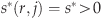
The aim of the whole collection process is to maximize the recovery rate—the amount collected as a fraction of the original debt. The definition of recovery rate can be extended to cover the recovery rate for each particular collections action as follows. Define  to be what is recovered by operating with action i for s periods as a fraction of the debt outstanding when action i was started. So
  . This is assuming that if action i is undertaken for s time periods, the amount recovered is a fixed percentage of the amount owed when the action started, and this percentage is independent of the type or duration of the previous actions applied to the debtor. So at the start of any action, the only part of the debtor's history that will affect future recoveries is the percentage of the debt already recovered. There is a collection cost for each period action i is undertaken and we define c
i
to be this cost expressed as a fraction of the original debt. We do not add this cost to the debt but we will subtract it from the total recovery rate to get the net recovery rate.
. This is assuming that if action i is undertaken for s time periods, the amount recovered is a fixed percentage of the amount owed when the action started, and this percentage is independent of the type or duration of the previous actions applied to the debtor. So at the start of any action, the only part of the debtor's history that will affect future recoveries is the percentage of the debt already recovered. There is a collection cost for each period action i is undertaken and we define c
i
to be this cost expressed as a fraction of the original debt. We do not add this cost to the debt but we will subtract it from the total recovery rate to get the net recovery rate.
The objective is to find the collections strategy that maximizes the net recovery rate from debtors, allowing for collections costs, where the cash recovered and the costs incurred are discounted by a factor β for each period into the future. We take the approach used by most reasonable lenders of freezing the amount of debt at default but recognizing that the subsequent cash flow of recoveries should be discounted to reflect the time value of money. Thus in almost all cases, the recovery rate will be <1. One can easily modify the model so that interest is charged on the unpaid debt, but the results obtained are very similar.
This problem can then be modeled as a dynamic programming problem. The decision epochs are the monthly reviews undertaken on each case to check what recoveries have occurred in the past month and what to do in the next period. We denote these review times as T={1, 2, …,}.  is the set of actions which the lender can use in seeking to recover a debt with the ordering described previously, so when using action i the lender cannot in future use actions j, j<i. These include contact by telephone or letter, agreement on repayment schedules using banking standing orders, and the threat and possibly the use of legal orders to recover property. We model the situation as an infinite time horizon problem rather than a finite horizon problem because the decision on when to cease collections and write off the debt will vary for different debtors. One way of dealing with this is to let the highest level action be to write off the debt, which has a cost of 0. The state space describes the situation at any time of an individual loan and consists of three components. These are the current action i being performed on that loan, the number of decision periods s for which that action has been undertaken so far, and r the recovery rate of the loan when this current action was started. With this definition, the transitions in the process are deterministic. If the lender keeps with the existing action, the expected increase in the recovery rate in the next period is
  and the process moves to state (r, i, s+1). If the lender decides to start another action immediately the process moves instantaneously to state (r+(1−r)F
i
(s), j, 0). Note that though we are modeling this problem deterministically and are interested in the optimal actions on the “average debtor” for resource purposes, the model gives a policy where the time in any action does depend on the recovery rate of that debtor when that action was started.
and the process moves to state (r, i, s+1). If the lender decides to start another action immediately the process moves instantaneously to state (r+(1−r)F
i
(s), j, 0). Note that though we are modeling this problem deterministically and are interested in the optimal actions on the “average debtor” for resource purposes, the model gives a policy where the time in any action does depend on the recovery rate of that debtor when that action was started.
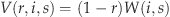
Define V(r, i, s) to be the future net discounted recovery rate given that currently action i has been performed for the last s periods and r is the percentage of the original debt that had been recovered when action i commenced. The net discounted recovery amount is the recovery amount less the costs of performing the actions, both costs and recoveries discounted by β for each period into the future. The net discounted recovery rate is the net discounted recovery amount divided by the amount of the original debt. The decision in state (r, i, s) is whether to continue with action i or to move to a more severe action. Hence  satisfies the following optimality equation of a dynamic programming model (Bertsekas 2007, Denardo 1982, Puterman 1994)
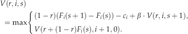
The first expression is the recovery rate if action i is continued for another period. The amount recovered in that period is  , because (1–r) is the fraction of the debt still to be recovered when action i starts. c
i
is the cost of action i and the recovery rate in subsequent periods is
, because (1–r) is the fraction of the debt still to be recovered when action i starts. c
i
is the cost of action i and the recovery rate in subsequent periods is  as the collection process starts the next period in state
  and the subsequent recoveries need to be discounted by one period. The second expression is what happens if it is decided to start action i+1 immediately. The recovery rate at the start of the action is
  , where the second term is what has been recovered from s periods of action i. Note that one does not need to consider more drastic actions than i+1 because in solving for the state (., i+1, 0) one will consider moving immediately to action i+2. Repeating this argument means one allows the possibility of moving immediately to all states (., j, 0), i.e., starting any action
  .
.
To find the optimal overall recovery rate and the optimal collections strategy, one must solve  , i.e., start with nothing recovered and having performed action 1 for 0 periods. Computationally this can be solved using value iteration, as outlined in the next section.
We have assumed a homogeneous population in the model but of course one could apply this at a subpopulation level and allow different types of subpopulations of debtors depending on their socio‐demographic characteristics, the type and amount of debt, and their previous credit history. The case study we discuss later has two such subpopulations.
3. Properties of the Optimal Collections Policy
There are some obvious properties one might expect of the relationship between the recovery rate and the duration of a specific collections action. Trivially one should expect
 is non‐decreasing in s.
A more debatable assumption is
 is concave in s (i.e.,
  is non‐increasing in s).
This is reasonable if i is a repetitive action like telephoning, where as time goes by the amount recovered from each telephone call gets less. It is the law of diminishing returns. The assumption may be less obvious for actions, which take some time to set up, like undertaking legal action for recovery of the debt. Once repayments have started though the condition would hold if the payments were constant each month but there was a positive chance each month of the debtor stopping paying and not restarting under that action.
The standard way of solving dynamic programming is to use value iteration where the iterates  are defined by
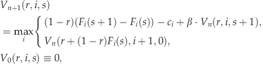
 converges to the solution of the optimality equation and this gives a way of solving numerically to find the optimal collections policy and the optimal recovery rate. To carry out this computation one discretizes the r values (we took 100 values, i.e., every 0.01 and used interpolation to obtain estimates of the values in between), while i and s are already discrete. Results in Puterman (1994) show that value iteration can solve problems with more than 1,000,000 states relatively easily, whereas our state space is in the low thousands. One can also use induction on the iterates of value iteration to prove results about the form of the value function and the optimal policy.
The first result explains how the optimal value function depends on the state descriptors  .
.
If A1 and A2 hold, then
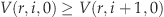
 is non‐increasing in r
 is non‐increasing in i
 is non‐increasing in s.
follows trivially because from (1)
Assume (i) holds for From A2, we have
 . The proofs of (i) and (iii) use induction on n the iterate of the value iteration procedure in Equation (2). Trivially all three conditions hold at n=0 because
  .
. then as r increases
 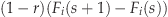 decreases and the induction assumption implies
  is non‐increasing. Summing these two gives that the first expression on the RHS of (2) is non‐increasing in r. As r increases
  increases and so
  is non‐increasing by the induction hypothesis. Hence,
  is non‐increasing in r and the induction holds.
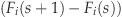 is non‐increasing in s.
  is non‐increasing in s because of the induction hypothesis. A1 implies
  is non‐decreasing in s and so (i) shows that
  is non‐increasing in s. Hence, all the terms on the RHS of (2) are non‐increasing in s and the induction hypothesis holds. □
These lemmas can be used to show that, under certain relationships between the costs and the recovery rates, the optimal collections policy has some obvious features. First note that the form of the optimality Equation (1) can be reinterpreted as follows. The optimal collections policy can be defined by a set of functions  , so that if the collection process starts action i, when the debtor's recovery rate was r, the action should be continued for
  periods, where
Note that if the current recovery rate is r, then there will be some actions j, with  which implies that action j will not be used. This is proved as follows.
If
 , then
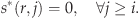
 , then as
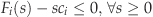
 in (1) and so
  . □
. □
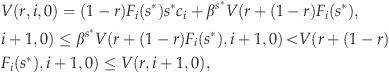
Note that if A2 holds and  , then condition (i) will also hold. Theorem 1 makes the point that the percentage already recovered r is sufficiently great, then one should not undertake a further action j if
  . This says the maximum recovery rate per period under action j does not exceed the cost of undertaking this action, but also means that for any action if the recovery rate so far is high enough it is not worth undertaking that action.
Finally, we prove the intuitive result that in the situation when  , one might as well run with each collection action for as long as possible before then moving on to the next hardest action, because there is no cost of operating any action and no penalty if the recovered amounts are very late in being paid.
 ,
,  .
.
 . Substituting this into Equation (1) yields an optimality equation for
  , namely
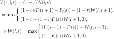
Note that 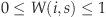 , as it is a recovery rate with no costs or discounts involved. To prove the theorem, it is enough to show that the first term in (3) is greater than the second term for all s. Now
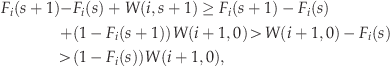
 . Thus one keeps on using action i all the time and so
  . □
. □
4. Case Study
The model developed in the previous sections was applied to collections data from a European Bank. The sample consisted of 3084 consumer loans that had defaulted over a 3‐year period. For each loan there were some details of the borrower, and loan details including when it was taken out, how much it was for, when the borrower defaulted, and how much was owed at default. There were also monthly details (covering 150,658 loan/months in total) of the collection process including which collection action was applied to the defaulter in the month and how much was recovered in that month.
There were five different collections actions recorded but in fact only three actions were ever considered for each debtor. This was because the collections process segmented the debtors into two groups depending on whether the defaulted amount was a low percentage of the original loan (which we will classify as G, the Goods) or a high percentage of the original loan (which we classify as B, the Bads). The policy was to allow actions 1G, 2G, and 3 to be applied to those in the Good group and actions 1B, 2B, and 3 were applied to those in the Bad group. Although not the same actions, 1G and 1B both concentrated on communicating with the defaulters and arranging repayment schedules. 2G and 2B are also different actions but both use legal procedures to recover the debt. The collection procedure has to begin with action 1G or 1B, because the regulations prevented collectors using legal procedures without first seeking to agree to a repayment schedule. As the collectors' objective is to maximize the recovery rate, allowing for collection process expenses they would want to move to stronger actions in due course. Action 3 is essentially passive in that the debt is kept on the books but no effort ( ) is made to recover the debt. The legal position in that country is that someone with an outstanding debt is not allowed to take out further credit and therefore many debtors do pay off their debt unsolicited (sometimes several years after the debt occurred) when they want to obtain further credit. Note that although action 3 is the weakest action, it still satisfies the modeling assumption that having moved to it, and written off the loan, the collector will not move subsequently to actions 1 or 2. We solve the problem separately for the two segments—Good and Bad.
The relationship between recovery rate and maturity was plotted for each action and from that it was felt that the exponential function 
 . It also had the advantage that the coefficients A
i
and B
i
are easy to understand, and so the collections managers were able to comment on whether they seemed appropriate in their experience. Coefficient A
i
is the recovery rate if the action was allowed to continue indefinitely while B
i
is related to the rate of recovery (
. It also had the advantage that the coefficients A
i
and B
i
are easy to understand, and so the collections managers were able to comment on whether they seemed appropriate in their experience. Coefficient A
i
is the recovery rate if the action was allowed to continue indefinitely while B
i
is related to the rate of recovery ( is the time until half the maximum possible recovery under this action will have occurred. The parameters A and B were estimated by estimating the average recovery rate during period s of action i for those debtors who were subject to action i for at least s periods. This gave an estimate of
 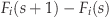 and by adding these estimates one could estimate
  . The parameters are then obtained by using non‐linear regression to fit the expression in (4) to these
  values.
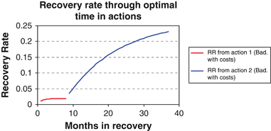
Figure 1 shows the form of the cumulative recovery rate function for 1G and 2G. Note that the estimate for 2G ignores how a debtor had performed on 1G. The estimated parameters for the Good segment were 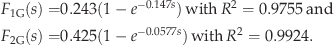
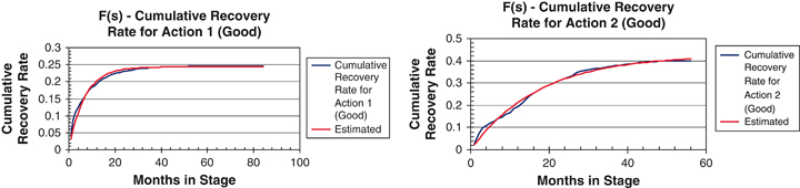
In the long run, action 2G collects more than 1G as it would eventually recover 42% of the debt outstanding while 1G would only recover 24%. However, 1G is quicker in recovering debt than 2G, recovering 14.2% of the debt outstanding in the first 6 months compared with 12.4% from 2G recovered in the first 6 months.
In the Bad segment, the cumulative recovery functions are similarly estimated. They are shown in Figure 2, where 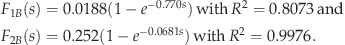
In this case, action 1B on average only recovers 1.8% of the debt outstanding when one starts applying that action even if it was used forever, whereas action 2B could recover 25% of what is owed if it was operated forever. So really action 1B is extremely unsuccessful and 2B is far less successful than 2G, though this has more to do with the difference between the debtor types rather than any difference in the actions.
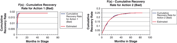
Action 3, which involved no proactive collection procedures, was the only action where plotting the data did not give a good fit to the exponential function. Investigation also suggested only minute differences between the results for the two groups, Good and Bad, and so it is considered that the same action (or perhaps non‐action is a better description) is applied to both groups. As there are no costs in this action and no “harsher” action can be undertaken once a debt reaches this state, there is no point in ever stopping doing this action. Figure 3 shows the debtors' repayment behavior under action 3. We sought to fit it using a combination of linear functions and the exponential function which fitted the other actions so well. The result was a curve of the form 
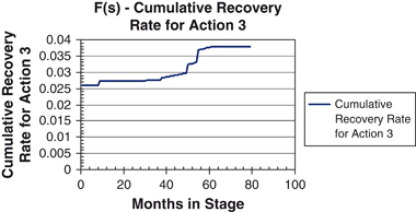
Note that the recovery rate for this action is extremely low—just 3% recovered in the long term—which is not surprising because there is really no interaction with the debtor.
In calculating the cost c
i
of operating the various actions, one has to use expert judgment. The monthly cost of each operation was determined having examined the whole collections budget and after discussions with the collections managers. c
i
though is this cost expressed as a fraction of the debt outstanding on default, and to do this we took the average balance at default of those who were in the Good group (for  ) and in the Bad group (for
  ). This resulted in estimates of the costs of
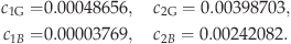
There were data for up to 80 months in the collection process with up to 60 months available on individual actions. It was clear that almost all collection actions achieved no further recoveries after 48 months (some of them such as 1B stopped well before). So it was decided to let each action take place for a maximum period of 48 months, i.e., 4 years.
Looking at the case where the costs are given by Equation (5), but the discount factor is chosen to be β=1, we obtain the results in Table 1 for the Bad segment of debtors and the results in Table 2 for the Good segment.
Of course for resource allocation purposes, we are only interested in the case when the recovery rate before the first action is 0, in which case the second action starts after 8 months with an expected recovery rate of 0.0188 from the first action. We have added the results for how long the collectors should undertake the second action 2B if the recovery rate in the first action is not this average value for sensitivity analysis purposes. The column “Recovery rate after 1B applied” shows reference values of recovery before the start of action 2B, and the rest of the row described how long 2B should be undertaken and the effect it has on the net recovery rate. Table 2 describes the same results for the Good segment of debtors. The total recovery rate in the penultimate column is the total percentage of the debt recovered while the optimal net recovery rate in the final column includes the cost of the recovery process. The results are that for the Bad segment one can expect an optimal net recovery rate of 18.3% (including costs) by applying action 1B for 8 months followed by action 2B for 29 months before moving the debt into action 3 (the passive action) where it can stay indefinitely. Twenty‐two percent of the debt should be expected to be recovered by action 2B though. Figure 4 shows this optimal recovery rate as a function of the months into the collections process for the Bad type of customers. It highlights how much of the recovery comes from action 2B compared with action 1B.
The results in the Good segment are quite different as Table 2 shows. One would expect to recover 51% of the debt eventually and the optimal policy is to operate with action 1G for 29 months followed by action 2G for another 27 months before moving the debt to the passive state. In this case almost equal amounts of debt are recovered by the two types of actions.
This policy could be compared with another policy, such as using action 1G for 1 year, followed by action 2G for another year and action 3 indefinitely. This policy would collect 39.0% of the debt instead of the 51.0% recovered using the optimal policy. The net recovery rate would be 33.6% using this policy and 38.8% using the optimal policy. Note that the optimal policy can recover 12% more of the debt than this other policy but half of the “extra” amount recovered is used up by the extra collection effort so the net improvement is just over 5% of the outstanding debt. Figure 5 shows the optimal recovery rate as a function of the months in the collection process for the Good segment. In this case the amount collected in the first 29 months using action 1G is almost as much as is collected by using 2G in the remaining 27 months.
Note that in both Tables 1 and 2, as the recovery rate from action 1 increases the time in action 2 drops. This is because there is less debt still to recover and so the operating costs are a larger proportion of the possible amount to recover. Of course the total net recovery rate increases as the amount recovered in action 1 increases but the amount of this that comes from the second collection action decreases. If a sufficient amount has been recovered from the first action, it may not be worthwhile undertaking the second collection actions at all. This is the case for action 2B in the Bad segment if at least 90% of the debt has been collected by action 1B. Similarly for the Good segment, one would not use 2G if 84% of the debt had been recovered before its operation.
If we introduce discounting with the monthly discount factor set at β=0.99746 (corresponding to an annual inflation rate of 3.2%—the European average for the last 5 years), the results are very similar as Tables 3 and 4 show. The main difference is that the optimal recovery rates are slightly lower because of the time before one starts to recover some of the amounts. Also the durations of the first action drop a little because, especially in the Bad segment, one wants to move more quickly to action 2B which is where the main recovery occurs so that the recoveries are not too heavily discounted.
Optimal Policy for Good Segment with Costs and Discounting
5. Conclusions
It is surprising that so little research has been undertaken into the operations management of the collections process in consumer credit. This may well be psychological in that banks want to “bury their mistakes” but it is also partly the accounting conventions in that when a bank has written off all or part of a loan, senior managers are only concerned that the write‐off covers the loss and are less concerned with minimizing the loss by optimizing the subsequent collections process. Also the collections process is sometimes contracted out or sold on to other debt recovery organizations and so the data on collections are not available. Even when collections is kept “in house,” collections departments tended to register only the most basic information on the process.
The model introduced here is essentially a homogeneous one in that difference between debtors is only allowed for by segmentation and within a segment, the population is assumed to be homogeneous. This model is useful as a way of identifying what the cash flow from recoveries would be under the optimal collections process. Such information together with estimates of numbers of new debtors moving into collections each month is what is required for provisioning. The model is also useful in determining the allocation of resources within the collections department to obtain this optimal average recovery rate under the different actions.
One could expand the problem by seeking to tailor the collections process to the individual debtor, but one would then need to connect the cumulative recovery rate function for each action to the characteristics of the debtor. This will require experimentation by collections departments to acquire this data, but will be worthwhile doing once such data becomes available. One might also want to expand the model by including the information on the recoveries to date from an individual debtor from the current action being applied in deciding whether to continue that action or not. For example, if someone is keeping to the agreed restructured repayment pattern, one would not want to change this; if someone has been repaying more than the average so far under a particular action one would want to keep with that action even if for the average debtor it is time to change to another approach. There are parallels with the way one adjusts the credit limits for borrowers who are repaying satisfactorily in the light of movements in their behavioral score. As it has taken many years for such operating decisions to be based on behavioral scores, it should not be expected to happen overnight with the collections equivalent problem. The need is to acquire collections data in this level of detail.
Another extension will be to move from the way of modeling recoveries repayment to modeling it as a stochastic process. Part of this would mean checking what impact the previous recovery actions have on the efficacy of the current action. Our model assumes that they have none but that one can never return to a previous action. Checking whether the recovery process is really “memoryless” in this sense and that returning to previous actions is pointless would be part of developing such stochastic models.
Data are the key. Without it no useful model of the collections process can be built. Some collectors are investigating the use of text mining to identify the key phrases in the recorded conversations between debtor and collector, which will categorize those who will subsequently repay the debt and those who will not. Most collections departments though are nowhere near this level of sophistication and a useful first step would be to collect and keep the data which were needed in this case study—the records of what collections actions were performed on the debtor that month and how much of the debt the debtor repaid in that month. With that, collections departments would be in a position to improve the operations of their processes by models akin to that developed here.
Footnotes
Acknowledgments
This work was partially supported by CAPES (Coordenação de Aperfeiçoamento de Pessoal de Nível Superior, a Brazilian Research Agency under the Ministry of Education of Brazil).
We would like to thank the referees for their valuable contributions.