Threshold Incentives and Sales Variance

Abstract

In this paper, we analyze the impact of two forms of commonly used threshold‐based incentive schemes on the observed sales variability. The first form of the incentive comprises an additional marginal payment on crossing a specified sales threshold and the second form of the incentive scheme comprises a lumpsum bonus payment on crossing the predetermined sales threshold. We model the effect of such incentives under two specific scenarios: an exclusive dealership selling a single product and a non‐exclusive dealer selling two competing products. For an exclusive dealer, we show that a bonus contract not only increases the expected sales, but, more importantly, decreases the sales (order) variance. Consequently, the bonus‐based scheme allows the manufacturer to regulate sales variance better. With a non‐exclusive dealer, the sales variance increases substantially with an additional marginal payment contract. However, our analysis suggests that the bonus contract continues to perform better in this case, too, if the threshold level is set appropriately using the underlying demand distribution.

Keywords

threshold incentives service and supply chain operations sales variance

1. Introduction

Quota‐based compensation plans are widely used in practice to motivate the sales‐force to increase sales. One example of a threshold‐based¹ sales‐force incentive mechanism is the so‐called stair‐step incentive offered by auto manufacturer Chrysler to its dealers (Post‐Distpatch 2001). Under this incentive plan,² Chrysler gave dealers cash based on a percent of the monthly vehicle sales target met. It is commonly believed that such threshold‐based incentives are effective in increasing a manufacturer's expected sales and profit while motivating the dealer to exert effort appropriately. But it has also been observed that poorly designed incentives can increase the sales variance causing the manufacturer substantial difficulty in production planning, inventory management, and distribution costs. This may potentially increase a manufacturer's operational cost. As is well known in the operations management literature, higher variability in the demand process affects over‐stocking and under‐stocking costs. In this paper, we take the position that manufacturing and distribution costs increase with sales variability. Thus, it is in the manufacturer's interest to regulate the observed sales variability.

The desire of this work is to study the impact of threshold‐based contracts on the sales variance observed by the manufacturer. To this end, we have not explored the issue of the optimal contract to maximize the total profit (considering the effect of sales variance) of the manufacturer. Rather, we draw insights about the impact of these contracts on the variance of the observed sales (demand) that hold regardless of the production and distribution costs at the manufacturer. To do so, we consider two types of such sales‐force compensation plans: (1) when the dealer (salesperson) is paid an additional amount per unit when sales exceed a threshold value, and (2) when, instead of an additional per unit (marginal) payment, a fixed bonus is offered if the total sales exceeds the threshold. We refer to the first form of the threshold contract as a marginal payment contract and to the second form as the lumpsum bonus contract. These two forms are commonly observed in several industries. Sinha and Zoltners (2001) provide evidence of marginal payment sales‐force compensation schemes widely used in industries such as pharmaceutical, media, and telecommunications. The bonus‐based incentive plan is quite popular in industries such as electronics and retail (Joseph and Kalwani 1998). Bonus payments have helped firms direct sales‐force effort toward specific organizational goals and increase productivity. The Chrysler plan described earlier is a combination of the marginal payment and bonus plan.³ It is also interesting to note that quantity discount schemes, which are widely used in practice, are similar to threshold‐based contracts. Typically, in such settings the retail price of the product is fixed and the manufacturer (or the supplier) specifies a quantity discount if the dealer (retailer) procures more than a predetermined threshold value. This translates to a setting where the profit margin that the dealer (retailer) obtains by selling a marginal product depends on whether he is above the threshold or not—a setting similar to the marginal payment threshold‐based incentive. Some additional examples can be found in Xiao (2007). For example, to promote sales of storage switches Cisco returns 5% of the wholesale price back to its resellers if the sales in a quarter are higher than 20% of the previous quarter. Similarly, Xerox, under its Xtra partner program, provides a 4% rebate for every unit of sales if the sales exceed US$1 million.

In this paper, we show that threshold‐based contracts lead to uneven sales effort by characterizing the dealer's optimal response (effort levels) when the underlying demand is uncertain. To analyze the issue of sales variance, we consider two supply chain settings. First, we consider a setting when the dealer sells a single product exclusively for a single manufacturer, i.e., the dealer does not sell competing products. In this case we show that the manufacturer benefits by offering a lump sum bonus contract if she chooses to regulate the sales (order) variance. On the contrary, the additional marginal payment contract is unable to lower the sales variance. Moreover, as the demand variability increases, the gap between the sales variance and the underlying demand variance also increases. This has a few implications for the incentive provider. For example, it may be beneficial to invest some effort to control the underlying demand variance. Second, we study the case when the dealer is non‐exclusive, i.e., the dealer (salesperson) sells perfectly substitutable products (possibly from competing manufacturers). For example, auto manufacturers are increasingly dealing with non‐exclusive dealerships in the United States. In this case, we show that a threshold contract with an additional marginal payment is once again unable to lower the sales variance. However, it is possible to regulate the sales variance with a bonus contract. Through numerical experiments we demonstrate that the observed sales (order) variability for a particular product can be regulated better with a properly designed lump sum bonus contract.

Overall our analysis highlights the following observations about threshold‐based incentives. The increase in the sales variance with a marginal payment contract is primarily due to the sales threshold specified in the contract. These results supplement some of the findings in Sinha and Zoltners (2001) and Zoltners et al. (2006) where the authors provide a detailed discussion on why setting incorrect sales goals can be very costly for a firm. In such a case, using a different form of the contract, such as a fixed‐margin contract without a sales threshold, may be beneficial for the manufacturer if she is concerned about sales (order) variance. In the case of a lump sum bonus contract our results suggest that, by appropriately choosing the sales threshold level based on the underlying demand distribution, the manufacturer is able to regulate sales variance better. However, it is noteworthy that, if the incentive threshold is not linked to the market demand, the resulting variance of sales can be higher with a bonus contract, too.

The rest of the paper is organized as follows. In section 2 we provide a literature review. We discuss the model and its assumptions in section 3. We analyze the case of the exclusive dealer in section 4. We then analyze the case of a non‐exclusive dealer in section 5. For brevity of exposition we only include the key results regarding the optimal effort regions and sales variance. A detailed analysis is provided in the supporting information appendix (see Appendices S1 and S2). Finally, we conclude the paper with a short discussion of our results in section 6. Proofs of all the propositions and lemmas are provided in the Appendix.

2. Literature Review

The theoretical literature, in economics and marketing, provides evidence that threshold‐based incentives are effective (and optimal in some cases) in increasing a manufacturer's expected sales while motivating the dealer to exert effort appropriately (Basu et al. 1985, Kim 1997, Oyer 2000, Sappington 1983). However, many of these single time period models ignore the impact on operational sales variance. In the model discussed in this paper, we focus on the issue of observed sales variance and compare which form of the threshold‐based contract performs better on this dimension.

Basu et al. (1985) study the sales‐force compensation plan for a single period and show that the optimal compensation plan is an increasing non‐linear function of the sales (BLSS plan). Basu et al. (1985) also suggest that, for ease of implementation, a piecewise linear approximation scheme could be used in practice. Such a scheme closely resembles the threshold‐based incentive studied in this paper. The analytical approach in Basu et al. (1985) follows the moral hazard and agency theoretic framework adopted in Harris and Raviv (1979) and Holmström (1979). Raju and Srinivasan (1996) compare the BLSS plan to a simple quota‐based plan (fixed pay plus a commission rate) and show, through numerical experiments, that their simple approximation results in minimal loss of optimality. The significant advantage, as argued earlier, is the simplicity of implementation in practice. Lal and Srinivasan (1993) find that a linear compensation scheme may be optimal; however, such a scheme seems impractical because most sales‐force incentive schemes in practice are non‐linear. In a related paper Oyer (2000) shows that a quota‐based plan with a bonus payment is optimal when the sales distribution function is assumed to have an increasing hazard rate. Through field experiments, Joseph and Kalwani (1998) demonstrate the growing importance of bonus payments in aligning sales incentives and increasing productivity in a wide variety of firms. In this paper, we assume a model similar to the model described in Oyer (2000). In our case, though, the dealer chooses his optimal effort level after observing his private demand. Detailed reviews on the sales‐force management literature can be found in Coughlan and Subrata (1989) and Coughlan (1993).

More recently, the literature in operations management has focused on the operational impact of such quota‐based contracts (Chen 2000, Lee and Tang 1996, 1998) and suggested strategies to smoothen the demand process. Chen (2000) discusses the impact of sales‐force incentives, over multiple time periods, on a manufacturing firm's production and inventory decisions and proposes a moving‐window plan to induce salespeople to exert selling effort to smoothen the demand process. In their paper the sales surge observed is because the dealer does not experience any additional cost of postponing the effort decision and hence exerts all the effort in the last period. In this case, the dealer waits for the exogenous stochasticity in the demand to resolve itself before making any effort. This results in the sales spike that is observed only in the last period whereas all the earlier‐period sales are unaffected. In a following paper Chen (2005) relates sales‐force compensation to the manufacturing firm's production and inventory costs and compares Gonik's scheme with a menu of linear contracts. Gonik (1978) proposed a scheme to extract maximum effort from the sales‐force and induce them to truthfully reveal the underlying demand by forecasting accurately. In contrast, as described earlier, we focus on comparing the two forms of threshold‐based contracts and study which form controls sales variance better.

In other related work Xiao (2007) studies all‐unit target rebates (similar to the Chrysler example discussed in section 1) and incremental‐unit target rebates (similar to our additional marginal payment) in a single period setting where the manufacturer is a Stackelberg leader specifying the terms of the incentives. In their stylized setting, similar to the model setting in this paper, the retailer makes his effort decision after the market condition is realized. Xiao (2007) finds that, from the manufacturer's perspective, the expected profit from an all‐unit rebate contract is dominated by a wholesale price contract, which in turn is dominated by an incremental‐unit target rebate. Xiao (2007) does not specifically incorporate the issue of sales variance. As mentioned earlier, our focus is on the additional sales variance induced because of such contracts. There is substantial operations management literature available on the role of information sharing in supply chains and how it helps to smoothen the observed ordering pattern and benefit the incentive provider. For example, Lee et al. (1997) quantify the benefits of information sharing through inventory reduction and cost control. They show that information sharing allows controlling the variance of the orders. We take a similar position in this paper that if the manufacturer is able to control the demand variance then she is better off.

3. Model

The exclusive dealer setting is similar to the case where a dealer sells a single product for a manufacturer. In this section, we begin by describing the exclusive dealer setting first and then describe the non‐exclusive dealer setting. For simplicity we consider the selling price of the product to be fixed and exogenous. Thus, the only way for the dealer to grow sales is to exert effort. For example, the dealer could expend selling effort through advertising. As the retail price is held fixed, the dealer makes a standard margin (excluding cost of effort) p for every unit sold. However, to a limited extent, the dealer's ability to increase sales by lowering the retail price (and decreasing his standard margin) is approximated by the additional cost of exerting sales effort to increase sales.

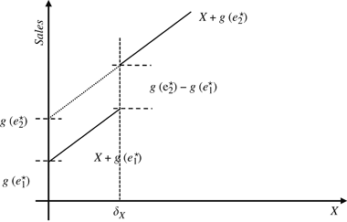
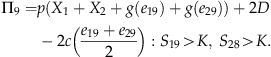
The dealer chooses a selling effort e resulting in a sales growth of g(e), where the impact‐of‐effort function, g(·) is positive, differentiable, increasing, and strictly concave. Therefore, the marginal impact of sales effort is diminishing. The sales, S, is assumed to be 1 where X is the random demand (shock) observed by the dealer. We assume that the market demand signal, X, follows a continuous, and twice differentiable, cumulative distribution function, F, with a probability density function f such that f(X)=0 for all X<0. The distribution of the market demand signal is common knowledge (publicly known). Such a sales response function, as shown in (1), has also been used by Lal and Staelin (1986), Oyer (2000), and Lal and Srinivasan (1993). The dealer's cost of exerting effort, c(e), is assumed to be strictly positive, increasing, and convex in his effort. We also assume that c′(0)<g′(0) and that the set {e: pg(e)−c(e)≥0 and e≥0} is non‐empty and convex.

The threshold incentive is organized as follows: For every additional unit sold above the threshold, K, the manufacturer pays the dealer an amount Δ in addition to his standard margin p. Thus, the dealer's margin (excluding the cost of effort) increases to p+Δ for every unit sold above the threshold K. We refer to this contract as the “Δ‐contract.” In case of a bonus contract, instead of the additional marginal payment, Δ, the manufacturer offers a fixed bonus, D>0, if the total sales, S, reaches, or exceeds, the threshold K. We refer to the bonus contract as the “D‐contract” and consider it separately. The incentives offered are represented by their defining parameters, i.e., (p, Δ, K) represents the Δ‐contract and (p, D, K) represents the D‐contract.

The dealer's objective is to maximize his expected profit, which is a function of the effort exerted, the incentive parameters, and the profit margin. The sequence of events unfolds as follows. The manufacturer offers the dealer the contract. The dealer observes his market demand signal and chooses his optimal effort level. The manufacturer then observes the total sales and payoffs are made based on sales. We assume that the manufacturer keeps finished‐goods inventory and is responsible for replenishing the dealer's inventory.

The non‐exclusive dealer setting is similar to the situation when the dealer sells two perfectly substitutable and competing products. This situation can be viewed as products from two competing manufacturers or two competing products from the same manufacturer. We use the former context throughout our discussion. Consequently, we use the term product and manufacturer synonymously to identify how the non‐exclusive dealer splits his effort. To keep our analysis focused, we assume that the efforts exerted across the products are perfectly substitutable and also assume that each manufacturer offers a similar threshold‐based incentive to the dealer, i.e., each product is associated with threshold‐based incentive schemes with identical parameters. The non‐exclusive dealer observes two market signals X _i, i=1, 2 (one for each product i), and then decides on the effort levels e _i, i=1, 2, across the two products. Our analysis assumes that the market signals across the two products are independent. The sales for each product, i=1, 2, are S _i=X _i+g(e _i). The dealer's cost of the effort is based on the total effort across the two products and is assumed to be where c(·) is a strictly increasing, positive valued, convex function in its argument. It is reasonable to assume that the dealer's cost is a function of the total effort (average) because common resources are used by the dealer to spur sales across all the products sold. If the optimal efforts exerted are completely symmetric, then the cost function allows us to model the fact that the non‐exclusive dealer faces similar costs as two independent exclusive dealers. For all other cases, the function models the fact that the overall cost is slightly lower due to economies of scale.

Finally, we would like to comment about the sales response function (1). We assume an additive model where the period sales is the sum of a random demand and an increasing function of the effort deployed by the dealer. In reality, it is plausible that the impact of the effort is more complex (such as a combination of an additive and a multiplicative form), but as we mention earlier the additive response model has been commonly used in the previous literature to capture sales growth and also to have analytical tractability. With an additive sales response function, it is possible to separate the dealer's optimal effort levels from the underlying demand signal. Further, one can envision a more generalized model where the dealer effort results in a random increase in sales. However, if this increase is additive, then this general model can be reduced to the model described above.

During our analysis we do not explicitly model the manufacturer's objective function. As mentioned earlier, we draw insights about the impact of such threshold‐based contracts on mean and variance of the observed sales that hold regardless of the production, inventory, and distribution costs at the manufacturer.

4. The Exclusive Dealer

In this section we consider the case when a dealer sells only a single product (i.e., from a single manufacturer). Our goal is to characterize the impact of the threshold‐based incentives on the sales. We begin by first characterizing the exclusive dealer's optimal sales effort.

4.1. The Exclusive Dealer's Optimal Response

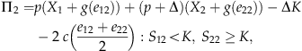
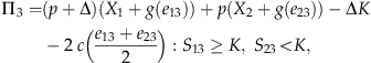
Recall that the dealer makes the decision on the effort, e, after observing the market signal X. Thus, the dealer's choice of effort leads to one of the two possible outcomes in terms of sales: S<K or S≥K. Let us first consider the Δ‐contract.

4.1.1. The Δ‐Contract. With a Δ‐contract the dealer's profit, depending on the sales outcome, can be characterized as follows: 2 3

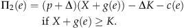
Observe that Π₁(e) and Π₂(e) are concave in the effort e. Using this fact we derive the dealer's optimal efforts in Lemma 1. The derivation relies on the first‐order optimality conditions and we do not formally state the proof. Lemma 1 also characterizes the demand signal level (cutoff on X), δ _X, above which the dealer switches to the higher effort level .

Lemma 1. With a Δ‐contract the dealer's optimal effort is characterized as follows: 4 where and the demand signal δ _X beyond which the dealer switches his effort from to is given by 5 where 6

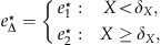
It is noteworthy that due to an additive sales response function the dealer's optimal efforts are independent of the underlying random demand signal. Note that Lemma 1 implicitly states that the dealer will always exert an effort such that the marginal benefit of exerting such effort equals the marginal cost of effort in this range of demand signals. However, for higher values of the demand signal (when it is optimal to exert effort such that sales exceed the threshold K), the dealer exerts a higher effort such that the marginal cost of effort, , equals (p+Δ) . 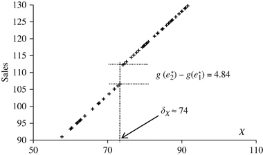Consequently, for a Δ‐contract, the dealer chooses between the two optimal effort levels, and , depending on the demand signal level. Figure 1 shows a schematic representation of sales as a function of the demand signal X. The sales are higher when X≥δ _X. We demonstrate this sales pattern using numerical experiments later. Next, we consider the D‐contract.

Figure 1

The Optimal Effort Levels and Sales for a Δ‐Contract

4.1.2. The D‐Contract. With a D‐contract the dealer's profit functions are as follows: 7 8

Consequently, the choice of the optimal effort is slightly different. As argued earlier, the dealer at least exerts the lower effort level for all market signal levels. However, there is a range of intermediate market signals when it is optimal to just reach the threshold K to capture the fixed bonus payment D. In this range the dealer exerts effort e _X ^K such that X+g(e _X ^K)=K. It is worth noting that in this range the sales level is constant as the dealer continuously varies his effort level to just reach the threshold K. Thus, with a D‐contract, there are two cutoff levels, δ _X1 and δ _X2, such that the dealer exerts the lower effort for all market signals in the ranges X≤δ _X1 and X≥δ _X2. However, he continuously varies his effort for intermediate signals δ _X1<X≤δ _X2 to raise the sales up to K. Of course, when X≥δ _X2 the dealer switches back to the lower effort e ₁ ^r because the demand signal is high enough to capture the bonus payment and there is no need to exert additional effort. In Lemma 2, we characterize the dealer's optimal effort levels under a D‐contract and also derive the demand signal cutoff values where the shift in effort levels takes place.

L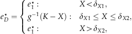emma 2. With a D‐contract the dealer exerts his optimal effort as follows: 9 where 10 11 and γ _X is the unique solution to 12 such that .

Note that, in Lemma 2, the dealer's optimal effort is higher than in the range δ _X1<X≤δ _X2 and depends on the magnitude of the bonus payout D. Moreover, the dealer's effort is continuously varying in this range but the resultant sales are held constant at K. We illustrate the optimal effort and sales pattern through numerical experiments later. Using the optimal effort levels derived in Lemmas 1 and 2 we analyze the variance of sales next.

4.2. Observed Sales Variance

Given the dealer's choice of optimal effort levels discussed in section 4.1, our goal in this section is to study the variance of sales for different forms of the incentive offered by the manufacturer. Let and denote the mean and variance of the underlying demand signal, respectively. Furthermore, let and denote the expected sales and variance of sales under a Δ‐contract and let and denote the mean and variance of sales under the D‐contract, respectively. We assume that the manufacturer chooses a threshold because, if this is not the case, the dealer always exceeds the threshold K and gains.

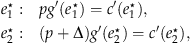
We first consider the sales variance with a Δ‐contract in Lemma 3. Recollect the definition of ɛ _X in (6).

Lemma 3. For anyΔ‐contract

(i)

, and

(ii)

Lemma 3 demonstrates that the manufacturer is unable to regulate the sales variance with a Δ‐contract. The sales variance is primarily higher due to the sales threshold. Consequently, the benefits of higher expected sales are offset by the resulting higher operational sales variance.

Next, in Lemma 4 we show that for a reasonably large range of the threshold K, the variance of sales with a D‐contract is strictly lower than the underlying demand variance.

Lemma 4. For any D‐contract .

Lemma 4 highlights the fact that by properly choosing the parameters of the D‐contract the manufacturer is able to reduce the sales variance below that of the underlying demand signal. Essentially, by using a D‐contract, the manufacturer can induce the dealer to exert effort in a way that smoothes her sales (order) pattern.

4.2.1. Numerical Experiments. In this section we demonstrate our sales variance results, using numerical experiments, for the Δ‐contract and D‐contract. For these experiments p=150, g(e)=e ^0.5, c(e)=0.001e ². With the Δ‐contract we fix Δ=75. Consequently , , and ɛ _X=2.313. Recollect that the cutoff 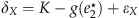. Figure 2 illustrates the sales pattern. Observe that the pattern is similar to that described in Figure 1 earlier. The dealer switches to the higher effort level when X>δ _X. Figure 3 shows the variance of sales for different demand signal distributions. The demand is assumed to be normally distributed with (we only change the mean). To highlight the gap between the variance of sales and the variance of demand, is shown by the dashed line at the bottom in the figure. Observe that when K is small compared with (plot with ) the sales variance is closer to . In this case it is not profitable for the dealer to vary his effort to reach K. As the coefficient of variance of X increases the gap between and also increases, i.e., the resulting sales variance is higher. The results of these numerical experiments have important implications for the manufacturer. If the demand variability is reduced, the variability of observed sales can be regulated. Thus, the manufacturer should consider investing in instruments that help in controlling the underlying demand variability. The idea is similar to examples in the operations management literature that describe benefits of the reduction in demand variability by modifying process or product attributes (Lee and Tang, 1996, 1998) or by information sharing (Lee et al. 1997).

Figure 2

The Sales Pattern for a Δ‐Contract (p=150, g(e)=e ^0.5, c(e)=0.001e ², and Δ=75)

Figure 3

The Observed Sales Variance for a Δ‐Contract at Different Levels of K and (p=150, g(e)=e ^0.5, c(e)=0.001e ², and Δ=75)

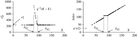
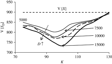
Next, we consider the D‐contract. The plot to the left in Figure 4 illustrates how the effort varies as demand signal X varies. For these experiments we keep the distribution of X fixed, i.e., normal with a mean of 100 and standard deviation of 30. However, we vary D and K. While all other parameters are as before, we only change c(e)=0.01e ². Consequently changes to 241.37 and . Observe that between δ _X1 and δ _X2 the effort level continuously decreases from g ⁻¹(γ _X) to . The plot to the right shows the sales as a function of the demand signal X. The total sale is constant at K when δ _X1≤X≤δ _X2.

Figure 4

The Optimal Effort and Sales for a D‐Contract (p=150, g(e)=e ^0.5, c(e)=0.001e ², and D=5000)

The plots in Figure 5 show variance of sales for different levels of D=5000, 7500, 10,000, 15,000. As can be observed, the variance of sales is lower than for all values of 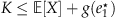and the gap between the two increases and D increases.

Figure 5

The Observed Sales Variance for a D‐Contract at Different Levels of K and D (p=150, g(e)=e ^0.5, c(e)=0.001e ²)

Having established that a D‐contract performs better than a Δ‐contract in regulating the sales variance with an exclusive dealer, we now focus our attention to when the dealer sells products from competing manufacturers and can shift his effort.

5. The Non‐Exclusive Dealer

Our goal is to understand how the loss of exclusivity affects sales variance for manufacturers offering threshold‐based incentives. Earlier in section 4 we proved that with an exclusive dealer the manufacturer is able to regulate sales variance better with a D‐contract. However, there are several instances in practice when the dealer may not be exclusively selling a single manufacturer's product. In such a non‐exclusive setting we assume that the effort exerted by the dealer is perfectly substitutable across the competing products. From the non‐exclusive dealer's perspective the ability to adjust sales effort is more profitable because the dealer can now allocate more effort to selling the product whose demand is higher. However, an important question for the manufacturer is whether she faces higher sales variance due to shifting dealer effort. Essentially, do the threshold‐based incentive schemes hurt or help in controlling the resulting sales variance?

To keep our analysis simple we also assume that the product demands are independent and identically distributed. In our model dealers that sell products for different manufacturers from different physical inventory lots are also non‐exclusive as long as they can shift sales effort across the manufacturers. This often occurs in practice because a dealer selling for two manufacturers is likely to shift incentives and advertising effort cost across the manufacturers depending upon market conditions. To this end, consider two manufacturers (1 and 2) selling their products (also denoted by 1 and 2) through a single non‐exclusive dealer. For expositional convenience we assume that both manufacturers offer similar threshold‐based incentives.

5.1. Observed Sales Variance

Similar to the exclusive dealer case, the non‐exclusive dealer observes the demand signal for both the products he is selling and then chooses his effort appropriately. Let X ₁ and X ₂ denote the demand signals observed for products 1 and 2, respectively. First we analyze the case when both the manufacturers offer a Δ‐contract.

5.1.1. The Δ‐Contract. We begin by enumerating the possible sales outcomes and the resulting dealer profit functions. Let the index i=1, 2 represent the products (manufacturers) and j represent the possible profit outcome for the dealer. Let S _ij=X _i+g(e _ij) represent the observed sales for product i corresponding to profit Π_j. The four possible outcomes correspond to the regions of demand signals X ₁ and X ₂ such that (1) S ₁₁<K and S ₂₁<K, (2) S ₁₂<K and S ₂₂≥K, (3) S ₁₃≥K and S ₂₃<K, and (4) S ₁₄≥K and S ₂₄≥K. 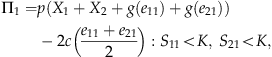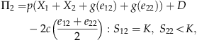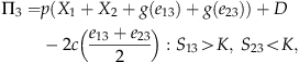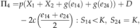Thus, with a Δ‐contract, there are four possible profit outcomes for the dealer, Π_j (j=1, …, 4), with four distinct optimal effort levels (j=1, …, 4) for each product i=1, 2. 13 14 15 16

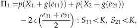
It is verifiable that each profit function Π_j is concave in the effort levels e _1j and e _2j, respectively. We include the complete technical analysis in the accompanying supporting information appendix (see Appendix S1). In this section, however, we simply summarize our analysis in Lemma 5. Recollect the definitions of the optimal efforts and in (4) for the exclusive dealer case.

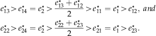
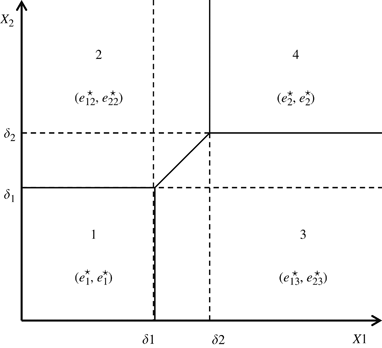
Lemma 5. With any given Δ‐contract the non‐exclusive dealer's optimal efforts are nested as follows:

It is noteworthy that, due to an additive sales response function, the dealer's optimal efforts are independent of the underlying random demand signal. Figure 6 illustrates the four profit regions (j=1, …, 4) and shows the optimal effort levels described in Lemma 5. Recollect the definition of the cutoff δ _X in (5) for the exclusive dealer case. δ ₁ and δ ₂ are similar cutoff values on the market demand signals X ₁ and X ₂ that determine the regions 1, 2, 3, and 4 as shown in the figure. Moreover, δ ₁<δ _X<δ ₂. We fully characterize these cutoff values in the supporting information appendix (see Appendix S1). In regions 1 and 4, the dealer exerts the lower effort, , and higher effort, , respectively. But, for an intermediate band (region between the cutoffs δ ₁ and δ ₂), when the demand signal for product 2 is higher than that for product 1, the dealer stretches to increase the sales for product 2 by shifting effort from product 1. Essentially, the dealer exerts a higher effort for the product with a higher market signal because he has an additional incentive to capture the higher marginal profit on reaching the threshold. Thus, as we show in the supporting information appendix (see Appendix S1), the non‐exclusive dealer's expected profit is higher than the case with two exclusive dealers selling these products independently. However, as the non‐exclusive dealer adjusts his effort across the products, the manufacturers observe higher sales fluctuations.

Figure 6

The Optimal Effort Levels for a Δ‐Contract

We now focus on the sales variance observed by the manufacturer for product 1. Similar to the exclusive dealer's case let represent the variance of the demand signal for product 1 and represent the observed sales variance for product 1. Next, in Lemma 6, we analytically establish that in general for any distribution.

Lemma 6. With a Δ‐contract, in the case of a non‐exclusive dealer, .

As Lemma 6 demonstrates, even with a non‐exclusive dealer, the manufacturer is unable to regulate sales variance using a Δ‐contract. As with the exclusive dealer case, the increase is primarily due to the fluctuating sales effort to reach the sales threshold. An important issue is to understand the magnitude of the increase in the sales variance. To this end, we conduct numerical experiments using normal and uniform distributions for the underlying demand. In the plots in Figure 7 we show how varies when X ₁ and X ₂ are uniformly distributed. We consider three cases where takes the values 75, 100, and 150, respectively. In all these experiments . The parameters of the experiments are as follows: p=150, g(e)=e ^0.5, Δ=75, and c(e)=0.001e ². Using these parameters the optimal efforts are , , 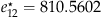, and . The profit regions depend on the value of threshold K that is varied from 100 to 160 in these experiments. As is readily observable from Figure 7, is strictly positive and increases with K initially. However, as K increases beyond a point the dealer does not find it profitable to switch effort and consequently only exerts . As a result, the sales variance starts decreasing. It is noteworthy that the sales variance experienced for product 1 is higher than the case when she sells through an exclusive dealer (all other parameters remaining the same.) The dotted line at the bottom shows the gap between the sales variance with an exclusive dealer for the case when .

Figure 7

The Variance Gap for a Δ‐Contract with Uniform Distributions (p=150, g(e)=e ^0.5, Δ=75, and c(e)=0.001e ²)

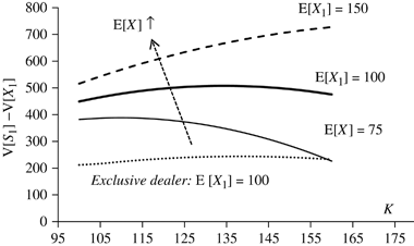
In the plots in Figure 8 we show the variance gap when X ₁ and X ₂ are normally distributed. The sales variance increases as the coefficient of variance of the underlying demand signal increases. Similar to the exclusive dealer case, these results have important implications for the manufacturer. If the demand variability is reduced the variability of observed sales can be regulated. However, the higher sales variance is caused due to the dealer's fluctuating effort to reach the threshold (see Lemma 6).

Figure 8

Impact of Coefficient of Variation on Variance Gap with a Δ‐Contract and Normally Distributed Demand (p=150, g(e)=e ^0.5, Δ=75, and c(e)=0.001e ²)

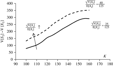
Finally, in this section, we study the effect on sales variance for product 1 when manufacturer 2 offers a higher (lower) marginal payout on reaching the threshold for product 2. Let Δ₁ and Δ₂ denote the marginal payouts of products 1 and 2, respectively. We use the same experimental parameters as before and the demand signals for both the manufacturers are assumed to be normally distributed. Figure 9 shows the results of these numerical experiments, i.e., vs. K for different levels of Δ₂. The solid dark line in Figure 9 corresponds to the base case when Δ₁=Δ₂=75. The dashed curve above corresponds to the case when Δ₂ is increased to 150 and the curve below corresponds to the case when Δ₂ is decreased to 50. As is readily observable, the variance of sales for product 1 is lower when Δ₁>Δ₂. However, the variance of sales continues to be higher than the underlying demand variance . It helps to increase the marginal payout to reduce sales variance but the benefits must be carefully compared against the additional costs incurred. Moreover, the sales variance could also increase for both products if Δ₂ is also increased for product 2 to match the increase Δ₁.

Figure 9

Effect of Different Marginal Contributions (p=150, g(e)=e ^0.5, and c(e)=0.001e ²)

5.1.2. The D‐Contract. In this section we consider the case when each manufacturer offers a D‐contract to the non‐exclusive dealer. We begin by enumerating the possible sales and profit outcomes for the non‐exclusive dealer. In this case there are nine possible sales scenarios. Similar to section 5.1.1, let S _ij=X _i+g(e _ij) represent the sales for product i under scenario j, where e _ij is the effort exerted by the dealer for product i under scenario j. The three sales possibilities for each product are (1) S _ij<K, (2) S _ij=K, or (3) S _ij>K. Consequently there are nine possible sales scenarios. Below, we enumerate the dealer's profit Π_j corresponding to each scenario j=1, …, 9. 17 18 19 20 21 22 23 24 25

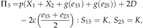
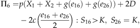
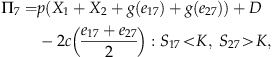
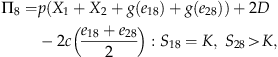
It is noteworthy that each profit function Π_j (j=1, …, 9) is concave in e _1j and e _2j, respectively. We use the first‐order optimality conditions to compute the optimal effort levels that achieve the maximum. We include the complete technical analysis of the D‐contract with a non‐exclusive dealer in the accompanying supporting information appendix (see Appendix S2). In this section, however, we simply summarize our analysis in Lemma 7.

Lemma 7. The optimal efforts exerted for product 1, within the appropriate profit (sales) zones given in equations (17)–(25) , are as follows:

(a)

(b)

, and

(c)

, and such that and for j∈{4, 6}.

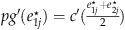
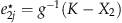
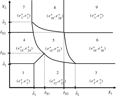
In Lemma 7, c′(·) represents the partial derivative with respect to the appropriate effort and is evaluated at the average value of the optimal efforts. Moreover, it is assumed that the threshold K is suitably large for the optimal effort values to be defined. The results for product 2 are symmetrical. Figure 10 helps us visualize the profit regions and the corresponding optimal effort decisions detailed in Lemma 7. The regions, identified by the bold numbers and demarcated by solid lines, correspond to the index (j=1, …, 9) of the profit function that dominates in that region. Just as in the earlier case with the Δ‐contract, the cutoff values (for regions of X ₁ and X ₂) are nested as follows: . We characterize these cutoff values and the equations for the boundaries between the regions in the supporting information appendix (see Appendix S2). The regions in Figure 10 also correspond to the observed sales. For example, in regions 1, 3, 7, and 9, of Figure 10, the sales are either higher or lower than the threshold K for both products (but never at K.) In regions 2 and 8, the sales for product 1 equal K. In region 5, sales for both products equal the threshold K. Recollect our definition of γ _X in (12). γ _X essentially characterizes the maximum effort exerted by the exclusive dealer to reach the threshold. In contrast, in the case of a non‐exclusive dealer, the nested structure implies that there exists a non‐empty range of demand signals for which the dealer lowers the effort for product 1 below , and raises the effort for product 2 above g ⁻¹(γ _X) to reach K. Essentially, in such situations, the non‐exclusive dealer exerts an effort level higher than the maximum effort an exclusive dealer would exert. Consequently, the non‐exclusive dealer's expected profit is strictly greater than the sum of expected profits of two exclusive dealers with a D‐contract. We prove this in the supporting information appendix (Appendix S2).

Figure 10

The Optimal Effort Levels for a D‐Contract

It is difficult to analytically infer if a positive bonus, D, has a favorable impact on the reduction of sales variance for individual products (it depends on the probability distributions of the underlying demand signals). Next, we analyze the impact on sales variance through numerical experiments.

5.1.3. Numerical Study for the D‐Contract. We begin by studying the case when the demand signals for both the manufacturers are normally distributed with a mean of 150 and a standard deviation of 30. The parameters of the experiments are as follows: p=500, g(e)=e ^0.5, D=10,000, and c(e)=0.001e ². It is worth noting that using these parameters the cutoffs at any threshold level K are and 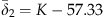. The optimal effort and δ _X2=K−50. Figure 11 shows the variance of sales for product 1 as the threshold K is increased from 110 to 170 in steps of 10. Note that the sales variance is lower than that of the demand signal X ₁ until . This is similar to the exclusive dealer case. However, for larger values of K (compared with ), the sales variance could be larger than (see Figure 12). This suggests that, unlike the case with a Δ‐contract, the manufacturer is able to regulate her sales variance with a D‐contract provided the threshold parameter is chosen appropriately. By appropriately we mean linking the threshold to the underlying demand distribution.

Figure 11

The Observed Sales Variance for Different Levels of K—Normal Distribution (p=150, g(e)=e ^0.5, D=10,000, and c(e)=0.001e ²)

Figure 12

The Observed Sales Variance for Different Levels of K—Uniform Distribution (p=500, g(e)=e ^0.5, D=10,000, and c(e)=0.001e ²)

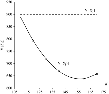
Next, using the same experimental parameters, we study the case when the demand signals are uniformly distributed between 0 and 200. Figure 12 shows the plots for for these experiments. The plots with a uniform distribution confirm our earlier observation when the demand signal follows a normal distribution. Both the sets of numerical experiments suggest that when the demand signals are independent and identically distributed an appropriately designed D‐contract may be able to regulate the sales variance better.

It is noteworthy, however, that the when threshold level is not designed appropriately (based on the underlying demand distribution) the sales variance can be higher even with a D‐contract. To illustrate this, we consider the case when X ₁ is consistently low when compared with X ₂, i.e., the mean and variance of X ₁ is lower than that of X ₂. However, both the manufacturers offer identical threshold incentives. Specifically, we consider the case when . The experimental parameters are similar to the uniform distribution case studied earlier. The results of these experiments are plotted in Figure 13. Note that as K increases also increases (see the supporting information Appendix S2 for details). We randomly draw X ₁ from a uniform distribution between 0 and . Consequently, since changes the variance of the underlying demand signal X ₁ also changes. In Figure 13, we plot the and for different levels of K (and ). As can be observed the sales variance is consistently higher than that of the underlying demand signal. This experiment demonstrates that by not choosing the threshold level appropriately the manufacturer is unable to regulate the sales variance with D‐contract and loses both due to lower expected sales and higher sales (order) variance.

Figure 13

The Observed Sales Variance for Different Levels of K when (p=500, g(e)=e ^0.5, D=10,000, and c(e)=0.001e ²)

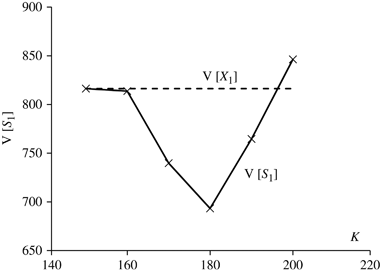
5.2. Products with Different Demand Distributions

Building on our previous example, in this section, we consider the case when the underlying demand signals are not identical. More specifically, we consider the case when the variances of the underlying demand signals are different for X ₁ and X ₂. For these experiments, we focus on the D‐contract because we have already shown that the variance is always higher than the underlying demand variance with a Δ‐contract. Our goal is to test if the variance of sales continues to be lower than when the demand distributions are different. Figure 14 illustrates the results of these experiments. We plot the variance of sales at different levels of the threshold K. The experimental parameters are same as before except with X ₁ being distributed normally with a mean of 150 and a standard deviation of 30. X ₂ was also assumed to be normally distributed with a mean of 150. The case when is used as the benchmark case, and is indicated by the solid dark line in Figure 14. As is readily observable, when is decreased to 100, the variance of sales observed for product 1, , increases. On the other hand, when is increased to 2500 increases further. In all the cases, however, is strictly below for thresholds K=150, …, 190. These numerical experiments suggest that product 1 benefits by reduction in sales variance when the demand variance of the competing product (product 2) increases, i.e., decreases as increases. These results do not change even if we use different means for the distributions or use different distributions (e.g., uniform and normal) for each of the products.

Figure 14

The Observed Sales Variance for Different Levels of K when (p=500, g(e)=e ^0.5, D=10,000, and c(e)=0.001e ²)

6. Discussion

Firms offering incentive schemes typically do so to achieve certain objectives, for example, increase expected profits or sales. However, sometimes such incentives result in undesirable, and unforseen, effects that could hurt the operational efficiency of the firm. In this paper, we analyze the impact of threshold‐based incentives on a manufacturer's sales variability.

In the case of an exclusive dealership we show that the manufacturer is able to regulate the sales variance better with a bonus contract. Our study of threshold‐based incentives for non‐exclusive dealers shows two main results. The first is that, with a Δ‐contract, non‐exclusivity of dealers increases the sales variance observed by the manufacturers. Even though the dealer observes a lower sales variance, in terms of aggregate sales, than an exclusive dealer, the variance of sales observed by each manufacturer goes up. Our second result is that the D‐contract continues to perform better on this dimension for appropriately chosen threshold values. The numerical analysis with asymmetric distributions also suggests that the performance of the D‐contract is reasonably robust. However, even with a D‐contract, the incentive provider must choose the threshold K appropriately, i.e., it must be consistent with the actual demand distribution. Otherwise, the sales variance can be higher than the underlying demand distribution for a D‐contract as well. Essentially, in such a case, the dealer chooses to shift effort toward the higher demand product and consequently the product (manufacturer), with a consistently lower demand compared with the threshold level, observes a higher sales variance even under a D‐contract.

The implications for the manufacturer are twofold. First, we observe that the gap between the sales variance and the underlying demand variance increases as the coefficient of variation of the demand increases. This suggests that the incentive provider could potentially regulate the observed sales variance better if she invests some effort in smoothing the underlying demand. One possible way to achieve this is by better information sharing between members of the supply chain. Second, the manufacturer should carefully design her threshold incentive parameters. Specifically, the choice of the threshold level is important in controlling the observed sales variance. One possible way is to link the threshold level to the underlying demand signal by carefully choosing correlated economic indicators or market signals. Sohoni et al. (2010) discuss such a scheme for multi‐period threshold‐based contracts.

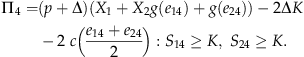
Recollect Chrysler's incentive scheme described in section 1. On careful observation it is evident that this plan is a combination of the two forms of contracts studied in this paper, i.e., a (p, Δ, D, K) contract. In this instance D=ΔK and the dealer receives the additional marginal payment of Δ only on reaching and surpassing the sales threshold K. In response to this incentive scheme, several Chrysler dealers complained (Wernle 2006) that the sales targets were not based on market demand but “on the amount of cars Chrysler had jammed down the regional business center's throat.” In this case Chrysler dealers were complaining that threshold levels were too high and the incentive was not designed to elicit higher sales effort given the depressed market conditions. Such anecdotal evidence suggests that a manufacturer should choose a threshold level that aligns the dealer's sales effort appropriately given the market conditions. The company found that, when the dealers realized they could not reach their monthly goals, their sales efforts plummeted. This could be one of the plausible reasons why Chrysler sales cycled through booms and busts. Dealers would order fewer cars during months in which they felt they could not reach the incentive threshold, but more cars during months where they felt they could. Consequently, there was an increase in the variability of sales, as well as increased production and inventory costs, which eroded profits for the auto‐manufacturer. Eventually Chrysler decided to ease the incentive scheme (Wernle 2006).

Finally, we would like to comment about moving to a constant‐margin contract (without any threshold levels) if regulating sales variance is critical. It is possible to construct a constant‐margin contract such that the dealer's expected profit is at least as large as that under a Δ‐contract (see the supporting information Appendix S3). Because the effort exerted in this case is constant, the sales variance for a constant‐margin contract is the same as that of the underlying demand signal. The manufacturer can thus regulate the sales variance better. There is anecdotal evidence suggesting that some firms have done this in the past. For example, Ford (Wilson 2006) has shifted to constant‐margin contracts for some of its products. Overall our analysis indicates that manufacturers should carefully design threshold‐based incentives to induce higher dealer effort, especially if they have a high cost associated with sales variance.

This research can be extended in multiple directions. Some of the limitations of our model are that demand is stationary and there are no autocorrelated demand processes or varying threshold values. Our model implicitly assumes a multi‐period infinite horizon model with no learning between periods, i.e., the manufacturer does not learn about the nature of the impact of the dealer's effort function and cannot observe X or any other correlated signal in the economy to estimate X. Furthermore, in the current setting we consider a manufacturer selling through a single dealer. We assume that the manufacturer is not capacitated. It is plausible that in a capacitated system the sales variance would be dampened. However, the analysis in this paper provides an upper bound on the magnitude. Another important issue not considered in our setting is the presence of multiple dealers and the ensuing competition. This will change the nature of the analysis. Dealer competition may affect the nature of the optimal effort exerted by the dealer. Additionally, in our setting we have ignored issues related to inventory and lead‐time. These considerations will make the analysis technically very challenging but can provide avenues for future research.

Footnotes

Appendix

Acknowledgments

The second author's research is supported by NSF Grant number DMI‐0457503. We thank Martin A. Lariviere and Achal Bassamboo for valuable comments on the paper.

¹We use the terms threshold and quota interchangeably throughout this paper.

²A dealer got no additional cash for sales below 75% of the sales target, US$150 per vehicle for sales between 75.1% and 99.9% of the sales target, US$250 per vehicle for sales between 100% and 109.9%, and US$500 per vehicle for reaching 110% of the sales target.

³We show the similarity in .

References

Basu

Rajiv

Srinivasan

Staelin

. 1985. Salesforce compensation plans: An agency theoretic perspective. Mark. Sci. 4 (4): 267–291.

Chen

2000. Sales‐force incentives and inventory management. Manuf. Serv. Oper. Manage. 2 (2): 186–202.

Chen

2005. Salesforce incentives, market information, and production/inventory planning. Manage. Sci. 51 (1): 60–75.

Coughlan

A. T.

1993. Handbooks in OR & MS, Chapter 13. Elsevier Science Publishers B. V., Amsterdam, 611–651.

Coughlan

A. T.

Subrata

S. K.

. 1989. Salesforce compensation: Theory and managerial implications. Mark. Sci. 8 (4): 324–342.

Gonik

1978. Tie saleman's bonuses to forecasts Harvard Business Review, March‐June 116–123.

Harris

Raviv

. 1979. Optimal incentive contracts with imperfect information. J. Econ. Theory 20: 231–259.

Holmström

1979. Moral hazard and observability. Bell J. Econ. 10 (1): 74–91.

Horn

1979. Some inequalities for the expectation of a product of functions of a random variable and for the multivariate distribution function at a random point. Biometrical J. 21 (3): 243–245.

10.

Joseph

Kalwani

. 1998. The role of bonus pay in salesforce compensation plans. Ind. Mark. Manage. 27: 147–159.

11.

Kim

S. K.

1997. Limited liability and bonus contracts. J. Econ. Manage. Strategy 6 (4): 899–913.

12.

Lal

Srinivasan

. 1993. Compensation plans for single‐ and multi‐product salesforces: An application of the Holmstrom–Milgrom model. Manage. Sci. 39 (7): 777–793.

13.

Lal

Staelin

. 1986. Salesforce compensation plans in environments with asymmetric information. Mark. Sci. 5 (3): 179–198.

14.

Lee

H. L.

Padmanabhan

Whang

. 1997. The bullwhip effect in supply chains. Sloan Manage. Rev. 38 (3): 93–102.

15.

Lee

H. L.

Tang

C. S.

. 1996. Modelling the costs and benefits of delayed product differentiation. Manage. Sci. 43 (1): 40–53.

16.

Lee

H. L.

Tang

C. S.

. 1998. Variability reduction through operations reversal. Manage. Sci. 44 (2): 162–172.

17.

Oyer

2000. A theory of sales quotas with limited liability and rent sharing. J. Labor Econ. 18 (3): 405–426.

18.

Post‐Distpatch

St. L.

2001. Chrysler eases unpopular dealer subsidy program blamed for poor sales New York Times, Business, December 9, p. F7.

19.

Raju

J. S.

Srinivasan

. 1996. Quota‐based compensation plans for multiterritory heterogeneous salesforces. Manage. Sci. 42 (10): 1454–1462.

20.

Sappington

1983. Limited liability contracts between principal and agent. J. Econ. Theory 29: 1–21.

21.

Sinha

Zoltners

A. A.

. 2001. Sales‐force decision models: Insights from 25 years of implementation. Interfaces 31 (3): S8–S44.

22.

Sohoni

Bassamboo

Chopra

Mohan

Sendil

. 2010. Threshold incentives over multiple periods and the sales hockeystick phenomenon. Res. Log. (NRL)57: 508–518.

23.

Wernle

2006. Chrysler to ease dealer quotas. Available athttp://www.autonews.com/apps/pbcs.dll/article?AID=/20061225/SUB/61221077/1078/SUBrefsect=DEALERStemplate=printart(accessed date September 10, 2010).

24.

Wilson

2006. Ford lowers bar on bonus for dealers. Available athttp://www.autonews.com/apps/pbcs.dll/article?AID=/20060109/SUB/60106055/1023refcat=template=printart(accessed date September 10, 2010).

25.

Xiao

2007. Saleforce incentives: Matching supply and demand under information asymmetry. Ph.D. thesis. Available athttp://www.proquest.com(accessed date June 2009).

26.

Zoltners

A. A.

Sinha

Lorimer

S. E.

. 2006. The Complete Guide to Sales Force Incentive Compensation. AMACOM, New York.