Distribution Planning to Optimize Profits in the Motion Picture Industry

Abstract

We consider the distribution planning problem in the motion picture industry. This problem involves forecasting theater‐level box office revenues for a given movie and using these forecasts to choose the best locations to screen a movie. We first develop a method that predicts theater‐level box office revenues over time for a given movie as a function of movie attributes and theater characteristics. These estimates are then used by the distributor to choose where to screen the movie. The distributor's location selection problem is modeled as an integer programming‐based optimization model that chooses the location of theaters in order to optimize profits. We tested our methods on realistic box office data and show that it has the potential to significantly improve the distributor's profits. We also develop some insights into why our methods outperform existing practice, which are crucial to their successful practical implementation.

Keywords

motion picture industry forecasting distribution planning theater selection optimization

1. Introduction

The motion picture industry is an important sector of the US economy. Movie releases at theaters generated approximately US$9 billion in revenue in 2005, representing a nearly 20% increase since the beginning of the decade. In spite of this increase, the Motion Picture Association of America (MPAA) reports that only nine of the 549 movies released in 2005 generated profit higher than US$50 million (http://www.mpaa.org). The average cost of a studio‐released movie was nearly US$96 million in 2005, up from US$54.1 million in 1995. The major component of this cost was the development and production budget, which averaged around US$60 million in 2005, followed by marketing (US$36 million), and distribution costs. Depending on the distribution strategy chosen by the movie distributor (e.g., platforming, wide, or saturation release), distribution costs can be up to US$9 million and averaged around US$3.83 million per movie in 2005. While distribution represents a smaller portion of a movie's total investment in comparison to development, production, and marketing costs, effective distribution is critical to box office success and ultimate financial return from a movie (Reardon 1992, Thomas 1998).

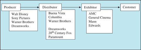
Distribution of a motion picture is handled by its distributor, who forms an important link in the motion picture industry supply chain (Figure 1). Examples of major distributors in the motion picture industry include Buena Vista (Walt Disney's distribution arm), Columbia (Sony's distribution arm), Universal, Paramount, Fox, and Warner Brothers. The motion picture distribution industry is highly concentrated with these six distributors accounting for 70% of box office sales in the United States. The distributor secures rights from the producer, undertakes marketing (including advertising in television, local, and national media) and has to choose at which theaters to screen the movie. The theaters are owned by exhibitors such as AMC, Regal, General Cinema, and Mann. Historically, distributors have been more dominant and profitable than exhibitors in the motion picture industry. To achieve balance of power between these entities, there has been federal regulation and individual statutes passed by states. The aims of these statutes were to ensure that distributors picked exhibitors on a movie by movie basis using a competitive bidding process. A detailed overview of the history of anti‐trust legislation in the motion picture industry can be found in Vany and Eckert (1991). However, with increasing overcapacity of screens and changes in technology that enables different channels of distribution such as DVD's, satellite, and the Internet, the balance of power is again being shifted in favor of the distributors. Scott (2005) provides a comprehensive discussion of these issues.

Figure 1

The Motion Picture Industry Supply Chain

Distribution planning for a new movie is done far in advance of the actual release date. The studio (i.e., producer) announces the distributor several months before actual theatrical release of the movie. Then, the distributor solicits bids to exhibit the movie. In response, exhibitors contact the distributor with bids to screen the movie. These bids include a proposed set of theaters and their coverage territory, initial duration of play, and revenue‐sharing agreements. The distributor now needs to choose which exhibitors and theaters to use for the initial screening of the movie. This decision has to be made at least 3 months before the scheduled theatrical release of the movie. These decisions are then conveyed to the exhibitor. If the distributor picks a particular theater, this movie is scheduled to be shown there for the agreed period. If not, the exhibitor has the option to try other movies, as this planning takes place far in advance of when the movie is actually released in the theater. As the initial duration of play for the selected theaters expires (which is agreed by the contract), the distributor is free to add additional theaters as offers to show new movies are made by the exhibitors (McGrath 2004, Rothenberg 2003).

The distribution planning problem involves forecasting theater‐level box office revenues for a given movie and using these forecasts to choose the best locations to screen a movie. Distribution planning in the motion picture industry is made difficult by a complex environment. Forecasting box offices revenues for a given duration is challenging as movies are experiential products (Hirschman and Holbrook 1982) and, consequently, it is difficult to forecast their audience appeal until they are already available in the theaters. This is because audience appeal varies widely depending on movie attributes such as genre, star presence, special effects, MPAA ratings, critical reviews, etc. Even experienced analysts in the industry have not been very successful in forecasting box office revenues (Table 1). While there has been some academic research on aggregate box office forecasting, disaggregate theater‐level forecasting is even harder due to dissimilarity in location‐specific characteristics of theaters, such as amenities and demographics (i.e., median income, age, population density, etc.). This causes significant differences in revenue for the same movie in different markets (Table 2). All these factors conspire to make the theater‐level box office revenue forecasting problem in the motion picture industry an extremely challenging problem. Even after the forecasts are generated, picking the optimal location of theaters to show a particular movie is a challenging problem due to the large number of movies released each year by multiple distributors and the abundance in potential theater locations. For example, there were 500 movies released in the year 2005 and more than 7000 possible theater locations in the United States and Canada to show these movies.

Table 1

Examples of Missed Box Office Forecasts

Title	NRG estimate^* (US$ in million)	Actual box office (US$ in million)	Relative percentage error^† (%)
X‐Men	29.5	54.5	−45.9
The Mummy Returns	50	70.1	−28.7
Charlie's Angels	28	40.1	−30.2
The Perfect Storm	21.5	41.3	−47.9
Chicken Run	9	17.5	−48.6
The Patriot	25	22.4	+11.6
The Story of Us	18	9.7	+8.6
Fight Club	14	11	+27.3
Titan A. E.	12.5	9.4	+33
Star Wars: Episode I.	150	105.7	+41.9

National Research Group's estimate of the opening weekend box office.

^†

Relative percentage error=(NRG estimate−Actual BO)/Actual BO.

Source: IMDB and Variety Magazine.

Table 2

Box Office Revenues at Selected Markets

Markets^*	The Matrix Reloaded (US$)	Star Wars: Episode II (US$)
Boston	38,371	35,829
Cleveland	21,105	21,559
Dallas	31,207	35,385
Denver	31,423	28,663
New York	36,968	53,499
Pittsburgh	23,193	18,683
San Francisco	60,336	60,169
St. Louis	22,813	23,410
Tampa	25,043	25,763

Movies are shown in the same number of theaters in each market and revenues reported are Friday to Sunday averages over duration of play.

Data Source: Nielsen EDI's box office sample.

Despite the practical relevance and complexity of this problem, we have found nothing in the academic or managerial literature that describes how to conduct effective distribution planning in the motion picture industry. This paper presents a method for addressing these issues and addresses an important problem in entertainment operations management, an underrepresented area in the growing stream of research in service operations management (Apte et al. 2008, Spohrer and Maglio 2008). Specifically, we have developed an empirical technique that provides a box office revenue estimate over time for a new motion picture at a selected theater. We use these estimates to model the distributor's location selection problem (DLSP) as an integer programming model. This model chooses the location of theaters to screen the movie in order to optimize the distributor's profits. We have tested our methods on actual industry data and show that our approach offers the potential to significantly improve box office profits for new movies.

This paper is organized as follows. In section 2, we review the relevant literature. In section 3, we develop an empirical method to estimate the theater‐level box office revenue for a given movie. In section 4, we formulate the DLSP. We develop heuristics to solve this problem and also construct upper bounds to evaluate the quality of these heuristics. We present computational results in section 5. We use these results to assess the performance of our forecasting method and the heuristics to solve the DLSP. These results also provide insight into what affects theater‐level box office revenue and the impact of these revenue estimates on the location choice decision. In section 6, we test our methods on realistic box office data and show that it has the potential to significantly improve current industry practice. In the concluding section, we summarize our work and present future research directions.

2. Literature Review

There is extensive literature on motion pictures in the popular press and in the film and television areas (Bart 2000, Hayes and Bing 2004, Vogel 2001); however, much of this is descriptive in nature and relies heavily on anecdotal industry knowledge. There is a limited, but emerging, stream of academic research focused on the motion picture industry. Eliashberg et al. (2006) provide a comprehensive overview on the critical issues in practice, current research, and future research directions in the motion picture industry. Areas of research include product diffusion (Elberse and Eliashberg 2003, Neelamegham and Chintagunta 1999), seasonal release patterns (Einav 2002, Krider and Weinberg 1998), ancillary markets (Lehmann and Weinberg 2000), and contract design and competition (De Vany and Walls 1996). In the broader context of the entertainment industry, there has been work on scheduling commercial videotapes (Bollapragada et al. 2004), managing on‐air advertisement inventory (Bollapragada and Mallik 2008), media revenue management (Araman and Popescu 2009), and theme park flow management (Rajaram and Ahmadi 2003).

There has been a significant stream of research on aggregate box office forecasting of new motion pictures. Many previous studies have attempted to explain aggregate box office success as a function of movie attributes such as budget, star power, MPAA rating, release timing, and Academy Award nominations and winners (Litman and Ahn 1998, Wyatt 1994). Recent work focuses on the influence of a major distributor (Sochay 1994), advertising and critical reviews on box office success (Eliashberg and Shugan 1997, Zuckerman and Kim 2003, Zufryden 1996). Sawhney and Eliashberg (1996) develop a parsimonious aggregate forecasting model and test it on realistic data. However, none of this work considers disaggregated theater‐level box office revenue forecasts for a new movie. There have been several papers on scheduling of screens with multiple movies (Eliashberg et al. 2009, Dawande et al. 2010, Swami et al. 1999). This is an important tactical problem once the location of the theater to screen a movie is chosen, but these papers do not consider the broader strategic question on which theaters to show the movie, as addressed in DLSP.

This paper makes the following contributions. First, we develop a method to calculate detailed disaggregated theater‐level box office sales forecasts, based on both movie attributes and theater characteristics. Second, unlike the work discussed above, we directly consider the DLSP. Correct selection of theater location is essential to the ultimate box office success of a movie and we develop an optimization model to make this choice. Third, we test this model extensively on realistic data and show that it has the potential to significantly improve existing industry practice.

3. Forecasting Theater‐Level Box Office Revenues

Consider a distributor who has to make box office revenue forecasts at each of the possible theaters where they could release a new movie. To provide a precise statement of this problem, we consider n possible theaters and let j∈N=(1, …, n) index the set of theaters. Let π _ijt define the expected box office revenue forecast when movie i is shown at theater j in week t, where i∈M=(1, …, m) indexes the set of movies and t∈Q=(1, …, q) indexes the set of time periods. Estimating π _ijt is critical for several reasons. First, when we tabulate total box office revenue across theaters over time (i.e., , ∀t), we obtain the adoption pattern for movie i. This pattern provides crucial guidance for various strategic decisions made by the distributor such as determining the marketing budget and eventually the distribution strategy (i.e., platforming, wide, or saturation release) for the movie. This, in turn, is used in determining the maximum number of theaters across regions, the minimum play length at any theater, and, finally, in negotiating the revenue‐sharing contract during and after this minimum play length. Second, π _ijt is a key parameter in determining at which theaters the movie will be screened and, ultimately, its box office success.

However, estimating π _ijt is challenging for several reasons. First, it is difficult to understand which movie attributes and theater characteristics will affect theater‐level box office revenue and how they do so. Second, it is challenging to estimate how this complex relationship between theater characteristics, movie attributes, and box office revenues changes over time. Finally, this estimation is difficult, as forecasting box office revenues requires an understanding of the individual moviegoer's decision process to see a given movie and incorporating this process into the estimation method.

Typical industry practice when forecasting box office revenues is to compare a new movie with recently released movies that are similar in one movie attribute and use multiple, separate comparisons to study the effect of different movie attributes on box office revenues (Rothenberg 2003, Tannenbaum 2001). In addition, some distributors also use multiple regression analyses on a set of comparable attributes. While these procedures are simple and provide flexibility to incorporate subjective expertise, they are not very accurate. This is because this approach does not explicitly consider any of the above‐discussed aspects that make estimating π _ijt an immensely challenging problem. There are box office estimation models in the academic literature that incorporate some of these aspects. Most of these models run multiple regressions directly on box office revenue as a function of certain sets of movie attributes (Litman and Ahn 1998). A major limitation of this method is that it only provides point estimates for box office revenues by assuming an unrestricted horizon for exhibiting the movie. In addition, this approach does not consider significant variations in box office revenues across time periods and differences in adoption patterns across movies. Sawhney and Eliashberg (1996) developed a parsimonious model to forecast a movie's box office success as a function of time. They use an innovative method that incorporates an individual moviegoer's decision process to adopt (or see) a given movie and also consider the impact of different movie adoption patterns. However, the objective of this model is to estimate box office revenue at the national or aggregate level, and this approach cannot be used to provide local or disaggregate location‐specific, theater‐level estimates.

To overcome the described challenges inherent in estimating π _ijt, we develop a four‐step method. These steps are outlined in Figure 2. In Step 1, we extend the Sawhney and Eliashberg (1996) model to include location‐specific, theater‐level characteristics. We estimate the parameters of this model using nonlinear regression on a historical database of realized box office revenues for selected movies. In Step 2, we use multiple regression models to link the estimated model parameters to movie attributes and theater characteristics corresponding to this historical database; then, we also consider any potential interactions between these variables. This step provides us with a function that estimates model parameters given a set of movie attributes and theater specific characteristics. In Step 3, we use this function to estimate the model parameters for a new movie given its attributes and the location‐specific characteristics of the theater under consideration. In Step 4, we use these estimates of the model parameters of Step 1 to estimate the box office revenue for the new movie at a given theater across time. Below, we describe each of these steps in detail.

Figure 2

Methodology for Estimation of π _ijt: Theater‐Level Box Office Revenues for a New Movie

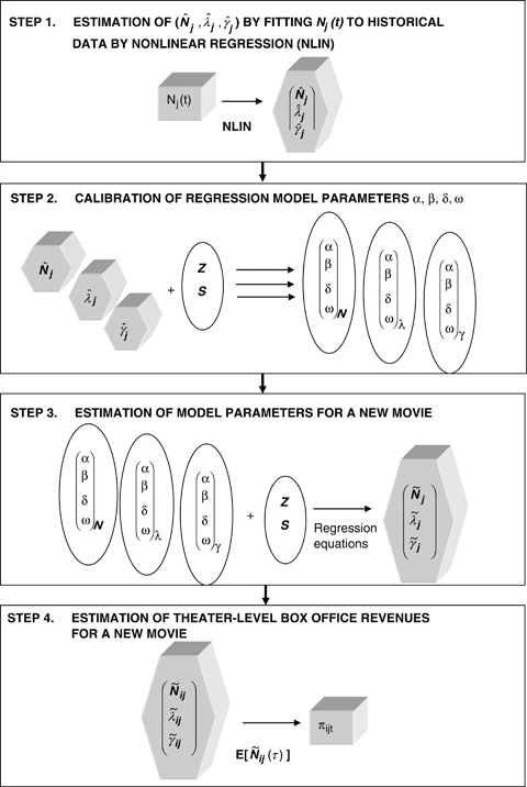
Step 1: Incorporation of theater‐level characteristics

In this step, we extend the Sawhney and Eliashberg (1996) model to include location‐specific, theater‐level characteristics. Here, we assume that an individual movie patron's decision process to choose whether to watch a movie depends on two independent sub‐processes: (1) the decision to see a movie p in theater j, followed by (2), the decision to visit theater j. These processes are modeled as stochastic processes with stationary parameters λ _pj representing the time‐to‐decide parameter and γ _pj representing the time‐to‐act parameter. Then, the expected time to decide becomes (1/λ _pj) and the expected time to act becomes (1/γ _pj). Although it is plausible that the time‐to‐decide process is mainly influenced by movie attributes, we believe that the availability of the chosen movie in a theater that is acceptable to the patron also affects the time‐to‐decide parameter. Once the individual has decided to watch a movie, the next decision is where to watch it, which is again influenced by theater characteristics.

Following the approach of Sawhney and Eliashberg (1996), the expected cumulative number of adopters of movie p at theater j by time τ can then be expressed as 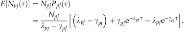1 where N _pj(τ) is the distribution of the cumulative number of adopters of movie p at theater j by time τ approximated using binomial distribution, N _pj is the maximum potential market size in the vicinity of theater j, and P _pj(τ) is the cumulative density function of the event when an individual decides to see movie p in theater j and acts on the decision by time τ. We estimate parameters N _pj, λ _pj, γ _pj by using nonlinear regression to fit (1) to historical data of theater‐level box office revenues over time across a range of w movies at all the required theaters and let p∈H=(1, …, w) index these movies with historical data.

Step 2: Calibration of regression model parameters from historical box office information

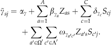
The second step in the estimation process is to connect the estimated value of parameters , ∀j∈N, ∀p∈H from Step 1 to movie attributes, theater characteristics, and their possible interactions. To do this, we rely on multiple regressions based on the historical box office information ∀p∈H used in Step 1.

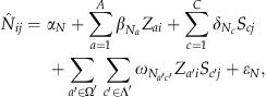
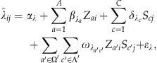
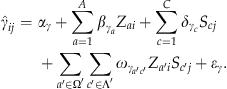
Let Z _i=(Z _1i, …, Z _Ai) define the movie attribute vector for movie i. Here, movie attributes include aspects such as genre, star presence, special effects, MPAA ratings, critical reviews, etc. To incorporate theater characteristics, let S _j =(S _1j, …, S _Cj) define the vector of theater characteristics for theater j. These include location‐specific characteristics of theaters such as amenities and theater size, and demographics factors such as median income, age, population density, etc. Then, the multiple regression equations to estimate the regression coefficients are 2 3 4

Here, α _N, α, and α denote the population intercepts and , , and (a∈Ω=(1, …, A), and , , and (c∈Λ=(1, …, C) represent the regression coefficients associated with vectors Z and S , respectively. In addition, the interaction terms associated with regression coefficients are , , and , where a′∈Ω′⊆Ω and c′∈Λ′⊆Λ. Finally, ɛ _N, ɛ, and ɛ are independent and identically distributed random error terms.

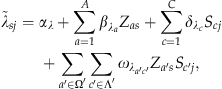
Step 3: Estimation of model parameters for a new movie

Let represent the model parameters for a new movie s in theater j. Once the regression coefficients of Equations (2) through (4) are calculated, we use the known attributes Z _s=(Z _1s, … Z _As) of new movie s and individual theater characteristics at theater j to estimate parameters , and as 5 6 7

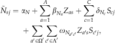
Step 4: Estimation of theater‐level box office revenues for a new movie

In this step, we use the estimates of , and from (5) to (7) in (1) to estimate , the expected cumulative number of adopters for new movie i at theater j until time τ, as 8

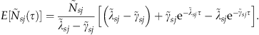
Let φ _j be the ticket price at theater j and t=τ ₂−τ ₁ be the time interval under consideration. Then, we calculate π _sjt as 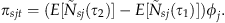9

In section 5, we conduct computational experiments to test the accuracy of this method.

4. The DLSP

Once we forecast theater‐level box office revenues, the distributor needs to use this forecast to choose at which theaters to show a new movie, in order to maximize profits. To address this problem, we consider n possible theaters and let j, j′∈N=(1, …, n) index the set of theaters. These movie theaters are located in r regions indexed by r∈P=(1, …, u).

Define the variables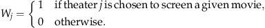

We are given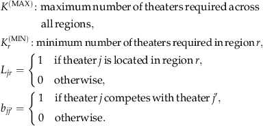

Here, parameter K ^(MAX) is defined by the type of distribution strategy (i.e., limited, platforming, wide, or saturation release) chosen for the particular movie. The distribution strategy is chosen to be consistent with the marketing budget for a given movie. Next, the regions chosen are often major metropolitan areas. The minimum number of theaters per region is often specified by past experience. Finally, parameters are derived from the coverage territory specified by the exhibitor in each territory. The coverage territory is defined by a set of competing theaters that need to be excluded in each territory, which in turn specifies .

Recollect that π _ijt defines the expected box office revenue forecast when movie i is shown at theater j in week t, where i∈M=(1, …, m) indexes the set of movies and t∈Q=(1, …, q) indexes the set of time periods. Let t _ij∈Q denote the duration chosen by the exhibitor to show movie i at theater j. Note that t _ij can be optimally chosen using the models described in Swami et al. (1999, 2001) or Somlo (2005) and is affected by the minimum play length P ^(MIN) fixed by a contractual agreement between the distributor and exhibitor. Then, the distributor's expected box office profit during this period is given by 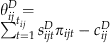, where c _ij ^D is the distribution cost of movie i to theater j, and constant s _ijt ^D represents the portion of revenues allocated to the distributor for movie i at theater j during week t. This factor depends on the duration chosen by the exhibitor and the nature of the contractual agreement between the exhibitor and distributor.

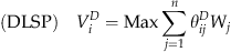
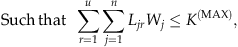
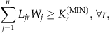
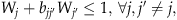
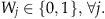
The DLSP can be represented by the following binary integer program: 10 11 12 13 14

Objective function (10) is chosen to maximize the distributor's total expected box office profits for movie i by the appropriate choice of theaters. Constraint (11) ensures that the total number of theaters selected to screen a movie does not exceed K ^(MAX). Constraints (12) guarantee that a set minimum number of theaters are picked for each region. Constraints (13) ensure that the distributor does not pick competing theaters. This is important because a distributor often chooses multiple exhibitors to show a movie. Consequently, to prevent dilution of sales at the selected theater, exhibitors require that competing theaters within the vicinity are not picked. Finally, 0–1 integrality of the variables is imposed by constraints (14).

The DLSP can be used by the distributor to determine the optimal set of theaters for the initial screening of a movie. As the minimum play length commitment for the theaters expires, the distributor is free to add additional theaters as new offers to show the movie are made by exhibitors. In this case, the distributor would need to consider the set of theaters in which the movie still has to be shown, reduce K _r ^(MIN)at the appropriate regions, reduce K ^(MAX) by the total number of theaters where the movie is still being shown, remove the additional theaters for which constraint (13) will not be feasible, and resolve the DLSP. Note that this approach also can be used to include preferred theaters in the beginning or in later iterations of the DLSP. Here, the preferred theaters are akin to the theaters where the movie still has to be shown. Such preferred theaters may be necessary to maintain a long‐term relationship with the exhibitor. Also note that this model can be extended to multiple movies. Here, we would first need to index the parameters and variables of the DLSP by movie index i. Then, the objective function for the DLSP for multiple movies would now be and we would have constraints (11) through (14) for each movie i. Since this problem is decomposable by movie or index i, we could use the same solution procedure to solve the DLSP with a single movie.

Proposition 1. The DLSP is NP‐complete.

Proof. The maximum weighted independent set problem can be derived as a special instance of the DLSP by setting the coefficients L _jr, ∀j, r to 0. As it is known that the weighted independent problem is NP‐complete (Garey and Johnson 2000), this reduction establishes that the DLSP is NP‐complete. ▪

In light of Proposition 1, it is unlikely that we could solve large, realistic problems to optimality. In particular, we found in our computational analysis that we could not find solutions using leading commercial software tools such as the XPRESS and CPLEX solvers in GAMS (Brooke et al. 1992) when the number of theaters is large (over 1800 theaters) and when each theater has many competing theaters (averaging over seven per theater). Consequently, we elected to develop heuristics to solve such instances of this problem. We also present upper bounds to evaluate the quality of these heuristics.

4.1. Upper Bounds

To develop upper bounds on the DLSP, one could relax one or more of constraints (11) through (13) by introducing Lagrange multipliers and solving the resulting sub‐problem optimally. Then, this sub‐problem can be optimized over the multipliers to provide a tight upper bound. However, the upper bound from any such relaxation would be no smaller than a simple linear programming relaxation of the DLSP, in which we relax constraint (14) by allowing W _j∈[0, 1], ∀j. This is because relaxations of the DLSP involving constraints (11) through (13) have the integrality property (Geoffrion 1974), as established by the following proposition.

Proposition 2. Relaxations of the DLSP involving constraints (11) through (13) possess the integrality property.

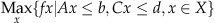Proof. We can represent the DLSP in a generalized matrix form as , where A, b, C, d, and f are the appropriate matrices, Ax≤b represents the set of constraints we keep, Cx≤d represents the set of constraints we relax, and x∈X represents the integrality constraints. Let Co{xɛX|Cx≤d} represent the convex hull formed by the constraints we relax. Since in the DLSP K _r ^(MIN), K ^(MAX)∈N ⁺, ∀r and L _jr, b _jj′∈{0, 1}, ∀r, j, j′ note that Co{x∈X|Cx≤d}={x|Cx≤d} for any relaxation involving constraints (11), (12), and (13). It follows from Geoffrion (1974) that any relaxation of the DLSP involving these constraints has the integrality property. ▪

In light of Proposition 2, we generate an upper bound for the DLSP by solving its linear programming relaxation with W _j∈[0, 1], ∀j.

4.2. Heuristics

In general, the solution provided by the upper bounds may not be feasible for the DLSP due to the violation of the integrality constraints (14). To achieve feasibility, we develop the following heuristics.

4.2.1. The Myopic Heuristic. In the myopic heuristic, we select theaters by first ignoring constraints (13) and optimally solving the resulting problem. Then, we develop an interchange procedure that is aimed at satisfying constraints (13). Recollect that K _r ^(MIN) represents the minimum number of theaters required in region r, K ^(MAX) is the maximum number of theaters across all regions, and θ _ij ^D is the distributor's expected box office profit for movie i at theater j. This heuristic is formalized in the following steps.

Step 1: In each region, select K _r ^(MIN) theaters in descending order of θ _ij ^D. This satisfies constraints (12). Remove the selected theaters from consideration. Sort all of the remaining theaters in descending order of θ _ij ^D and pick an additional theaters. Thus, constraint (11) is binding.

Step 2: We consider the theaters selected by Step 1 and look for those theaters that violate constraints (13). We first remove the violating theater with the lowest θ _ij ^D. We then find a replacement theater that has the highest possible θ _ij ^D without violating constraints (13). This procedure is repeated until all violating theaters across all regions are eliminated.

4.2.2. The Profit/Competition Heuristic. This heuristic attempts to select the most profitable theaters with the least number of competitors and consists of the following steps:

Step 1: Calculate the ratio for each theater. R _i can be regarded as the scaled expected box office profit for the distributor from movie i at theater j. The scale factor decreases as , the number of competing theaters for theater j, increases.

Step 2: For each region, select the theater with highest ratio and in the case of a tie select the theater with the lowest number of competing theaters. Note that by picking the theaters in this ratio, we implicitly reduce the number of competing theaters. This, in turn, ensures that it is more feasible to pick subsequent theaters without drastic reduction in revenues. Once this theater is selected, remove all the competing theaters from consideration. If, at this point, constraint (12) is satisfied, go to next region. If constraint (12) is not satisfied, pick the ratio with the next highest value and repeat this procedure. Continue until constraint (12) is satisfied. If this still does not lead to a feasible solution, restart this procedure with the theater with the next highest ratio and continue until this constraint is satisfied. Repeat this step for every region.

Step 3: Remove all theaters selected in Step 2 from consideration.

Step 4: Consider the theaters that have not been removed in Step 2 or 3 and choose the remaining theaters in decreasing order of . After each selection, remove the competing theaters associated with the chosen theater.

Note that this heuristic attempts to satisfy constraints (12) and (13) in Step 2, and constraint (11) and (14) in Step 4. In the next section, we test the performance of our method to estimate π _ijt and also the effectiveness of both these heuristics and the upper bound across a variety of data sets.

5. Computational Study

The financial box office data required for the computational study were purchased at the time of this research from Nielsen Entertainment Data Incorporated (EDI) located in Beverly Hills, California. We selected theaters located within the continental United States and purchased data of weekly box office revenues for all movies played at a given theater between May 22, 2000 and May 25, 2001.¹ The time period was chosen to completely cover an entire major release period during summer. The sample consisted of 149 movies and 1218 theaters. This sample of movies accounted for 98.42% of box office revenues during this period. In addition to purchasing financial data, we built two separate databases to collect information regarding movie attributes and theater characteristics corresponding to the movies and theaters in this period. These were created using Microsoft Access 2000. Data for the movie attributes were gathered from the Internet Movie Database (http://imdb.com/), Baseline Filmtracker (http://www.baseline.hollywood.com/), and Box Office Guru (http://www.boxofficeguru.com/), while data for the theater characteristics were gathered from the National Association of Theater Owners (http://www.natoonline.org/) and the US Census Bureau (http://www.census.gov/).

5.1. Results of Estimation Method

We summarize our results corresponding to the sequence of steps in the estimation method outlined in section 5.

Step 1: Incorporation of theater‐level characteristics

We use nonlinear regression to approximate the model parameters: the maximum potential market size (N _j), time‐to‐decide (λ _j), and time‐to‐act (γ _j) for a given movie. To execute this regression, we used the Levenberg–Marquardt algorithm (Bates and Watts 1988) of the NLIN procedure of SAS, a commercially available statistical software (SAS 2001). To ensure convergence during these runs, it was critical to specify good starting values for the nonlinear regression. Therefore, we used a grid search to obtain good starting values for the parameters. Results of the parameter approximation for selected pairs of movies and theaters are presented in Table 3.

Table 3

Results of the Nonlinear Regression for Selected Movie‐Theater Pairs

Theater type	Theater	Film	t (weeks)	Actual BO (US$1000)	N	λ	γ	Type of pattern	Predicted BO (US$1000)	Absolute (%)	MSE (%)
Multi	WYNN	LIESBTH	12	23.009	22.994	26.168	0.341	Exponential	22.607	1.75	1.172
Multi	WYNN	PROOF	5	4.798	5.712	0.659	0.659	Erlang‐2	4.802	0.01	0.387
Multi	WYNN	WOMEN	11	32.248	32.318	2.946	0.335	Gen. Gamma	31.400	2.63	1.773

Multi	FENW	VALEN	3	22.640	23.049	2.043	2.043	Erlang‐2	22.691	0.23	0.097
Multi	FENW	CHARLIE	9	255.337	254.914	7.011	0.573	Gen. Gamma	253.314	0.79	6.193
Multi	FENW	CHICKEN	10	151.711	154.752	59.795	0.391	Exponential	151.615	0.06	2.723

Multi	KTLA	CHICKEN	7	48.535	53.029	98.852	0.379	Exponential	49.283	1.54	1.744
Multi	KTLA	WOMEN	7	59.411	64.666	3.559	0.369	Gen. Gamma	59.221	0.32	0.988
Multi	KTLA	FOCKER	11	76.058	90.369	16.231	0.183	Exponential	78.126	2.72	3.762

Mega	ALIS	CHICKEN	7	131.560	134.969	5.662	0.550	Gen. Gamma	131.783	0.17	1.846
Mega	ALIS	WOMEN	8	171.214	175.080	5.031	0.501	Gen. Gamma	171.535	0.19	3.506
Mega	ALIS	LIESBTH	9	146.500	146.282	45.437	0.487	Exponential	144.430	1.41	4.836

Mega	HADL	CHARLIE	8	50.418	51.558	11.083	0.565	Exponential	50.965	1.09	1.903
Mega	HADL	CHICKEN	6	37.547	41.732	10.523	0.385	Exponential	37.429	0.07	0.522
Mega	HADL	WOMEN	11	56.044	56.213	6.311	0.364	Gen. Gamma	55.126	1.64	1.980

Mini	FAUL	HEADOV	3	1.626	1.911	1.195	1.195	Erlang‐2	1.668	2.58	0.122
Mini	FAUL	SHAFT	5	6.581	7.352	6.509	0.476	Gen. Gamma	6.616	0.53	0.086
Mini	FAUL	DISKID	4	10.375	13.230	4.536	0.412	Gen. Gamma	10.434	0.56	0.189

Mini	HANF	CHARLIE	10	26.963	27.751	89.985	0.399	Exponential	27.235	1.01	0.779
Mini	HANF	SPYKIDS	9	24.654	25.281	3.691	0.399	Gen. Gamma	24.497	0.64	0.889
Mini	HANF	FOCKER	11	30.190	37.810	17.694	0.151	Exponential	30.537	1.15	1.166

Single	GRAH	NUTTY	4	23.089	24.612	10.631	0.715	Exponential	23.100	0.05	0.027
Single	GRAH	DRSEUSS	5	41.800	44.285	14.218	0.518	Exponential	40.841	2.30	2.170
Single	CMEO	MISSCON	7	36.838	38.496	36.113	0.406	Exponential	36.231	1.65	1.154
									Average errors	1.05	1.67

From Table 3, we make three important observations. First, note that the magnitude of estimated box office revenue for the same movie can change significantly across theaters. For example, the estimated box office revenue for the movie WOMEN varied from US$31,400 to US$171,535. Thus, including location‐specific theater characteristics in the box office estimation procedure is an important aspect in optimizing box office profits. Second, different movies lead to vastly dissimilar revenues at the same theater. For example, consider the theater FENW in Table 3. The revenues for the three movies shown for the same duration vary from around US$22,640 to US$255,337. This confirms the intuition that movie attributes have a significant influence on theater‐level box office revenues. Third, even when estimated box office revenues were similar, these could have been derived from very dissimilar parameter estimates and adoption patterns. For instance, the estimated box office revenue for movie LIESBTH at theater WYNN was US$22,607 and the estimate for the movie VELN at theater FENW was US$22,691; however, the estimate for LIESBTH at theater WYNN was based on N=22.994, λ=26.168, and γ=0.341, while the box office estimate for VELN at theater FENW was based on N=23.049, λ=2.43, and γ=2.043. This meant that LIESBTH followed an exponential‐shaped adoption pattern, whereas VELN's adoption pattern was consistent with the shape of the Erlang‐2 distribution. These differences in adoption patterns have very different implications for the distribution strategy of these movies and, ultimately, for parameter K ^(MAX).

Since the market size, time‐to‐act, and time‐to‐decide parameters vary significantly across movies and theaters and lead to different adoption patterns, it is critical that they are estimated by incorporating the impact of both movie attributes and theater characteristics; however, we found that we could not develop generalizations or simple rules to determine how these aspects affected these parameters. To overcome this, we resorted to multiple regressions, described in the next step.

Step 2: Calibration of regression model parameters from historical box office information

To run the multiple regression connecting the parameters of movie characteristics and theater attributes, we collected 1218 parameter triplets ∀p∈H from the nonlinear regression of Step 1. Note that each triplet corresponds to a theater across a range of movies. We divided these theater‐triplets into two sets, so that each set had approximately the same number of movies. The first set is the calibration sample with 609 theater‐triplets and 75 movies used to calibrate the multiple regression coefficients. The second was the holdout sample with the remaining 609 theater‐triplets and 74 movies, which was used to test the validity of the regression results in Steps 3 and 4. We used the IML procedure, a multiple regression routine in SAS to run the regressions. The regression results showed that homoscedasticity (equal variance) was violated, therefore, to correct this problem, we transformed the dependent variables to their natural logarithm. The regression results are summarized in Table 4.

Table 4

Multiple Regression Results Relating Model Parameters with Theater Characteristics and Movie Attributes

	Dependent variables (standard errors in parentheses)
	Multiple regression model			Benchmark
	Log N	Log λ	Log γ	log actual
Intercept	3.584^*	2.374^*	−0.831^*	3.000^*
Intercept	(0.281)	(0.397)	(0.193)	(0.200)
Theater‐related variables
Rockies region	−0.282^**	0.010	0.161
Rockies region	(0.144)	(0.203)	(0.099)
North central region	−0.584^*	−0.091	0.064
North central region	(0.119)	(0.168)	(0.082)
South central region	−0.231^**	0.156	0.108
South central region	(0.113)	(0.160)	(0.078)
Midwest region	−0.173	0.127	0.137
Midwest region	(0.147)	(0.207)	(0.100)
North eastern region	−0.440^*	−0.025	0.092
North eastern region	(0.088)	(0.124)	(0.060)
South eastern region	−0.291^*	0.059	0.062
South eastern region	(0.105)	(0.147)	(0.72)
Median age	−0.015^***	−0.007	0.008
Median age	(0.008)	(0.011)	(0.005)
Percentage of singles	0.009	0.005	0.004
Percentage of singles	(0.005)	(0.008)	(0.004)
Population density (1000 s)	0.012^*	−0.011^**	−0.003
Population density (1000 s)	(0.004)	(0.005)	(0.003)
Median household income (US$1000 s)	0.001	−0.001	0.001
Median household income (US$1000 s)	(0.002)	(0.003)	(0.001)
Adult ticket price (US$)	0.269^*	0.169^**	0.043
Adult ticket price (US$)	(0.057)	(0.080)	(0.039)
Ticket discount (US$)	−0.143^***	0.019	0.022
Ticket discount (US$)	(0.085)	(0.120)	(0.058)
Stadium seating	0.364^*	0.032	0.010
Stadium seating	(0.065)	(0.092)	(0.045)
Mini type (2–7)	−0.172	−0.780^**	−0.067
Mini type (2–7)	(0.265)	(0.375)	(0.182)
Multi type (8–15)	−0.148	−0.799^**	0.086
Multi type (8–15)	(0.264)	(0.373)	(0.181)
Mega type (16+)	−0.071	−0.737	0.192
Mega type (16+)	(0.275)	(0.389)	(0.189)
Numbers of neighboring theaters (5 miles)	0.015^**	−0.003	0.012^**
Numbers of neighboring theaters (5 miles)	(0.007)	(0.009)	(0.005)
Numbers of neighboring theaters (10 miles)	−0.002	−0.018	−0.008
Numbers of neighboring theaters (10 miles)	(0.009)	(0.013)	(0.006)
Numbers of neighboring theaters (15 miles)	−0.004	0.013^**	0.001
Numbers of neighboring theaters (15 miles)	(0.004)	(0.005)	(0.003)
Movie‐related variables
Runtime (Min)	0.000	0.004	−0.002	−0.002
Runtime (Min)	(0.002)	(0.003)	(0.002)	(0.003)
Production budget (US$ in million)	0.008^*	−0.001	−0.001	0.004^**
Production budget (US$ in million)	(0.001)	(0.002)	(0.001)	(0.002)
MPAA rating	0.053	−0.136^***	−0.087^*	0.049
MPAA rating	(0.050)	(0.07)	(0.034)	(0.065)
Critics' rating	0.305^*	0.031	0.148^*	0.330^*
Critics' rating	(0.033)	(0.046)	(0.022)	(0.044)
Special effects	0.063	0.276^**	0.046	0.119
Special effects	(0.086)	(0.122)	(0.060)	(0.113)
Star presence	0.042	0.211^***	0.003	0.030
Star presence	(0.077)	(0.109)	(0.053)	(0.101)
Sequel	0.192	−0.120	0.154	0.165
Sequel	(0.171)	(0.242)	(0.118)	(0.224)
Animation genre	−0.325^***	0.555^**	0.397^*	−0.328
Animation genre	(0.173)	(0.244)	(0.119)	(0.223)
Comedy genre	(0.097	0.215	−0.063	0.157
Comedy genre	(0.082)	(0.115)	(0.056)	(0.106)
Drama genre	−0.113	0.176	0.054	−0.051
Drama genre	(0.108)	(0.156)	(0.075)	(0.142)
Horror genre	0.024	0.280	0.063	0.072
Horror genre	(0.127)	(0.180)	(0.088)	(0.181)
Fantasy genre	−0.360^*	0.374^**	0.263^*	−0.227
Fantasy genre	(0.128)	(0.180)	(0.088)	(0.168)
Holiday period opening	0.050	−0.499^*	−0.067	0.167
Holiday period opening	(0.079)	(0.111)	(0.054)	(0.103)
Winter period opening	0.051	−0.220	−0.198^*	−0.046
Winter period opening	(0.095)	(0.135)	(0.065)	(0.125)
Spring period opening	−0.229^**	−0.231	−0.050	−0.253^***
Spring period opening	(0.098)	(0.139)	(0.066)	(0.133)
Fall period opening	−0.094	−0.145	−0.190^*	0.015
Fall period opening	(0.094)	(0.133)	(0.065)	(0.123)
Interaction terms
Median age × MPPA rating	−0.003	−0.002	−0.006
Median age × MPPA rating	(0.006)	(0.008)	(0.004)
% of singles × MPAA rating	−0.006	−0.003	−0.003
% of singles × MPAA rating	(0.004)	(0.005)	(0.002)
Median household × rating	0.001	0.001	−0.001
Median household × rating	(0.001)	(0.002)	(0.001)
Population × rating	−0.002	0.005	0.003
Population × rating	(0.002)	(0.004)	(0.002)
Star presence × median age	0.013	−0.002	−0.001
Star presence × median age	(0.010)	(0.015)	(0.007)
Star presence ×% of singles	−0.007	0.003	−0.003
Star presence ×% of singles	(0.005)	(0.008)	(0.004)
Model R ²	0.5337	0.1510	0.2719	0.2004
Adjusted R ²	0.4998	0.0893	0.2190	0.1774
F value	15.74	2.45	5.14	8.70
p>F	<0.0001	<0.0001	<0.0001	<0.0001
N	605	605	605	607

Statistically significant at 1%,

^**

Statistically significant at 5%,

^***

Statistically significant at 10%.

The regression results show that movie attributes and theater characteristics are good predictors of maximum theater‐level box office revenues (R _N ²=0.53). As a comparison, we also ran a multiple regression model using only movie attributes. We found that the predictive power of the regression came down significantly (R _N ²=0.25). This provides strong support to include theater characteristics in our forecasting model. In addition, this regression in general possesses more predictive power for the time‐to‐act parameter (γ) than for the time‐to‐decide parameter (λ) (R ²=0.15, R ²=0.27). These results also provide interesting insight into which movie attributes and theater characteristics affect N, λ, and γ.

Movie attributes that significantly affect box office revenues include production budget, critics' reviews, genre, and release date. As expected, higher budget and positive critics' reviews add to box office success. Certain genres, specifically animation and fantasy, influenced box office revenues because fantasy and sci‐fi movies usually cater to specialized crowds. These results were similar to those of Litman and Ahn (1998). We also found that spring release dates adversely impacted box office revenues, possibly because of springtime travel and the restart of outdoor activities. Significant theater characteristics affecting box office revenues included increased presence of competing theaters, amount of discount on the ticket price, median age, population density, and geographical location specified in one of seven broadly classified regions in the United States. We found that the presence of competing theaters positively impacted box office revenues at a particular theater. While this result seems counter‐intuitive, this could be due to clustering effect (Chisholm and Norman 2002, Pinkse and Slade 1998, Tannenbaum 2001) in which the collective presence of stores offering the same or similar services allows better tapping into higher demand in urban areas. As expected, the size of the ticket discount was negatively correlated with box office revenues and explained why distributors often request that the number of discounted tickets be limited. We also found that median age was negatively correlated to box office revenue, while increased population density positively influenced box office revenue. Finally, the geographical location of a theater had a significant impact on box office revenue.

The time‐to‐decide parameter, λ, was influenced by movie attributes and theater characteristics. Several movie‐related attributes, such as fantasy and animation genres, star presence, and movies heavy in special effects, were positively correlated with λ. This is because these attributes pull audiences into theaters earlier, reducing the expected time to decide. On the other hand, restrictive MPAA ratings and winter release timing were negatively correlated with λ, because these attributes dampen interest and, thus, increase the expected time to decide. Significant theater characteristics included adult prices and number of screens. As anticipated, the magnitude of the discount on ticket prices was positively correlated with λ, as this reduced the time to decide. In addition, increasing the number of screens was negatively correlated with λ. This is because increasing the number of screens typically increased the time to decide presumably due to the perception that when there are more screens, the duration of movies would be longer and this could also reduce the chances of movies being sold out in subsequent weeks.

Movie attributes such as wider MPAA ratings and winter or spring opening dates were negatively correlated with γ. This is because these attributes increase the expected time to act. Conversely, genre (animation and fantasy) and sequels were positively correlated with γ, as they typically catered to special audiences whose expected time to act is smaller. A highly significant theater characteristic was the number of competing theaters within a 5‐mile radius. As expected, this was positively correlated with γ, because the previously described clustering effect could reduce the expected time to act.

Finally, we list the results on the interaction of theater‐related variables with movie‐related ones. None of the interaction terms proved to be significant predictors of box office revenue in our sample, but could be significant in other samples.

Steps 3 and 4: Estimation of model parameters and theater‐level box office revenues for a new movie

We define a new movie as a movie shown in theaters in the holdout part of our sample. To validate the multiple regression results, we estimated model parameters , calculated box office revenue estimates for the holdout sample, and compared those estimates with the actual, achieved box office revenue. To better assess the performance of the box office estimation procedure, we also developed a benchmark model. This was based on a multiple regression model directly running box office revenue against the complete set of movie attributes that was used for our model without including any theater characteristics. This benchmark model itself was an enhancement on industry practice that was based on choosing one movie attribute per simple regression run and using multiple separate regressions to study the effects of different movie attributes on box office result (Rothenberg 2003, Tannenbaum 2001). We observed heteroscedasticity (unequal variance) in the error terms; therefore, we transformed the actual box office measure to its logarithm. The predictive power of the benchmark model was significantly weaker than that of our model. In addition, we observed that critics' ratings were positively correlated with box office revenue estimates, while this estimate was negatively correlated to spring season release dates.

Across the entire holdout sample consisting of 609 theaters and 74 movies, the average forecast error of our method was 15%, while the average forecast error for the benchmark model was 60%. Thus, our method reduces average forecast errors from the benchmark model by 75%. Table 5 summarizes actual box office sales across all theaters, aggregate forecasts and forecast error (expressed as a percentage of actual box office sales) for a select sample of movies for our method and the benchmark model. We next use the estimates of box office revenues from our method to test the DLSP.

Table 5

Actual Vs. Forecast Revenues Across All Theaters for Forecasting Method and Benchmark Model for Selected Movies

Title	Actual box office revenues (US$ in million)	Revenues estimate of method (US$ in million)	Relative percentage forecast error^*	Revenues estimate of benchmark model (US$ in million)	Relative percentage forecast error^†
Shaft	70.3	61.9	−12	34.4	−51
Disney' The Kid	69.7	77.4	11	36.2	−48
What Lies Beneath	155.4	183.4	18	265.7	71
The Nutty Professor II	123.3	106	−14	61.7	−50
Meet the Parents	166.2	191.1	15	275.9	66
What Women Want	182.8	199.3	9	283.3	55
Miss Congeniality	106.8	97.2	−9	71.6	−33
The Wedding Planner	60.4	69.5	15	105.7	75
Enemy at the Gates	51.4	59.6	16	92.5	80
Spy Kids	112.7	98	−13	67.6	−40

Relative percentage forecast error=(Method estimate−Actual BO)/Actual BO.

^†

Relative percentage forecast error=(Benchmark model estimate−Actual BO)/Actual BO.

5.2. Results of the DLSP

The parameters required for the DLSP, such as the portion of revenues allocated to the distributor, distribution costs, maximum number of theaters, and minimum number of theaters sought per region, were set based on specific movie‐level information. In addition, the key inputs to the DLSP were expected theater‐level box office sales (i.e., π _ijt) and the duration of play (i.e., t _ij). We estimated π _ijt using the procedure outlined in section 3, while t _ij was calculated by the model described in Somlo (2005).

We used XPRESS, a mixed‐integer programming solver in GAMS, to solve the DLSP. This generated optimal solutions for instances of the DLSP, when, on average, each theater had fewer than seven competing theaters. The average time for each run was around 53 seconds. However, we found that when each theater had more than seven competing theaters on average, GAMS could not solve the DLSP. This provided the motivation for developing the heuristics (i.e., lower bounds) to address this problem and upper bounds to evaluate the quality of the heuristics. A specialized Microsoft VisualStudio.Net program was written to calculate the lower bounds using the heuristics in section 4.1. To derive the upper bound, we solved the DLSP as a linear program using XPRESS in which W _j is relaxed to be continuous between 0 and 1.

To examine how our models perform on larger problems, we used the reference data to construct larger problems with n theaters and m movies, where n=3000 and 6000 and m=150 and 300. We first analyzed the historical box office data and defined the probability distributions for the significant variables in the multiple regressions defined by (2) through (4). We then ran Monte Carlo simulations on these variables to generate expected theater‐level revenues for these larger problems for the required choice of n and m; however, we observed that some of these simulations generated several gigabytes of data without providing additional insight on the performance of the forecasting technique and the DLSP. Therefore, after careful consideration, we elected to analyze the 3000‐theater problem for the DLSP across 150 movies.

Table 6 summarizes some of our salient results from our computational tests. In this table, a row represents the solution technique used. These included the optimal solutions generated by GAMS, the upper bound generated by the linear programming relaxation in GAMS, and the lower bounds based on the myopic and greedy heuristics. Columns in the table represent the problem size of the DLSP represented by the number of theaters, movies, and the competition density, which is the average number of competing theaters per theater. On the basis of our discussion with several industry experts (McGrath 2004, Rothenberg 2003, Tannenbaum 2001) and to cover a broad range of scenarios, we picked the competition density to be 6, 11, and 15. The numbers in the body of the table describe the percentage gap of the given technique from a reference point, if that technique was successful in generating a solution for the given problem. As the DLSP problems were solved to optimality at a competition density level of six competitors per theater, this was used as a reference point. However, GAMS was unable to generate optimal solutions for problems with higher competition densities. Consequently, the upper bound was used as this reference for the remaining problems.

Table 6

Average Percentage Gaps from Tightest Bound Across 150 Problems for the DLSP

Average (minimum/maximum)	Problem size (theaters/movies/competition density)
Average (minimum/maximum)	3000/150/6	3000/150/11	3000/150/15
Optimal Solution: Gams	–	NA	NA
Upper bound: linear programming relaxation (%)	5.24	–	–
Lower bounds
Myopic heuristic (%)	1.8	8.2	10.3
Greedy heuristic (%)	1.3	8.7	11.2

Our computational results have been quite encouraging. From Table 6, observe that when we use the myopic heuristic for a competition density level of 15 competitors per theater, the average gap from the upper bound was 10.3%, while the corresponding gap with the greedy heuristic was 11.2%. As the competition density level decreased, the performance of both heuristics improved. For instance, the average gaps for the six‐competitors‐per‐theater problem reduced to 1.8% and 1.3% for the myopic and greedy heuristics, respectively. We also wanted to better understand the circumstances under which the percentage gaps change. This could provide us with insights into how to improve the upper bound and the heuristics. We observe from our analysis that these gaps were uniformly higher when the number of available theaters for selection was higher. Conversely, the gaps were significantly lower when the number of available theaters was lower. It is important to note that these gaps were reduced because the upper bound became tighter. These results show that the heuristics perform well across a range of data and there is scope to improve the upper bounds.

To test how sensitive the value of the heuristics were to estimates of theater‐level box office revenues, we scaled π _ijt by (1−x) and (1+x), where x=0.1, 0.2, and 0.3. Note that our scaling procedure resulted in six additional data sets for the 3000‐theater, 150‐movie problem set at a density level of 15 competitors per theater. Table 7 summarizes the average gaps for the myopic and greedy heuristics. These results show that average gaps for the myopic heuristic ranged from 10.3% to 10.95%, while the corresponding gaps for the greedy heuristic ranged from 11.2% to 12.7%. These results show that the heuristics were not significantly sensitive to estimation errors in π _ijt and, thus, provide a reliable basis to address this problem. To see how sensitive the solutions of the heuristics were to the estimates of π _ijt, we compared the optimal theater locations selected across the heuristics for the scaled values of π _ijt. We found that, while the total number of locations and the composition of those locations in terms of theater types were stable, the actual locations proposed by the different solutions varied with differences of scale in π _ijt.

Table 7

Average Percentage Gaps from Upper Bound with Scaled π _{ij
t}

Scale factor	−30%	−20%	−10%	0%	10%	20%	30%
Myopic heuristic	10.95	10.6	10.5	10.3	10.7	10.8	10.9
Greedy heuristic	12.6	12.2	11.7	11.2	11.7	12.3	12.7

The stability in the value of the heuristics and the total number of locations can be reassuring, but can also be misleading to the movie distributor. It is reassuring because the distributor can select the number of theaters prescribed by its general distribution plan using reasonably accurate theater‐level revenue forecasts over time. On the other hand, the stability might mislead the distributor into thinking that one has to only consider the same set of theaters across different movies. However, due to changes in movie attributes, the set of theaters may vary widely across movies. For instance, across the 150 movies, we found that on average only 43% of the theaters were common. This result reinforces the importance of including theater characteristics and movie attributes when determining the distribution plan.

We wanted to better understand the effects of minimum play length P ^(MIN) and consequently t _ij on the solution of the DLSP. Distributors consider this parameter vital toward achieving the desired exposure, which, in turn, will affect the financial potential of a movie. Consequently, they go to great lengths to ensure that the agreed‐upon screen is allocated to the particular movie for the requested period of time. We tested our procedures with P ^(MIN) set to 3 weeks as the base case, and 2 and 4 weeks as alternative settings for the 3000‐theater, 150‐movie, 15‐competitors‐per‐theater problem. The sensitivity analysis of this parameter provided several interesting insights.

We compared the solutions with the alternative values of P ^(MIN) to the base case and found that a major shift occurs in the optimal theater locations when the minimum play length requirement was changed. At first glance, the change in the number of theaters and the actual selection were minimal, but a more detailed analysis on the new set of theaters revealed a significant difference in the type of theaters to target. The extent of this change in the types of theaters is surprising and goes unrecognized by distributors. For example, the total number of theaters selected by the DLSP showed a very modest increase from 740 to 750 theaters when we change P ^(MIN) from 3 to 2 weeks. However, more than 55% of the theaters recommended for the base case were replaced for the shortened commitment period. The new solution selected more mini‐type theaters in neighborhoods with moderate income in contrast with the original solution's heavy dominance by multi‐ and mega‐theaters in high‐income areas. When we change P ^(MIN) from 3 to 4 weeks, the total number of theaters decreased from 740 to 670, as the movie had to be shown for a longer duration, but, here again, more than 41% of the chosen theaters differed from the base case and were different theater types. Here mega‐ and multi‐theaters were preferred over mini‐theaters. This shows that the minimum play length requirement strongly influences the type of theaters that needs to be chosen, and distributors should carefully examine the effect of changing P ^(MIN) on theater choice before agreeing to change it on a movie‐by‐movie basis. The DLSP provides a structured and robust basis for conducting this assessment.

6. Application

We have compared the methods detailed in this paper to the theater selection decisions made by motion picture distributors on realistic data for the 3000‐theater, 150‐movie problem with the number of average competing theaters set to the highest level of 15 competitors per theater. We then ran the myopic and greedy heuristic to solve the DLSP for each movie and picked the best solution.

Next, we constructed a distribution plan for a given movie replicating the procedure that distributors would have used in practice, based on extensive discussions with several leading distributors (McGrath 2004, Molter 2004, Rothenberg 2003). In this procedure, distributors first ranked theaters in decreasing order of historical revenues across all movies. If necessary, the distributors modified the initial ranking by weighting sales along with a key attribute rank. For instance, consider the case of when a movie is targeted toward a certain ethnicity (e.g., African‐American viewers). In this case, theaters in a region would be ranked in decreasing order of the proportion of that ethnicity in the vicinity of the theater's location. A final ranking will be developed by assigning weights to the sales and ethnicity rankings. Next, they picked the highest ranked theaters in each region while ensuring that the minimum number of theaters and competition constraints were met in each region. Finally, they also made sure that the total number of theaters across regions did not exceed the maximum number of theaters required, which was set based on the distribution strategy derived from the marketing budget for each movie.

We wanted to compare our method with the distributor's procedure. To ensure that the quality of the theater‐level box office forecast and the duration of play did not affect this comparison, theater rankings were developed using theater‐level revenue forecasts using our estimation procedure, while the optimal duration of play for a given movie at each theater was determined by the model in Somlo (2005). Comparing our method with the distributor's procedure, we found that theaters chosen by our method were 51% different on average than those selected by the distributor. In addition, had our method been implemented, this would have increased the average box office profit by US$2950 per theater, or by an average of US$1.8 million per movie. This translates to a 12% increase in expected distributor's box office profit. In addition, absolute revenue and individual percentage improvements for some movies were as high as US$5 million or 33%, respectively.

It is important to note that these numbers underestimate true gains. In practice, the distributor's method would have performed worse than these results indicate without the advantage of the optimal duration of play for each movie determined using the model in Somlo (2005). We believe that our method outperforms the distributor's procedure because its allocation of theaters is based not just on a ranking of historical sales volumes across all movies or a ranking based on weighting of sales along with certain attributes, but matching all the key attributes of a given new movie with the characteristics of the theater under consideration. For instance, consider the movie “What Women Want.” The distributor's approach chose theaters with historically high sales in areas where the ethnicity was predominantly white at each of the regions. In contrast, our approach chose smaller theaters in urban areas with a higher percentage of singles and with higher population densities. This led to an average increase of box office profit by US$1000 per theater or around US$1.3 million in total possibly due to the appeal of this movie with singles who typically lived in more densely populated urban areas. As an additional example, consider the movie “Meet the Parents.” The distributors again chose theaters with historically high sales in predominantly white neighborhoods. In addition to considering ethnicity, our approach allocated more theaters in the Midwest and the South Central region and in higher income neighborhoods. This led to an average increase in box office profits per theater of US$1100 or US$1.5 million across all theaters perhaps due to the movie's appeal with conservative and affluent audiences. These examples provide further evidence that including theater‐level characteristics is crucial to effective distribution planning in the motion picture industry.

7. Conclusions

Our goal in this paper is to expose the reader to an intellectually engaging problem context laden with opportunities for research that can have a high impact on profits in the motion picture industry. The following conclusions can be drawn from this research.

•

There are significant differences in revenue across the same movie in different theaters due to dissimilarity in location‐specific characteristics at the theater such as amenities and demographics (e.g., median income, age, and population density). Therefore, it is important to develop detailed, disaggregate theater‐level box office forecasts and to use these forecasts to determine the distribution plan that decides on which theaters to show a given movie.

•

Forecasting theater‐level, box office revenues is challenging as it requires an understanding of which movie attributes and theater characteristics will affect revenues, how they do so, and how this changes over time. In addition, one needs to also understand how the decision process of individual moviegoers to see a given movie affects theater‐level forecasts and how this can be integrated into the forecasting process. The estimation procedure developed in this paper incorporates these aspects into determining detailed, theater‐level revenue forecasts. This procedure reduces average forecast error by over 75% compared with benchmark models based on industry practice.

•

Given theater‐level revenue forecasts over time, the distributor faces the problem of determining at which theaters to show a given movie in order to optimize profits. This problem is complicated because a minimum number of theaters has to be selected in each region and because the distributor needs to ensure that competing theaters are not selected. The DLSP provides an effective basis to approach this problem. We also found that this model was robust with variations in the theater‐level revenue forecast and provides a basis to understanding the impact of changes in minimum play length on theater choice. In addition, the DLSP outperformed the method used by the distributors to select theaters and has the potential to increase average distributor profits by 12%, or around US$1.8 million per movie.

This paper provides several avenues for future research. First, refinements could be developed to further improve the accuracy of the theater‐level box office revenue forecasting procedure. Second, improvements could be made on the heuristics to increase the profits from the DLSP. Finally, the approach developed in this paper in which we determine the best locations to show a movie by estimating profit as a function of movie (or product) attributes and theater (or location) characteristics can be applied in a variety of service industry settings. For instance, one could use this idea to choose the best locations for concerts in the music industry, to determine the optimal location of specialty boutiques in the retail industry, and to pick the locations of resorts and restaurants in the hospitality industry. The modifications required to apply our model in these contexts could be a promising area for new research.

In conclusion, we believe that the methods presented in this paper provide a useful method to forecast theater‐level box office revenues and use these forecasts to choose the best locations to screen the movie to optimize the distributor's profit in the motion picture industry.

Footnotes

Acknowledgments

We would like to thank Thomas McGrath, Executive Vice President, Viacom Entertainment Group; Don Tannenbaum, Executive Vice President, Distribution, Warner Brothers; Thomas Molter, Vice President, International Distribution, Warner Brothers; and Steve Rothenberg, President of Distribution, Artisan Entertainment, who all provided valuable industry‐specific information for this research. We would also like to thank Professors Anand Bodapati, Charles Corbett, Donald Morrison, Rakesh Sarin, and Charles Weinberg for several helpful comments. Financial assistance for this research was provided by the Center for International Business Education and Research and the Entertainment and Media Management Institute at UCLA. We would also like to thank Theodore Treantafelles at the UCLA Anderson School who helped us with various aspects of this work.

¹To check whether the sample represents a typical year of movie releases, we tested the difference between the proportions of movies released over time and across genres in the previous and following years. We could accept the null hypothesis at the 95% confidence level that the two sample population proportions are equal in each class.

References

Apte

Maglaras

Pinedo

. 2008. Operations in the service industries: Introduction to the special issue. Prod. Oper. Manag. 17 (3): 235–237.

Araman

Popescu

. 2009. Media revenue management with audience uncertainty: Balancing upfront and spot market sales. M&SOM, Available athttp://msom.journal.informs.org/cgi/content/abstract/msom.1090.0262v1(accessed September 7, 2010).

Bart

2000. The Gross: The Hits, The Flops—The Summer that Ate Hollywood. St. Martin's Griffin, New York, NY.

Bates

D. M.

Watts

D. G.

. 1988. Nonlinear Regression Analysis and Its Applications. John Wiley and Sons, New York, NY.

Bollapragada

Bussieck

Mallik

. 2004. Scheduling commercials videotapes in broadcast television. Oper. Res. 52 (5): 679–689.

Bollapragada

Mallik

. 2008. Managing on‐air ad inventory in broadcast television. IIE Trans. 40 (12): 1107–1123.

Brooke

Kendrick

Meeraus . 1992. GAMS: A User's Guide. The Scientific Press, San Francisco, CA.

Chisholm

D. C.

Norman

. 2002. Spatial competition and demand: An application to motion pictures. Working paper, Suffolk University.

Dawande

Drobouchevitch

Rajapakshe

Sriskandarajah

. 2010. Analysis of revenue maximization under two movie‐screening policies. Prod. Oper. Manag. 19 (1): 111–124.

10.

De Vany

Walls

W. D.

. 1996. Bose–Einstein dynamics and adaptive contracting in the motion picture industry. Econ. J. 106: 1493–1514.

11.

Einav

2002. Seasonality and competition in time: An empirical analysis of release date decisions in the U.S. motion picture industry. Working paper, Stanford University.

12.

Elberse

Eliashberg

. 2003. Demand and supply dynamics for sequentially released products in international markets: The case of motion pictures. Mark. Sci. 22 (3): 329–354.

13.

Eliashberg

Elberse

Leenders

. 2006. The motion picture industry: Critical issues in practice, current research and new research directions. Mark. Sci. 25 (6): 638–661.

14.

Eliashberg

Shugan

S. M.

. 1997. Film critics: Influencers or predictors? J. Mark. 61: 68–78.

15.

Eliashberg

Hegie

, et al. 2009. Demand‐driven scheduling of movies in a multiplex. Int. J. Res. Mark. 26: 75–88.

16.

Garey

M. R.

Johnson

D. S.

. 2000. Computers and Intractability: A Guide to the Theory of NP‐Completeness. W.H. Freeman and Company, New York, NY.

17.

Geoffrion

A. M.

1974. Lagrangean relaxation for integer programming. Math. Program. Study 2: 82–114.

18.

Hayes

Bing

. 2004. Open Wide: How Hollywood Box Office Became a National Obsession. Miramax Books Hyperion, New York, NY.

19.

Hirschman

E. C.

Holbrook

M. B.

. 1982. Hedonic consumption: Emerging concepts, methods and propositions. J. Mark. 46: 92–101.

20.

Krider

R. E.

Weinberg

C. B.

. 1998. Competitive dynamics and the introduction of new products: The motion picture timing game. J. Mark. Res. 35: 1–15.

21.

Lehmann

D. R.

Weinberg

C. B.

. 2000. Sales through sequential distribution channels: An application to movies and videos. J. Mark. 64 (3): 18–33.

22.

Litman

B. R.

Ahn

. 1998. Predicting financial success of motion pictures. Litman

B. R.

ed. The Motion Picture Mega‐Industry. Allyn and Bacon, Needham Heights, MA.

23.

McGrath

2004. Private Communications. Executive Vice President. Viacom Entertainment Group, New York, NY.

24.

Molter

2004. Private Communications. Vice President, International Distribution, Warner Brothers, Burbank, CA.

25.

Neelamegham

Chintagunta

. 1999. A Bayesian model to forecast new product performance in domestic and international markets. Mark. Sci. 18 (2): 115–136.

26.

Pinkse

Slade

. 1998. Contracting in space: An application of spatial statistics to discrete-choice models. J. Econ. 85: 125–154.

27.

Rajaram

Ahmadi

. 2003. Flow management to optimize retail profits at theme parks. Oper. Res. 51 (2): 175–184.

28.

Reardon

B. D.

1992. The studio distributor. Squire

J. E.

ed. The Movie Business Book. edn. Fireside, New York, NY.

29.

Rothenberg

2003. Private Communications. President of Distribution, Artisan Entertainment, Santa Monica, CA.

30.

SAS

2001. SAS version 8.2. SAS Institute Inc., Cary, NC.

31.

Sawhney

M. S.

Eliashberg

. 1996. A parsimonious model for forecasting gross box office revenues of motion pictures. Mark. Sci. 15 (2): 113–131.

32.

Scott

A. J.

2005. On Hollywood, The Place, The Industry. Princeton University Press, Princeton, NJ.

33.

Sochay

1994. Predicting the performance of motion pictures. J. Media Econ. 7 (4): 1–20.

34.

Somlo

2005. Distribution planning for the motion picture industry: Models, applications and analysis Unpublished Doctoral Dissertation, UCLA Anderson School.

35.

Spohrer

Maglio

P. P.

. 2008. The emergence of service science: Toward systematic service innovations to accelerate co-creation of value. Prod. Oper. Manag. 17 (3): 238–246.

36.

Swami

Eliashberg

Weinberg

C. B.

. 1999. Silverscreener: A modeling approach to movie screen management. Mark. Sci. 3: 352–372.

37.

Swami

Puterman

M. L.

Weinberg

C. B.

. 2001. Play it again, Sam? Optimal replacement policies for motion picture retailing. Manuf. Serv. Oper. Manage. 3: 369–386.

38.

Tannenbaum

2001. Private Communications. Executive Vice President, Distribution, Warner Brothers, Burbank, CA.

39.

Thomas

1998. High Tech and Old Way Get Movies to Theater on Time—Usually. Associated Press, New York.

40.

Vany

A. D.

Eckert

. 1991. Motion picture antitrust: The paramount cases revisited. Res. Law Econ. 14: 51–112.

41.

Vogel

H. L.

2001. Entertainment Industry Economics: A Guide for Financial Analysis. 5th edn. Cambridge University, Cambridge, MA.

42.

Wyatt

1994. High Concept: Movies and Marketing in Hollywood. University of Texas Press, Austin, TX.

43.

Zuckerman

E. W.

Kim

T. Y.

. 2003. The critical trade‐off: Identity assignment and box office success in the feature film industry. Ind. Corp. Change 12 (1): 27–67.

44.

Zufryden

F. S.

1996. Linking advertising to box office performance of new film releases: A marketing planning model. J. Advert. Res. 36 (4): 29–41.