
Abstract
Trade regulations are an important driver of supply chain strategy in many industries. For example, the textile, paper, chemical, and steel industries grapple with significant levels of non‐tariff barriers (NTBs) such as safeguard controls and countervailing duties. We explore three often observed supply chain strategies in industries subject to NTBs; direct procurement, split procurement, and outward processing arrangements (OPAs). We characterize the optimal procurement quantities for each of these three strategies, and examine how industry and country characteristics influence the firm's strategy preference. For example, we establish that the direct and split strategy profits increase in the NTB price variance but decrease in the mean price. These effects are sufficiently large that NTB price characteristics can dictate which supply chain strategy is preferred. Both the cost disadvantage and lead‐time advantage of domestic production are also significant influencers of the preferred strategy, as is the domestic‐country mandated production constraint associated with the OPA strategy.
1. Introduction
As firms increasingly rely on foreign countries to produce goods for their domestic market, international trade regulations become an important determinant of supply chain strategy. While tariffs (pre‐determined duties levied on imported goods) have been falling in the past two decades, from an average of 6.3% in 1995 to 3.8% in 2000 according to the World Trade Organization (WTO), there has been a concomitant increase in so‐called non‐tariff barriers (NTBs), e.g., safeguard controls, antidumping rules, countervailing duties, and voluntary export restraints (World Economic Situation and Prospects, WTO, 2006). Blonigen and Prusa (2001) report that “since 1980 … more AD [antidumping] duties are now levied in any one year worldwide than were levied in the entire period of 1947–1970.” Some underlying causes of the rise of NTBs include foreign interests (Hillman and Ursprung 1988), asymmetric information (Feenstra and Lewis 1991), the political power balance between domestic interest groups (Rosendorff 1996), the increased importance of political contributions (Yu 2000), and the pressure to reduce tariffs (Anderson and Schmitt 2003).
Historically the textile industry was subject to a complex system of bilateral quotas, but the nature of trade barriers has been evolving. “In 1995, the Agreement on Textiles and Clothing (ATC) replaced the MFA [Multifibre Arrangement], starting a 10‐year process of eliminating quotas for international trade in clothing and textiles.” (Martin 2007, p. 2). However, soon after the expiration of the ATC, the European Union (EU) and the United States implemented safeguard controls (temporary quotas in this case) until the end of 2008. Post‐2008, numerous countries have implemented antidumping measures (Martin 2007), and there has been an increase in US companies seeking countervailing duties on imported textile products (Reichard 2009). Looking beyond the textile industry, two recent US examples are the 35% safeguard control placed on Chinese tires and the November 5, 2009 decision to impose a preliminary countervailing duty on imports of Chinese oil pipes, an industry with US$2.6 billion of Chinese imports in 2008 (Palmer, Reuters, November 5, 2009). The countervailing duty on oil pipes is quite variable (from 36.53% to 99.14% depending on the exporting company) and uncertain (the duty will be collected first; if the preliminary determination is not upheld next year, the duty will be returned). In another example from November 2009, the United States imposed preliminary countervailing duties, ranging from 2.02% to 437.73%, on imports of steel wire decking from China.
Many industries, such as textiles, footwear, paper, chemicals, steel, and agriculture, face significant levels of NTBs. NTBs, such as the EU initiated safeguard NTB, are designed to protect domestic industries. They are typically targeted at low cost countries (LCCs) and emerging economies that have a distinct cost advantage in the protected industry. For example, the EU safeguard NTB limits the total annual quantity of the controlled product that can be imported into the EU from a targeted country. In what follows, we describe three common supply chain strategies seen in many different industries that face NTB risks. To be concrete, we use the EU‐initiated safeguard NTB as an illustrative example, and focus on a EU firm that is interested in sourcing finished product from some LCC that is subject to safeguard controls. However, these three strategies are also used for other types of NTBs and also by other non‐EU countries.
Direct procurement. The firm sources exclusively from an LCC that is subject to safeguard controls. Because of its sourcing cost advantage, direct procurement is a potentially high reward strategy, but it is a high risk strategy because it passively accepts safeguard controls. Split procurement. Concerned about safeguard risk, the firm sources from two different countries. In particular, the firm sources only a fraction of its needs from LCC and sources the rest from a medium cost country (MCC) that is not subject to safeguard controls. The split procurement strategy takes advantage of the lower production cost in LCC but partially protects the firm in the event that the finished product from LCC cannot be imported into the EU. Because of its higher sourcing cost, split procurement is a medium reward strategy, and because it has lower safeguard risk exposure, it is a medium risk strategy. Outward processing arrangement (OPA). To completely avoid safeguard controls, the firm can adopt an OPA strategy. Many economic entities, including the United States, the EU, and Hong Kong, have OPAs with other countries.
1
An OPA allows the firm to perform certain production activities domestically and let suppliers in a safeguard‐controlled country perform additional or full processing. The finished product, subject to specific regulations, is not subject to safeguard control or full tariffs.
2
To qualify for OPA, the firm must (1) maintain a full domestic production line for the finished product, (2) domestically produce a quantity that exceeds a certain fraction of the firm's total (domestically produced plus imported) quantity, and (3) use domestically sourced raw materials (see DTI 2006). For instance, knitted cotton shirts sourced from China are subject to safeguard control if imported to the EU. However, a firm based in Poland, for example, can avoid the safeguard control by doing the following: source the fabric in the EU, ship it to China for processing and import the finished product back to the EU, and also produce in Poland a quantity of shirts that satisfies the EU mandated minimum production level. OPA has no safeguard risk, but because of its higher domestic production cost, it is a low reward strategy.
In summary, the direct procurement strategy has the highest NTB risk exposure but the lowest (average) procurement cost. The split procurement strategy reduces but does not eliminate NTB risk. The OPA completely removes NTB risk, but the firm must maintain a certain level of domestic production, which implies a higher procurement cost but a shorter lead time. 3
In this paper, we fully characterize the three strategies, and explore how certain industry and country characteristics influence a firm's strategy preference. Our investigation leads to a number of interesting managerial and policy implications. For example, we establish that the direct and split strategy profits increase in the NTB price variance but decrease in the mean price. These effects are sufficiently large that NTB price characteristics can dictate which supply chain strategy is preferred. Both the cost disadvantage and lead‐time advantage of domestic production are also significant influencers of the preferred strategy, as is the domestic‐country mandated production constraint associated with the OPA strategy. We find that policy maker's should pay careful attention to industry and country characteristics (such as NTB price and demand volatility) when setting the mandated domestic production fraction in the OPA strategy, lest they unwittingly induce firms to abandon OPA and move all production overseas.
The rest of this paper is organized as follows. We discuss the relevant literature in section 2. Section 3 introduces model preliminaries. We further develop and characterize the three strategies in section 4. Managerial and policy implications are discussed in section 5. Concluding remarks are presented in section 6. All proofs are contained in the Appendix. Some additional results are contained in the supporting information.
2. Literature
There has been extensive research on NTBs in the economics, political economy, and international law literatures. The economics literature focuses mainly on the welfare effect of NTBs, e.g., Magee et al. (1972), and the underlying causes of NTBs, e.g., Yu (2000). The political economy literature focuses primarily on the influence of the political process (e.g., lobbying) on trade policy, e.g., Jones (1984). The international law literature has a diverse focus, from the equitable treatment of domestic and foreign firms (so‐called “national treatment”) in relation to NTBs, e.g., Jackson (1989), to the legal interpretation of specific NTBs, e.g., Pope & Talbot Inc. v. Canada (2000). Most of the above research in economics and international law deals with policy issues from an international trade perspective. In the operations management literature, research on the implications of trade barriers on a firm's sourcing strategy is relatively sparse. There exists, however, a stream of literature on global operations, where specific issues, such as global transportation, foreign exchange rate, and tariffs, are explicitly modeled, e.g., Arntzen et al. (1995), Kouvelis et al. (2004), and Lu and Van Mieghem (2009). We note that Meixell and Gargeya (2005) provide an excellent review of the relevant literature in global supply chain design.
Arntzen et al. (1995) study global supply chain management issues at Digital Equipment Corporation. They develop a large‐scale mixed‐integer program (that incorporates tariff rules) to solve the facility location and transportation problem. In a similar vein, Munson and Rosenblatt (1997) also use a mixed‐integer linear programming approach to solve a global sourcing problem when a local content rule must be satisfied. Moving beyond local content rules, Kouvelis et al. (2004) provide a comprehensive treatment of the global plant location problem, incorporating global location‐related constraints such as government subsidy, tariff/tax, and local content rules. Using a mathematical programming model, they explore how these global location‐related constraints influence the optimal plant locations. A recent paper by Li et al. (2007) studies a raw material sourcing problem in the presence of local content rules as well as value‐added requirements. All of these four papers use deterministic models and their intent is the development of decision support systems. In contrast, the purpose of this paper is to explore different supply chain strategies seen in industries subject to stochastic NTBs and to develop managerial insights by analyzing and comparing the strategies. Lu and Van Mieghem (2009) explore commonality strategies in a multi‐market facility design problem and include deterministic tariffs/duties in the procurement costs.
Because many NTBs can be modeled as stochastic price export permits (see section 4.1), our research is somewhat related to stochastic price (cost) models in the operations literature. Kalymon (1971) studies a multi‐period purchasing problem where the future purchasing prices are Markovian, and proves that a state‐dependent (s, S) policy is optimal. Other research that incorporates a stochastic purchasing cost/price includes Özekici and Parlar (1999) and Berling and Rosling (2005). All of these papers investigate the form of the optimal purchasing policy for a given procurement configuration but do not contrast different supply chain configurations.
The OPA strategy involves two production modes: an early procurement decision with a longer lead time and a postponed domestic production decision with a shorter lead time. As such, our research is related to the quick‐response literature, e.g., Fisher and Raman (1996), Iyer and Bergen (1997), Kim (2003), and references therein, which has its roots in the earlier research on forecast updating, e.g., Graves et al. (1986). Similar to this stream of literature, we also allow for forecast updating in our work.
Finally, we note that regulatory trade concerns can be viewed as one element of supply chain risk. As such, our work relates to the broad stream of literature on managing supply chain risk, e.g., Bakshi and Kleindorfer (2009), Kleindorfer and Saad (2005), Tomlin (2006), and references therein. Split procurement is a dual sourcing strategy in which the firm sources from two countries. The use of dual sourcing to manage other types of supply risk has been explored by Agrawal and Nahmias (1997), Dada et al. (2007), and others.
3. Model Preliminaries
We adopt a newsvendor type of model, i.e., there is a single selling season and only one ordering opportunity (unless otherwise stated). This is a reasonable assumption for certain industries, e.g., textile and clothing, but may not be appropriate for other industries, e.g., tires and oil pipes. In what follows, we first describe the supply aspects of our model and then describe the demand aspects. The firm may source the finished product either domestically (DOM) or overseas, from an LCC or an MCC. We adopt the convention that LCC is subject to NTB control for importing the product to DOM but MCC is not (unless otherwise stated). Let q 0, q 1, and q 2 denote the firm's procurement quantities in LCC, MCC, and DOM, respectively. (The procurement quantity q 2 in DOM is actually produced by the firm, but for consistency we use the term procurement.) The firm does not have to import all it procures in LCC and MCC, and we therefore use y 0 and y 1 to denote the firm's shipment, i.e., import, quantities from LCC and MCC, respectively. The firm cannot import more than it procures, i.e., y i ≤q i , i=0, 1.
Let c 0, c 1, and c 2 denote the unit procurement cost from LCC, MCC, and DOM, respectively. We model the common practice that the firm's purchasing contract is denominated in its domestic currency and, therefore, exchange rates can be ignored. There are several prevailing types of purchasing contracts in international trade: FOB (Free On Board), CNF (Cost and Freight), and CIF (Cost, Insurance, and Freight). We adopt the often‐used CNF type of contract. For our purposes there are two important attributes of a CNF contract worth noting: (i) the “procurement” cost includes both purchasing and transportation costs and (2) the procurement cost is effectively incurred upfront as the firm must reserve the funds (to secure a bank's letter of credit to the supplier) when the contract is signed. If the firm later imports less than it agreed to purchase, the payment terms are amended to reflect the avoidance of a portion of the transportation costs. By definition of the countries, it follows that the unit procurement costs satisfy c 0≤c 1≤c 2, reflecting the relative cost advantages in LCC and MCC. Units that are produced but not shipped from LCC (MCC) are salvaged at s 0 (s 1). Units left over in DOM are salvaged at s 2. Note that s 1≥s 0 because c 1≥c 0 but s 2≥s 1 does not necessarily hold as the salvage values s 0 and s 1 include savings from avoiding transportation to DOM (because the firm pays for production and transportation when the procurement decision from LCC/MCC is made). For reasons of space, we restrict attention to s 2≥s 1 but relax this in the numerical study. The analysis for s 2<s 1 can be found in the supporting information Appendix S1.
The procurement lead time for LCC/MCC is L P +L T , where L P is the production time and L T is the transportation time to DOM. We assume that LCC and MCC have identical production times and identical transportation times. Because DOM procurement requires no transportation, the procurement lead time is simply the domestic production lead time, which we denote by L D . For reasons of space, we restrict attention to L T ≤L D ≤L P +L T . The analysis for L D <L T and L D >L P +L T is contained in the supporting information Appendix S2. Note that we allow for L D <L T in our numerical study.
Let r and p denote the unit revenue and penalty cost for unsatisfied demand, respectively. Let F(·) and f (·) denote the distribution and density function of the firm's initial forecast of demand X. In addition, we use μ and σ to denote the mean and the standard deviation of the initial forecast. In each of the three strategies, certain decisions, e.g., the LCC/MCC procurement decisions, are made at an earlier point in time than other decisions, e.g., the LCC/MCC shipping decisions and/or the DOM production decision. We therefore allow for the possibility that the firm updates its demand forecast over time. If between an initial and a later decision the firm obtains additional market information θ, the firm's updated demand distribution is F(·). If θ completely resolves market uncertainty, then the updated demand distribution is simply the realized demand x.
In this paper, E[·] denotes the expectation operator and, if F(·) represents the distribution function, then  . We use the terms “increasing” and “decreasing” in the weak sense.
4. Modeling and Characterization
In this section, we first describe and characterize the direct and split procurement strategies and then the OPA strategy. Both direct and split strategies are special cases of a more general model in which the firm sources from two countries, each of which may be subject to NTB controls. 4 In what follows, therefore, we first characterize this more general diversification strategy, and then explore direct/split procurement strategies as special cases of this general model. Before characterizing the diversification strategy, we need first to operationalize the concept of NTBs.
4.1. Modeling NTBs
In general, NTBs can either be quantity based, e.g., safeguards and voluntary export restraints, or price based, e.g., antidumping and countervailing duties. 5 A quantity‐based NTB sets an upper limit on the total amount of the restricted product that can be imported from the targeted exporting country for a fixed period of time. Typically, the quantity‐based NTB is managed by the targeted country and monitored by the importing country. A price‐based NTB collects a punitive duty on each unit of the targeted product from the exporting country, depending on the outcome of the NTB investigation. The key distinction between a price‐based NTB and a standard tariff is that a tariff is a predictable duty whereas the price‐based NTB is an uncertain duty.
Both types of NTBs are uncertain for the importing firm when procurement decisions are made. For quantity‐based NTBs, the availability of export permits depends on uncertain exports by other firms. For price‐based NTBs, the initiation process can be lengthy (6–12 months) and the outcome of the punitive duty decision is highly uncertain. For either NTB, it is therefore difficult at the time of procurement (i.e., before production is launched) for the importing firm to predict the future status of the NTB. A quantity‐based NTB can be viewed, from the importing firm's perspective, as equivalent to a price‐based NTB. To see this, consider a particular quantity‐based NTB, the safeguard between the EU and China; the authorities in China usually assign a fraction of the available quantity permits (as specified by the safeguard) to established, large enterprises at a negotiated price and then auction off the remaining permits on the market. To avoid permit speculation, however, a supplier cannot purchase safeguard permits until it has finished production. The permits, once allocated, can be traded among suppliers (subject to the verification of production completion). Therefore, the importing firm can theoretically obtain a sufficient quantity of safeguard permits if it is willing to pay the prevailing price. Because quantity‐based NTB permits can be traded, both quantity and price‐based NTBs can be modeled as a stochastic price permit that must be obtained at the time of shipment. If the prevailing price is too high, the firm can choose not to export the product and instead salvage it in the local producing country.
Hereafter we refer to an NTB price with the understanding that the price might refer to a (per‐unit) permit price in the context of quantity‐based NTBs or the per‐unit duty in price‐based NTBs. We let G 0(·) and g 0(·) denote the distribution and density function of the NTB price Z 0 in LCC. In the cases for which we allow MCC to also be subject to NTBs (e.g., in diversification strategy), we let G 1(·) and g 1(·) denote the distribution and density function of the NTB price Z 1 in MCC. 6 We assume that the firm's procurement quantities are not so large as to influence the NTB prices.
4.2. Diversification Strategy
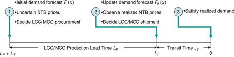
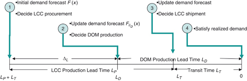
In the diversification strategy, the firm first decides its LCC and MCC procurement quantities, q 0 and q 1, and then later decides its LCC and MCC shipment quantities, y 0 and y 1, to DOM. We count the time backwards and adopt the convention that the selling season occurs at time 0. Recall that we assume LCC and MCC have the same lead time and, therefore, the firm makes its LCC/MCC procurement decisions simultaneously at time L P +L T . The same is true for the shipment decisions at time L T . We have a three‐stage stochastic decision problem and the sequence is as follows. In the first stage, at time L P +L T , procurement quantities q 0 and q 1 are set. In the second stage, at time L T , after NTB prices and demand information gain θ have been realized, the shipment quantities y 0 and y 1 are set. In the third stage, at time 0, the remaining demand uncertainty is resolved and the firm uses its available inventory to fill as much demand as it can (see Figure 1).
In what follows, we first characterize the firm's second‐stage shipment problem (the third stage is trivial), and then characterize its first‐stage procurement problem. In the second stage, the firm observes the realized NTB prices z
0 and z
1 and the information gain θ. The firm's problem is to determine the shipment quantities y
0 and y
1 from LCC and MCC. Let  . The second‐stage expected profit function is
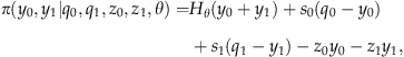
We are now in a position to characterize the firm's first‐stage problem. Let  denote the firm's first‐stage expected profit function conditional on the realized information θ. Substituting the optimal shipment decisions
  and
and  from Lemma A1 in the Appendix into (1), and taking the expectation over z
0 and z
1, we have
from Lemma A1 in the Appendix into (1), and taking the expectation over z
0 and z
1, we have 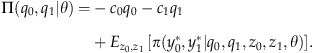
T is jointly concave in q
0
and q
1. (b) The firm's first‐stage expected profit function,
is jointly concave in q
0
and q
1. (b) The firm's first‐stage expected profit function, 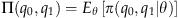 , is jointly concave in q
0
and q
1.
, is jointly concave in q
0
and q
1.
Because the expected profit function is well behaved, the firm's first‐stage production quantity can be uniquely determined. Closed form solutions, however, will not typically exist.
Having partially characterized the general diversification model, we now analyze the direct and split strategies. To allow further characterization, for the remainder of this subsection (section 4.2) we assume that the firm observes the realized market demand by shipment time, i.e., θ completely resolves demand uncertainty. This approximates the situation where the transportation time is short relative to the production lead time, a situation which can sometimes arise in the clothing industry. While the ratio of the production lead time to the transportation time for men's jeans sourced from coastal China is approximately 2:1 (Abernathy et al. 2005), the ratio for other textile products and other Asian countries can be 3:1 (Nuruzzaman 2009) and even as high as 9:1 (Volpe 2005).
4.2.1. Split Procurement
In the split procurement strategy, the firm procures from two countries, LCC and MCC, where LCC is subject to NTBs but MCC is not. This model can be obtained by setting z
1≡0, indicating there is no NTB risk associated with MCC. Substituting z
1≡0 into (1), we obtain the second‐stage profit as  . The optimal shipment quantity is obtained as a special case of Lemma A1 in the Appendix:
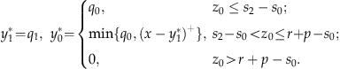
C and
and  either equal zero or jointly satisfy the following two equations.
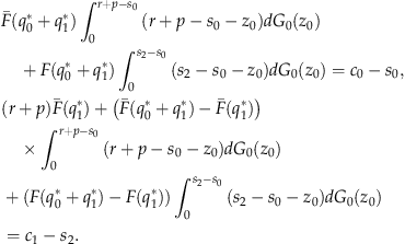
4.2.2. Direct Procurement
In the direct procurement strategy, the firm single sources from LCC which is subject to NTBs. This model can be obtained from the general diversification model by setting z
1≡∞ which makes MCC an infinite cost country. Substituting z
1≡∞ into (1), we have y
1≡∞ and the firm's second‐stage profit is  , where
  , reflecting the fact that θ completely resolves demand uncertainty. The optimal solution to the direct procurement's second‐stage (shipment) problem is obtained as a special case of Lemma A1 in the Appendix:
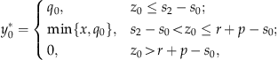
In this case, regardless of the size of the realized demand, the firm ships the finished product if and only if z
0≤r+p−s
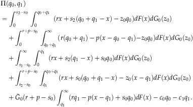
0, i.e., the realized NTB price is less than the unit profit foregone by not shipping. Substituting (5) and z
1≡∞ into (2) (and taking the expectation over X), we have 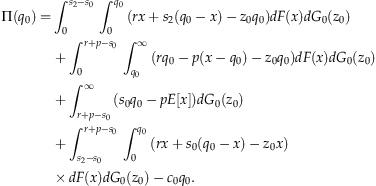
C
 .
.
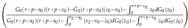
If the NTB price is equal to zero with probability 1, then 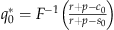 , which is the familiar newsvendor quantity. This needs to be appropriately adjusted (as specified in Corollary 2) to account for the stochastic NTB price and the fact that the decision to ship or not is made after demand is realized. The following corollary establishes some basic sensitivity results for both the direct procurement and split procurement strategies.
C
The above corollary characterizes the directional impact of basic system parameters on the firm's optimal expected profit. These sensitivity results are quite intuitive.
4.3. Outward Processing Arrangement
In the OPA strategy, the firm procures a fraction of the product domestically and procures the rest from an LCC. The OPA strategy completely removes NTB controls, but the firm must maintain a certain level of domestic production to qualify. That is, domestic (DOM) procurement must exceed a certain fraction of the total (DOM and LCC imported) procurement. The severity of the domestic procurement constraint, i.e., the minimum fraction, is a policy decision made by the competent authorities, e.g., the Department of Trade and Industry, in the firm's domestic country (see EEC Regulation No. 2913/92, e.g.). 7
Recall that we use q
2 to denote the firm's DOM procurement quantity and y
0 to denote the quantity imported from LCC. Let 0≤α≤1 denote the competent‐authority imposed fraction of total (DOM plus LCC) procurement that the firm's domestic procurement must satisfy. That is, the firm's domestic procurement quantity q
2 must satisfy 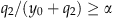 . The fraction α is a policy‐level decision that reflects the competent authorities' desire to maintain domestic employment opportunities and production capabilities. For the rest of this section, we let θ
D
denote information gained by L
D
, i.e., the time at which the DOM procurement is decided. Let
. The fraction α is a policy‐level decision that reflects the competent authorities' desire to maintain domestic employment opportunities and production capabilities. For the rest of this section, we let θ
D
denote information gained by L
D
, i.e., the time at which the DOM procurement is decided. Let  denote the updated demand distribution at time L
D
.
denote the updated demand distribution at time L
D
.
The firm faces a four‐stage stochastic decision problem and the sequence of events is as follows. In the first stage, at time L P +L T , LCC procurement decision q 0 is set. In the second stage, at time L D (recall that L T ≤L D ≤L P +L T ), DOM procurement q 2 is determined based on the updated demand distribution. In the third stage, at time L T , LCC import quantity y 0 is determined. 8 In the last stage, the firm fulfills as much demand as possible after demand uncertainty is resolved (See Figure 2). 9
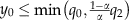
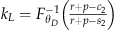
In what follows, we first consider the firm's third‐stage problem (the last stage is trivial). To satisfy the domestic procurement constraint, the firm's LCC import quantity y
0 must satisfy 0≤y
0≤(1/α−1)q
2. Because s
2≤s
0, we must have 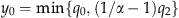 , regardless of the updated demand forecast at time L
T
. Since q
2 is determined at time L
D
, the firm can equivalently determine y
0 at time L
D
. The firm's second‐stage expected profit function is therefore
, regardless of the updated demand forecast at time L
T
. Since q
2 is determined at time L
D
, the firm can equivalently determine y
0 at time L
D
. The firm's second‐stage expected profit function is therefore 
 .
.
T
(a) The firm's second‐stage optimal expected profit function is concave in q 0.
(b) For any given LCC procurement quantity q
0
, the firm's second stage optimal shipment and DOM procurement decisions are given by the following: 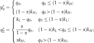
 and
and 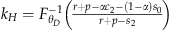 .
.
(c) The firm's second‐stage expected profit is given by 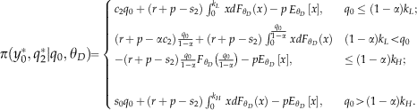
For a given LCC quantity q 0, the total inventory made available (imported plus domestically produced) is k L , q 0/(1−α) or k H depending on the updated demand distribution at time L D . In the latter two cases, the domestic fraction constraint α is binding but it is not in the k L case. Now, k L is the newsvendor produce‐up‐to level for DOM, indicating that the firm produces the optimal domestic quantity without having to adjust for the domestic constraint. In contrast, k H is the newsvendor produce‐up‐to level for a marginal cost of αc 2+(1−α)s 0. To understand this produce‐up‐to level, consider that an additional unit of inventory is created (subject to the binding domestic constraint) by producing α domestically and importing (rather than salvaging) 1−α from LCC; thus the effective marginal cost is αc 2+(1−α)s 0.
Given the characterization of the firm's second‐stage problem, the firm's first‐stage problem can be expressed as  .
.
T
Therefore, there exists a unique  that maximizes the firm's first‐stage expected profit. We note that this characterization is very general with respect to the forecast evolution process; the result holds as long as the information gained is non‐decreasing over time.
10
that maximizes the firm's first‐stage expected profit. We note that this characterization is very general with respect to the forecast evolution process; the result holds as long as the information gained is non‐decreasing over time.
10
5. Managerial and Policy Implications
We now explore how the firm's strategy preference (direct, split, or OPA) is influenced by certain industry and country characteristics. We ignore any fixed costs associated with a strategy, e.g., a fixed cost associated with locating in a particular country, as the directional effects of fixed costs are clear. We first describe the numerical study used to augment some of our later analytical findings. The study comprises 1,102,500 problem instances (described in Table 1). We kept the DOM cost at c
2=1 and so the other cost and revenue parameters are essentially scaled relative to the DOM cost. Because we adopt a CNF type of contract in which the LCC and MCC procurement costs, c
0 and c
1, include transportation, we explicitly call out the transportation cost in our numerical study and denote it as c
t
. This allows us to vary the percentage of cost associated with transportation and also to relax the assumption that s
2≥s
1. We use a Weibull distribution for the NTB price in our numerical study because it has a non‐negative support and can assume various shapes. We also assume a normal distribution for some of analytic results in this section. One key difference between the Weibull and the normal distribution is that the former is not symmetric whereas the latter is.
11
At the start of the planning horizon, i.e., at time L
P
+L
T
, the firm faces an identical demand distribution regardless of which strategy the firm uses. We adopt a linear martingale process for the demand forecast evolution, i.e., forecast revisions are independent, identical, and normally distributed. For each of the 1,102,500 problem instances we computed the optimal profit for each strategy using a grid search technique. When applicable the search took advantage of the concavity results established in this paper by using a bisection search. Let  ,
,  , and
, and  denote the optimal profit for the direct, split, and OPA strategies, respectively.
min∼max (step size).
5.1. Managerial Implications
In what follows, we explore the impact (direction and magnitude) of changes in the level and predictability of NTB prices, the LCC cost and transportation cost percentage, the domestic lead time and OPA production constraint, and the demand uncertainty and unit revenue.
5.1.1. Level and Predictability of NTB Prices
Some NTBs are highly uncertain due to their allocation structure, e.g., safeguard measures and voluntary export restraints, whereas other NTBs may be high but with little uncertainty, e.g., when an industry‐level antidumping duty has been determined and is expected to last for a number of years. We first consider stochastic rankings of NTB prices and then explore the impact of changes in the mean and variance of NTB prices.
A random variable Z
a
is (first‐order) stochastically dominated by another random variable Z
b
if, for any given value of z, G
a
(z)≥G
b
(z), where G
a
(·) and G
b
(·) are the distribution functions of Z
a
and Z
b
, respectively. We say that Z
b
is stochastically larger than Z
a
, and denote this by  .
.
T denote two possible NTB prices in LCC. All else equal,
  under Z
0
b
is less than that under Z
0
a
, and
under Z
0
b
is less than that under Z
0
a
, and  under Z
0
b
is less than that under Z
0
a
.
under Z
0
b
is less than that under Z
0
a
.
Therefore, a stochastically larger NTB price hurts the DIR and SPL strategies. 12 Interestingly, however, a higher NTB price variance can benefit the DIR and SPL strategies.
T and
and  decrease in μ and increase in σ.
The standard deviation (or, equivalently, variance) result can be explained as follows. The firm's downside exposure to a very high NTB price is bounded by the firm's postponement option of not shipping the finished product (in which case the firm avoids paying the high NTB price but incurs the penalty cost for unfilled demand). However, the upside advantage of a very low NTB price is significant. This asymmetry between the bounded downside disadvantage and the upside advantage benefits the firm as the NTB price variance increases.
Turning to our numerical study, Figure 3 illustrates the impact of the NTB price mean and coefficient of variation (CV) on the relative profit differences between the three strategies. For each mean/CV pair, Figure 3a shows the relative profit difference between the DIR and SPL strategies, where the number reported is the average of all problem instances with that mean/CV pair. 13 Figures 3b and 3c show the relative profit difference between OPA and DIR and between OPA and SPL, respectively. In Figures 3b and 3c, we see that both DIR and SPL become less attractive relative to OPA as the mean (CV) NTB price increases (decreases). Because the OPA strategy is unaffected by the NTB characteristics, this observation indicates that both the DIR and SPL profits decrease (increase) in the mean (CV) of the NTB price. A similar finding to Theorem 5 therefore holds even when the NTB price has a Weibull rather than a normal distribution.
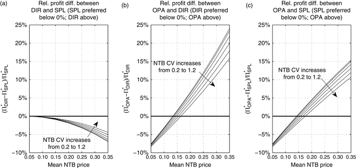
While the directional result is important, it is interesting to observe the magnitude of the effect of the NTB mean and CV. Consider the oil pipe example mentioned in section 1: some firms were hit with a (provisional) 36.53% countervailing duty while others were hit with a (provisional) 99.14% duty, or equivalently the expected levy was 2.7 times higher for some firms than for others. Looking at Figure 3b, we see that an increase in the mean NTB price from 0.1 to 0.27 (i.e., by a factor of 2.7) 14 drives the relative profit difference between OPA and DIR from approximately −3% to 13% for a CV of 0.2. In other words, OPA goes from being somewhat worse than DIR to being very significantly better. 15 So, differences in the mean NTB price that are reasonable (given observations from practice) can have a profound impact on strategy. The NTB price CV also has a material impact, with changes at higher CVs, e.g., from 1.0 to 1.2 being more significant than changes at lower CVs, e.g., from 0.2 to 0.4.
Finally we note that if the NTB price mean (CV) is low (high), the SPL strategy sources almost exclusively from LCC and so its profit is only slightly better than DIR (see Figure 3a).
5.1.2. LCC Cost and Transportation Cost
While an increase in the LCC procurement cost hurts all strategies, it is not immediately obvious how changes in the LCC cost will influence the relative ranking of the strategies. We address this through our numerical study. Figure 4 shows the impact of the LCC procurement cost c 0 and transportation cost c t on the relative profit differences.
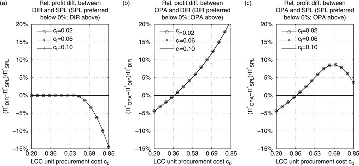
Focusing first on the LCC cost c 0, DIR becomes less attractive compared with SPL or OPA as c 0 increases. At low values of c 0, SPL is not concerned about the NTB price risk and sources exclusively from LCC, and so DIR and SPL have the same profit (see Figure 4a). As c 0 increases the NTB price risk becomes a larger concern as the NTB adds to the effective LCC cost; therefore, SPL sources a larger fraction from MCC to hedge against the NTB price. DIR cannot hedge and so SPL is increasingly favored over DIR as c 0 increases. Comparing DIR and OPA (Figure 4b), DIR becomes less attractive as c 0 increases because OPA has the option of sourcing more domestically and the domestic cost disadvantage decreases as c 0 increases. This finding can be proven under certain technical conditions (details available upon request). Observe that the relative profit difference is very sensitive to the LCC cost, indicating that small changes to the LCC cost may significantly impact strategy preference even when fixed costs are considered. 16
Comparing SPL and OPA (Figure 4c), the relative profit difference is not monotonic in c 0, indicating that an increase in the LCC cost may benefit or hurt OPA (relative to SPL) depending on the current LCC cost. When c 0 is low, an increase hurts SPL because SPL sources a large fraction from LCC but OPA's LCC production is constrained by the domestic production constraint. When c 0 is very high (i.e., close to the MCC cost), an increase hurts OPA because SPL sources almost exclusively from MCC while OPA still sources some portion from LCC.
Turning now to the transportation cost c t , we see from Figure 4 that it has a negligible impact on the relative profit differences. Recall that the LCC and MCC costs, i.e., c 0 and c 1 include the transportation cost as we adopt the CNF‐type contract, and so varying c t for a fixed c 0 and c 1 does not change the total procurement cost but does change the portion spent on transportation. Because the strategies can choose not to ship product after demand is realized, the transportation cost does influence profit somewhat but it does not have a large impact on the relative profits (for the values chosen in the numeric study).
5.1.3. Domestic Lead Time and OPA Production Constraint
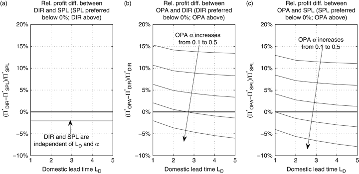
The OPA strategy engages in some domestic production, and we next explore the impact of the domestic lead time L D and the competent‐authority imposed domestic production constraint α. Because a shorter domestic lead time and less severe domestic constraint allows OPA to more precisely fine tune inventory based on updated demand information, the following theorem formalizes what one might expect, i.e., OPA benefits from shorter domestic lead times and lower domestic production constraints.
T decreases in the domestic lead time L
D
and production constraint α.
decreases in the domestic lead time L
D
and production constraint α.
Because both DIR and SPL are unaffected by L D and α, OPA becomes relatively more attractive as L D and α decrease (see Figure 5) 17 . Observe that both the lead‐time and the production constraint have a significant impact. While not shown in the figure, the effect of the domestic lead time is much more pronounced at higher initial demand CVs than at lower initial demand CVs. 18 This derives from the fact that the value of delaying domestic production (until a better demand forecast is obtained) is higher when initial demand uncertainty is higher.
5.1.4. Demand Uncertainty and Unit Revenue
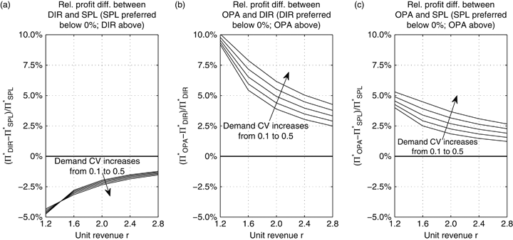
We now consider market and product characteristics, focusing in particular on the demand uncertainty and product revenue. Figure 6 presents the relative profit differences as a function of the demand CV and the revenue r. The demand CV has a reasonably significant impact on the relative attractiveness of OPA compared with DIR and SPL, with OPA being increasingly preferred as the CV increases (see Figures 6b and 6c). It is not always true, however, that a higher demand uncertainty favors OPA; increasing demand CV can favor SPL and DIR if the DOM lead time is high and the mean NTB price is low (see the supporting information Appendix S3). The demand CV has only a small impact on the relative profit difference between DIR and SPL, whereas the unit revenue r has a moderate impact (see Figure 6a). The relative profit difference between OPA and either DIR or SPL decreases in r, quite significantly in the case of DIR. However, one needs to interpret the directional effects of r in Figure 6 with some caution. While the relative profit difference between OPA and either DIR or SPL decreases in r, the actual profit difference increases. Likewise the actual profit difference between DIR and SPL decreases although the relative profit difference increases. (For all other parameters explored in this study, the relative and actual profit differences exhibited the same behavior.) As strategy choice will be determined by the actual profit difference, OPA is favored as the revenue r increases because the domestic cost disadvantage is less pronounced if the unit revenue is high.
5.2. Policy Implications
The firm must maintain a certain level of domestic production to qualify for an OPA strategy. The minimum DOM procurement fraction α is a policy decision made by the competent authorities in the firm's domestic country (see EEC Regulation No. 2913/92, e.g.). The mandated minimum fraction, which can vary from one product category to another, reflects a desire to promote domestic employment but is often influenced by the lobbying efforts of firms. From a policy perspective, it is of interest to understand whether (i) a higher value of the mandated fraction does lead to a higher domestic production level, and (ii) how much emphasis authorities should place on industry characteristics (beyond firms' lobbying capabilities) in setting the mandated fraction.
As to question (i), our numerical study found that, if the firm is committed to the OPA strategy, a higher domestic constraint α does result in a higher expected domestic procurement quantity, although the total LCC plus DOM procurement quantity decreases. However, if the firm is not committed to the OPA strategy, then an increase in α may induce the firm to switch to a different strategy, thereby eliminating domestic production entirely. Such a switch defeats the competent‐authority's intent of setting α to promote domestic production. We define the switching fraction  as the value of α at which the firm switches from the OPA to the SPL strategy (recall that SPL weakly dominates DIR). Using the numerical study described in Table 1, we calculated the switching fraction
  for each instance by searching for the α value that resulted in the OPA profit being equal to the SPL profit. Figure 7 shows that
  is quite sensitive to both NTB price uncertainty (Figure 7a) and demand volatility (Figure 7b and c) unless the domestic lead time is long or the unit revenue is low. This suggests that, when setting the mandated OPA domestic procurement fraction, the competent authorities should pay attention to industry characteristics (demand and profitability) and NTB characteristics (mean and CV), and not just lobbying efforts, or they run the risk of unwittingly driving firms to abandon domestic production altogether, defeating the very intent of the OPA program. In particular, the competent authorities should mandate a lower α for industries with a stable market, or longer domestic procurement time, or lower average NTB price. In contrast, a higher α can be imposed for industries with a volatile market and a shorter domestic lead‐time advantage over the LCC.

6. Conclusion
In this paper, we explore three supply chain strategies used in industries subject to NTBs, namely, direct procurement, split procurement, and OPAs. We characterize the optimal procurement decisions in these strategies and provide managerial and policy insights. Among other findings, we establish that direct and split strategies benefit from NTB volatility (as measured by the variance of the NTB price) but suffer from increased NTB mean prices. Both the cost disadvantage and lead‐time advantage of domestic production are also significant influencers of the preferred strategy, as is the domestic‐country mandated production constraint associated with the OPA strategy. Policy makers seeking to maintain domestic production should account for these drivers when setting the mandated domestic production fraction for OPA qualification.
There are two situations in which our model of a single selling season coupled with a single‐order opportunity for LCC and MCC would not be appropriate. The first situation is where the LCC and MCC lead times are short enough to allow multiple orders even with one annual selling season. In our setting, OPA is the only strategy that can fine tune inventory with a second order. This advantage would be dampened if the LCC and MCC lead times allowed multiple orders. Analyzing this situation would require, among other things, careful thought about how to model the NTB price evolution. It is an open and interesting question as to if and how our findings would change in such a setting. The second situation that our model does not capture is that of a functional product (Fisher 1997), i.e., a product with a long life cycle. Certain functional products are prone to trade disputes, e.g., tires and oil pipes in our introduction, and it would be of interest to explore NTB risk for functional products. An infinite‐horizon model would be more applicable to such a setting. Again, the modeling of the NTB price would require careful thought. Stochastic price models, e.g., Kalymon (1971), might offer some pointers. Both of these settings merit exploration.
In closing, we discuss other directions for future research. The supply chain strategies studied span countries and because the firm's purchasing contract may not always be written in its domestic currency, it might be fruitful to explore how exchange rate risk influences strategy preferences. It would also be interesting to explore the strategic interactions between the supplier and the buyer. For example, in the direct procurement and the split procurement strategies, a firm can sometimes negotiate with its supplier to jointly share the NTB risk. While many of our findings on firm preferences are supported by anecdotal evidence from the textile industry, there might be opportunities for empirical research to shed further light on what influences a firm's strategy choice.
Footnotes
Appendices
Acknowledgments
The authors would like to thank the associate editor and the two referees for their comments and suggestions, which significantly improved this paper.