A Note on the Relationship Among Capacity,Pricing,and Inventory in a Make‐to‐Stock System

Abstract

We address the simultaneous determination of pricing, production, and capacity investment decisions by a monopolistic firm in a multi‐period setting under demand uncertainty. We analyze the optimal decision with particular emphasis on the relationship between price and capacity. We consider models that allow for either bi‐directional price changes or models with markdowns only, and in the latter case we prove that capacity and price are strategic substitutes.

Keywords

capacity investment pricing inventory stochastic demand

1. Introduction

1.1. Background and Overview of Main Findings

Recent years have witnessed an increased interest in the use of pricing in operations management practices, with a particular focus on the integration of inventory control and dynamic (state‐dependent) pricing strategies. Concomitantly, studies focusing on the interface between capacity investment and replenishment strategies have led to further understanding of capacitated inventory systems and supply chains. A very useful qualitative insight in this context has been the understanding that capacity and inventory are in essence strategic substitutes. Roughly speaking, decision variables are said to be strategic substitutes if increasing the value of one variable decreases the return from increasing the other; a more precise definition will be advanced in section 4. One of the main motivations for the present paper is to develop similar insights that pertain to pricing and capacity decisions. As the literature review at the end of this section indicates, we are only aware of a few papers to date that focus on the problem of joint capacity planning and pricing strategies, and even less that go on to explore the three‐way relationship between capacity, inventory, and pricing decisions.

In this paper, we study a stylized problem in which a centralized monopolistic firm sells a product over a finite selling horizon; the number of periods constituting this time horizon measure the time elapsed from the first introduction of the product to the market, up until the point where the firm terminates its production and sale. The firm reviews the state of the system periodically and at the beginning of each period makes three decisions: (i) invest or disinvest in production capacity, (ii) replenish inventory (constrained by production capacity), and (iii) fix a price for the produced goods that will take effect in the following period. Subsequent to these decisions, demand is observed. We first allow the firm to carry inventory from one period to the next, and orders are allowed to be backlogged. Subsequently, we introduce a restriction that disallows carry‐over of inventory from period to period; the firm must then either satisfy inventory shortage using emergency replenishment or by paying penalty fees. In the next stage, we also restrict the firm's pricing flexibility by only allowing markdowns, i.e., the price of the product can only decrease over its life cycle.

The main contribution of this paper is in studying the relationship between pricing and capacity decisions in the context of a dynamic optimization problem that has capacity, inventory, and price as its variables. The analysis proceeds by first showing that the optimal capacity investment policy in the presence of pricing and inventory decisions is of a target interval form (see Theorem 1). Given a fixed capacity level, the optimal joint pricing–inventory decisions are seen to follow a modified base‐stock list‐price policy (see Theorem 2). These results serve as a basis for studying a model where no inventory carry‐over is allowed, and pricing is restricted to markdowns. In this important scenario we show that price and capacity are strategic substitutes both as decision variables and as state variables (see Theorem 3); an important implication is that these levers can be used in a complementary manner (see discussion in section 5.3). Several numerical examples illustrate some of these findings.

This section concludes with a review of related literature and known results. Section 2 describes the model and sets up the dynamic optimization problem. Section 3 provides the first set of results. Section 4 discusses the cases where no carry‐overs are allowed and when pricing is restricted to markdowns. Section 5 summarizes some qualitative insights that are gleaned from the main results and also provides a simple example that illustrates the key findings. All proofs are collected in the supporting information Appendix S1.

1.2. Literature Review and Positioning of the Present Paper

Given the voluminous literature on the topic of interest in this paper, we restrict our review to work that is closely related in terms of thrust and problem formulation. For a recent survey and further references on pricing, inventory, and capacity decisions the reader is referred to Chan et al. (2004, section 4.2).

1.2.1. Inventory Decisions in Capacitated Systems. Federgruen and Zipkin (1986) consider a single‐item, periodic‐review inventory model with uncertain demands. Under the assumption of finite production capacity in each period, they show that a modified basic‐stock policy is optimal. Some extensions include Aviv and Federgruen (1997) that deals with non‐stationary demand, and Ozer and Wei (2004) that deals with information acquisition and replenishment costs.

1.2.2. Inventory and Pricing Decisions. Federgruen and Heching (1999) study the relationship between price and inventory in an uncapacitated system with stochastic demand. They characterize the structure of the optimal price–inventory policy, and show that inventory and price are strategic substitutes. Further references in this stream of literature are surveyed in Elmaghraby and Keskinocak (2003); a deterministic analysis of such problems dates back to Thomas (1974) and Kunreuther and Schrage (1973). Recently, Ketzenberg and Zuidwijk (2009) studied the joint pricing, ordering decisions, and return policies for consumer goods, and Huh et al. (2010) studied the optimal pricing and production for subscription‐based products.

1.2.3. Inventory and Capacity Decisions. Angelus and Porteus (2002) study capacity decisions in cases where a firm can and cannot hold inventories. In the former case, they establish that capacity and inventory are strategic substitutes. (For an example of an analysis of a deterministic model, see Rao 1976.) Eberly and Van Mieghem (1997) study a problem that can be viewed as a generalization of the “no‐carry‐over” version of Angelus and Porteus (2002). They characterize the optimal capacity policy when capacity is multi‐dimensional and it is costly to reverse capacity investments. Duenyas and Ye (2007) generalize Angelus and Porteus' (2002)“no‐carry‐over” model by allowing fixed and variable costs in capacity adjustments.

1.2.4. Joint Pricing, Production, and Capacity Decisions. Maccini (1984) studies the effects of inventory dynamics and capital on pricing and capacity decisions from a macroeconomic perspective. He finds that excess capacity tends to cause prices to decrease below their acceptable long‐run levels. Gaimon (1988) shows, by means of a numerical study, that upgrading capacity lowers the firm's per unit production cost and thus the prices it charges. Li (1988) introduces a point process model of a production firm with intensities parameterized by production, capacity, and price, respectively. A distinction is made between static decision making (capacity levels are set at time zero), and dynamic operating decisions (pricing and production). Van Mieghem and Dada (1999) study different possible postponement strategies in a single‐period problem when firms make three decisions: capacity investment, production (inventory) quantity, and price. (See also Boyaci and Ozer 2007 for a study of information acquisition through advance selling.)

A notable entry absent from the above list is work focusing on joint pricing and capacity decisions in an inventory setting, and the present paper indeed strives to fill that gap. In terms of the model and analysis tools, our work is most closely related to that by Angelus and Porteus (2002) and Federgruen and Heching (1999): the former studies the relationship between inventory and capacity, and the latter discusses inventory and prices. Our research is intended to complement theirs.

2. Problem Formulation

We consider a monopolistic firm that produces a single product whose capacity, inventory, and price are reviewed periodically. At the beginning of each period the firm makes three decisions: (i) capacity investment (or disinvestment), (ii) production level, and (iii) the price it will charge for the product. We assume that capacity investments and produced goods become available instantaneously. The life cycle of the product, and therefore the time horizon, is set to be T periods. The sequence of events in each period, t=1, …, T, is as follows:

Investment or disinvestment in capacity, setting it to a level equal to z _t.

Production (if needed) to set the inventory level to y _t.

A price p _t is set and held fixed up until period t+1.

Demand is realized and satisfied if it is less than available inventory, or backlogged otherwise. Backlog and holding costs are incurred.

Demand in period t, D _t, depends on the prevailing price which is given by a general additive stochastic demand function 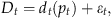1 where p _t is the price charged in period t and ɛ _t is the sequence of independent random variables.

Feasible price levels are confined to the interval , where and are the highest and lowest prices, respectively. (In sections 4 and 5, we indicate how the main results extend to more general demand functions.)

Let x _t be the inventory level at the beginning of period t before ordering and y _t be the inventory level at the beginning of period t after ordering. The firm incurs two types of production and inventory costs: the end‐of‐period inventory carrying (and backlogging) costs, and a variable production cost. Specifically, h _t(x) is the inventory (or backlogging) cost incurred in period t with terminal inventory level equals x and c _t is the per unit purchasing or production cost in period t.

Let 2 denote the single‐period expected inventory and backlogging costs for period t, for a given price p and an inventory level (after ordering) y, where the expectation here, as well as in the remainder of the paper, is taken with respect to the distribution of the random noise term. We assume that:

(A1)

, for all t=1, …, T,

(A2)

h _t(·) is convex for all t=1, …, T.

(A3)

d _t (p _t, ɛ _t)=a _t−b _t p _t+ɛ _t where a _t, b _t>0, , for all t=1, …, T.

These assumptions ensure that the cost functions G _t(y, p) are well defined, finite, and jointly convex in y and p for all t=1, …, T.

 Remark 1. The assumption of linear demand can be generalized to any demand function which is continuous and strictly decreasing in the price variable, and for which the revenue rate is concave in d, where d _t ⁻¹ is the inverse function of d _t for fixed ɛ _t. This assumption is rather benign and quite standard in the revenue management literature; Ferguson et al. (2006) provide examples of a linear function and an exponential demand function that satisfy these conditions; see also Chen and Simchi‐Levi (2002) for further discussion. In that case, one would need to impose directly that G(·,·) is jointly convex; see Federgruen and Heching (1999) for conditions ensuring that this holds.

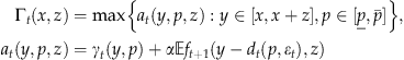
Let γ _t (y, p) denote the expected contribution in profits in period t, if the firm has y units at the beginning of the period (i.e., post‐production) and it charges p per produced unit that is sold on the market. That is, in period t 3 Let z _t be the capacity level at the beginning of period t after adjustment. We define three capacity related costs: K, the cost of adding a unit of capacity; k, the return from selling a unit of capacity; h _c, the capacity overhead cost per unit.

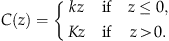
Hence h _c amalgamates all costs that are associated with maintaining production, but are independent of the production volume. We assume that K≥k, which reflects the fact that capacity is usually sold for less than the purchase price. Revenues and costs are discounted with a discount factor α∈(0, 1]. We note that all capacity‐related costs are taken to be time‐homogeneous for simplicity, and the analysis that follows can easily be adjusted to account for such temporal dependency. We assume that a firm begins the life cycle of the product with capacity level z ₀ and inventory level x ₀ (allowing for the possibility of x ₀=0, z ₀=0). Note that our work pertains primarily to industries in which there is short lead time for capacity changes, as well as low fixed costs for capacity changes (apart from the friction of selling–buying). In industries, such as medical devices, in which soft‐tooling is being used, such quick capacity changes are possible.

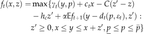
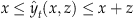
Let f _t(z, x) be the maximum expected present value of the total net profits that can be earned in months t and on, given that the capacity level is z and inventory level is x at the beginning of period t. That is, 4 for t=1, …, T, where 5 At the terminal period, we assume that demand is satisfied and the remaining capacity is sold immediately thereafter, that is, we set

To recapitulate, at the beginning of each period t=1, …, T, the firm must determine a capacity investment level z′, an inventory level y, and a price p based on the initial inventory and capacity, x and z. These decisions are held fixed throughout period t. The objective of the firm is to maximize the sum of discounted profits over the time horizon T with respect to the above‐mentioned decision variables; the maximum value of this dynamic optimization problem is given by f ₁(x, z).

For future purposes it will be convenient to rewrite f _t(x, z) as follows (see Angelus and Porteus 2002): 6 where 7 for all t=1, …, T.

3. The Optimal Policy and Key Relations

3.1. Main Results

In this section, we characterize the structure of a policy that maximizes the expected discounted profits. The results are very much in the spirit of those in Federgruen and Heching (1999) (albeit for a non‐capacitated system) and Angelus and Porteus (2002) (for a model with exogenously given prices).

Recall, the maximum value of this objective is given by f ₁(·,·), where f _t(·,·) is defined in (6). We will begin by analyzing the optimal capacity investment policy. Then, given the optimal capacity at the beginning of a period, we will derive the optimal joint inventory–pricing policy. It is important to note that the three decisions are made simultaneously; the optimal policy is described in a sequential manner to allow for a more transparent representation.

To characterize the optimal capacity investment policy, we first describe a family of ISD policies (invest/stay put/disinvest), often referred to as target interval policies.

 Definition 1. A sequence {z _t}_t=1 ^T constitutes a target interval policy with respect to a sequence of non‐negative real numbers {L _t, U _t}_t=1 ^T, if

(i)

L _t≤U _t;

(ii)

L _t and U _t are independent of z _t−1;

(iii)

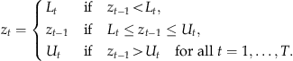
The upper and lower targets L _t and U _t can be functions of the state of the system (and past information observed up until time t), and the notation L _t(·) and U _t(·) will be used to indicate this dependence; in the following theorem, both are functions of the initial inventory x.

Theorem 1. (Optimal capacity investment policy) The optimal capacity investment decision follows a target interval policy in each period, with lower‐ and upper‐capacity targets L _t(x) and U _t(x) for each t=1, …, T and each initial inventory level . 

Based on the optimal capacity investment, we will now show that the optimal joint production–pricing decision takes the form of a modified base‐stock list‐price policy (we use the term “modified” because of the capacity constraint on the production). 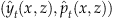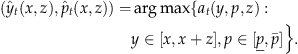This policy is characterized by a base‐stock level and a list‐price combination which are given as a function of the initial inventory and capacity (x, z); the former and latter functions are the optimal inventory position and price levels, respectively, given that period t begins with capacity z and inventory level x, and are derived as follows: The existence and uniqueness of and for given initial capacity and inventory levels, x and z, are established in the proof of Theorem 2. Note that the “hat” notation is used to distinguish the optimal policy. For the purpose of the following theorem, we introduce the following definitions.

 Definition 2. Variables are said to be strategic substitutes with respect to a function 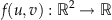, if f(u, v) is submodular in u and v. 

For a definition of submodularity, see, e.g., Topkis (1978), and for further discussion of economic implications and interpretation, see, e.g., Milgrom and Roberts (1990).

 Theorem 2. (Optimal pricing–inventory policy)

(a)

An optimal inventory–pricing policy is a base‐stock list price with base‐stock and list price for t=1, …, T. At period t∈{1, …, T}and given a capacity level z: if , it is optimal to order up to the base‐stock level and to charge the list price ; if , it is optimal not to order and to charge ; and if , it is optimal to order z units and charge .

(b)

For each period t∈{1, …, T}and fixed capacity and inventory state values , the price and inventory decision variables (y _t, p _t) are strategic substitutes with respect to the function a _t(·,·,z) given in (7) .

 Remark 2. (Discussion) The result of the theorem states that if the inventory level, x, is below the base‐stock level, it is increased to that value and the list price is charged. If the inventory level is above the base‐stock level, then nothing is ordered, and a price discount is offered, i.e., the price charged is below the list price. (The higher the excess in the initial inventory level, the larger the optimal discount offered.) If the sum of inventory and capacity is below the base‐stock level, the maximum possible amount is produced (i.e., the production level equals the capacity level), and the price charged is higher than the list price. No discounts are offered unless the product is overstocked, and no higher than list prices are charged unless the product is in shortage, which happens when the current capacity is not sufficient to support the “desired” inventory level. Numerical illustrations of this result are given in section 5.

 Remark 3. (Structural results) The proof of the theorem establishes certain monotonicity results for y _t(x, z) and p _t(x, z) with respect to the variables x and z. For example, Lemma 3 establishes that y _t(·, z) is non‐decreasing. The results of Lemma 4 imply that p _t(·, z) is non‐increasing. Similar statements can be derived for the dependence on z for the post‐adjustment capacity.

4. Joint Capacity Planning and Pricing

In this section, we analyze a particular instance of the joint capacity planning and pricing problem when inventory cannot be carried over from period to period and prices can only be decreased throughout the time horizon. This situation arises when firms cannot use inventory produced in “off‐peak” periods to absorb “peak‐demand.” To this end, we assume that stockouts are satisfied at the end of the period in which they occur; Federgruen and Heching (1999) describe such a mechanism as emergency purchases or production runs.

4.1. Main Results

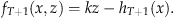
Let f _t ^M(z, p) denote the maximum expected present value of the total profits that can be earned in periods t up until T, given that period t starts with capacity z and price p. The optimality equations for t=1, …, T are given by 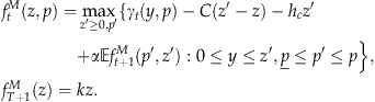The decision variables in the above equation are the price (p′) and capacity (z′) set in period t. We then have the following result.

 Theorem 3. Assume a firm cannot carry inventories and increase prices from period to period. Then, the following properties hold for all t=1, …, T:

(a)

f _t ^M(z, p) is submodular and jointly concave in the state variables (p, z).

(b)

The decision variables p′ and z′ are strategic substitutes with respect to f _t ^M(·,·).

(c)

The optimal capacity policy is a target interval policy in each period. The capacity targets L _t(p) and U _t(p) satisfy L _t(p)≤U _t(p) for each t=1, …, T, and each initial price p.

(d)

L _t(p) and U _t(p) are non‐increasing in p for each t=1, …, T.

Note that the upper and lower barriers L _t(·), U _t(·), t=1, …, T, are now functions of the price in the beginning of the period, unlike the case where inventory carry‐overs and bi‐directional price changes are allowed, in which case these barriers were functions of the inventory level in the beginning of the period.

 Remark 4. The model can be extended to treat non‐linear demand functions by assuming that is concave in p and that G _t(y, p) is jointly concave in (y, p) for all t=1, …, T. The first condition is easily satisfied for a broad family of demand functions. For a discussion of conditions that ensure the joint concavity of G _t(·,·), see Federgruen and Heching (1999).

5. Discussion and Qualitative Insights

5.1. An Illustrative Example of the Joint Pricing–Inventory–Capacity Model

5.1.1. A Two‐Period Problem with Quadratic Holding Costs. To illustrate the relationship highlighted in Theorem 2, we analyze a two‐period problem (one period in which a decision is being made and a terminal period). The demand in period t=1, 2 is given by d _t(p _t,ɛ _t)=a _t−b _t p _t+ɛ _t and the inventory holding cost is given by h _t(x)=hx ². Thus we obtain that G _t(y, p)=h[σ _t ²+(y−a _t+b _t p _t)²] and γ _t(y, p)=p(a _t−b _t p)−c _t y−hσ_t ²−h(y−a _t+b _t p)², where σ _t ²=Var(ɛ _t). Note that f _T+1(x, z)=kz−hx ². It is easy to show that 8 Put φ≡b _T+((α+1)h)⁻¹. Then the optimal pricing–inventory policy (given capacity z) can be described as follows:

•

if , order up to and set price to ;

•

if , order z units and set price to ;

•

if , order no more units and set price to .

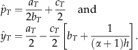
One can observe that, given the capacity level (after adjustment), z, the target inventory level at the beginning of the period is independent of the inventory level at the end of the previous period, x if x<a _T/2−c _T φ/2<x+z. Otherwise, keeping the capacity level fixed, the target inventory level is increasing linearly in x. Note that changing x may affect the optimal capacity level, and thus, indirectly affect the optimal inventory level. We next study the impact of the optimal capacity on the optimal ordering policy. It is easy to see that, unless a _T/2−c _T φ/2>x+z, the optimal target inventory level is independent of z.

In order to find the optimal capacity policy we need to compute the boundary functions L _T(x) and U _T(x). It is straightforward to show that where M is a constant that depends explicitly on the problem parameters.

Thus, the width of the inactivity band can be computed in closed form and we observe that, as anticipated, the inactivity region increases with the difference between the cost of increasing capacity, and the price for sold capacity. Moreover, we observe that as the initial inventory level increases, both the upper level and the lower level of the inactivity region decrease, and thus as the inventory level increases, the optimal capacity level (weakly) decreases.

Note that if the initial capacity level z ₀∈(L _t(x), U _t(x)), the capacity level is independent of the initial inventory. If this is indeed the case, the optimal inventory level depends on x only directly, as was discussed above. Thus, an increase in the initial inventory increases the target inventory level unless x<a _T/2−c _T φ/2<x+z ₀. Note that in this region, the target inventory level does depend on the initial capacity level, and it increases with the initial capacity level. In all other regions, the target inventory level does not depend on the initial capacity level, but may depend on the target capacity level.

If, on the other hand, z ₀>U _t(x), then . Note that, then, an increase in x, will decrease z, yet the sum of the two will remain constant. As the target inventory level depends only on the x+z, the target inventory level is independent of x, once x is above a level such that z ₀>U _t(x).

We observe that for fixed b _T, as the holding cost h decreases to zero, the inactivity region shrinks. Thus, capacity adjustments are always made if holding costs are negligible. At the same time, for any given value of h, if the price sensitivity b _T decreases to zero the inactivity region will remain proportional to the holding cost. Thus, the higher the holding cost, the less likely that capacity adjustments will be made. To summarize: as the holding cost increases or price sensitivity decreases, the value of adjusting capacity decreases. As mentioned above, the inactivity region also depends on the difference between the cost of purchasing capacity and its selling value. In many firms, capacity changes are fairly costly. In these cases the difference between the costs will increase the size of the inactivity region, thus allowing the firms to only modify price and inventory levels, while keeping the capacity level unchanged.

5.1.2. Numerical Illustration. Consider a firm that produces and sells a product during three periods, and a fourth period being the terminal one in which the firm sells off its capacity. The firm starts off with no capacity and zero inventory. Demand is anticipated to be low in the first period, increase during the middle period, and then return to its initial level in the final period. To encode this using our model parameters, we put a ₁=a ₃=5 and a ₂=10 in the demand function. We set b ₁=b ₃=1 and b ₂=2. For purposes of this example, we take the error term ɛ _t to follow a Poisson distribution with mean 1, independent for each period t=1, 2, 3. The firm's variable cost of production is c ₁=c ₂=c ₃=1. We set the holding cost to h(x)=h ⁺ max(x, 0)−h ⁻ min(x, 0), where h _t ⁻=1.9, and h _t ⁺=1.5 for t=1, 2, 3. The discount factor is α=0.9.

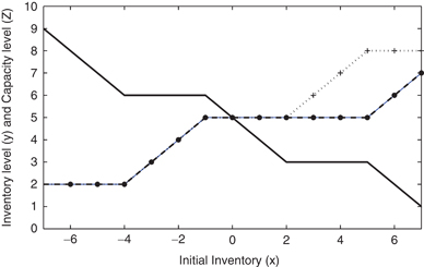
Figure 1 depicts the target inventory levels and optimal capacity levels for different levels of initial inventory. First, one can observe that in this case the optimal inventory level is a non‐decreasing function of the initial inventory level, and that capacity level is a non‐increasing function of the initial inventory. Note that the crossed line depicts the sum of the initial inventory and the optimal capacity level. This allows us to identify three production regions. As long as the initial inventory x is below 2, there is limited capacity and the firm sets the target inventory to x+z. When the inventory is the interval 2≤x≤5, the optimal inventory level is set to , which is independent of x and z. When the initial inventory level is >5, the target inventory is identical to the initial inventory, i.e., . The capacity policy is as follows: as long as the initial inventory is below 6, the capacity is set to the upper limit, which decreases with the initial inventory. Once the initial inventory reaches −4, the capacity level reaches the inactivity region, and the capacity remains unchanged until the inventory level reaches −1. Note that due to the change in the production region, the slope of the capacity function changes again around inventory levels 2 and 5. One can also observe that when z is below the lower limit (e.g., when −7≤x≤−4), x+z is kept constant, and thus the optimal inventory is independent of either, as predicted by the analysis of the two‐period model.

Figure 1

Optimal Capacity and Inventory Levels as a Function of Initial Inventory

5.2. Illustrative Examples of the Joint Capacity–Pricing Problem

5.2.1. Two‐Period Problem with Quadratic Holding Cost. We, again, analyze the two‐period model with quadratic cost in order to gain insights into the structure of the solution of the joint capacity–pricing model with no carry‐overs. One can show that, if p<a _T/2b _T+c _T/2, then  where A _T=a _T/2−c _T/2(1/h+b _T). We observe that once the current price is below this threshold level, it will remain at its current level. Note that if z>A _T, the firm's optimal capacity level is A _T, while if it is below we have to examine the upper and lower boundary functions. We observe that L _T(p)=a _T−b _T p−(c _T−αk+K−hc)/2h and U _T(p)=a _T−b _T p−(c _T−αk+k−hc)/2h. The inactivity region is given by ((K−k)(1−α))/2h. Note that here (i.e., when p<a _T/2b _T+c _T/2) the capacity inactivity region is independent of price. As the firm cannot use a price lever anymore, the decision whether to use the other two decision variables depends only on the ratio between the capacity cost difference (K−k) and the holding cost (h). If this ratio is “high” (i.e., cost of adjusting capacity is high relative to the holding cost), we expect the firm to restrict use to inventory in order to meet variability in demand.

In the region in which the initial price p>a _T/2b _T+c _T/2, we have that if z is below a certain level, and K≫k, then both price and capacity are kept fixed. As capacity is below the level A _T, the firm cannot further reduce price without incurring excessive shortage costs, and thus it will keep the price fixed. Capacity cannot change because related costs are too high. In this situation, inventory is essentially the only useful lever.

5.2.2. A Three‐Period Example Illustrating the Relationship Between Price Markdown and Capacity Investment Decisions. We again consider a firm that produces and sells a product during three periods; the fourth being the terminal period in which the firm sells off its capacity. The firm starts off with no capacity and zero inventory. Demand is anticipated to be low in the first period, increase during the middle period, and then return to its initial level in the final period. To encode this using our model parameters, we put a ₁=a ₃=8 and a ₂=10 in the demand function. We set b _t≡1 for t=1, 2, 3. For purposes of this example, we take the error term ɛ _t to follow a Poisson distribution with mean 1, independent for each period t=1, 2, 3. The firm's variable cost of production is c ₁=c ₂=c ₃=1. To reflect the fact that the firm cannot carry inventory and is thus inclined to resolve any excess demand within the period, we set h _t ⁻=3, h _t ⁺=1.5 for t=1, 2, 3. The discount factor is α=0.9.

Figure 2 is concerned with three capacity investment irreversibility values: K/k=2, 6, 8 (dotted, dashed, and solid lines, respectively). For each of these ratios, we computed the optimal policy that maximizes the average profit over the finite horizon using standard dynamic programming. The figure depicts the optimal policy under a “typical” path that is obtained by setting the noise variable ɛ _t to its mean value. We observe that as long as the ratio is lower than 6, the firm essentially uses the same pricing scheme, charging US$5, US$4, and US$3, and lowers the level of acquired capacity. However, once the ratio increases above 8, the firm utilizes a different pricing scheme, charging US$6, US$5, and US$4 while lowering the capacity level it purchases. As the firm can foresee that it will not be able to absorb demand using a high level of production (and capacity), and because it cannot increase its price in the middle of the product life cycle, it elects to charge a relatively high price in the first period even though the demand in this period is not greater than other periods.

Figure 2

Optimal Capacity and Price Levels for Different Capacity Investment Irreversibility Ratios K/k

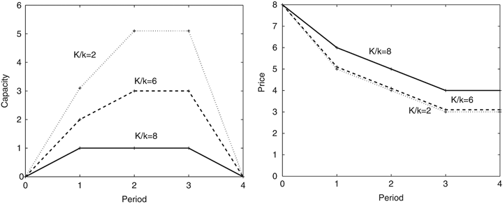
The firm then decreases prices in each subsequent period. In terms of capacity planning: the firm always invests in capacity in the first period, may invest in the second period (to accommodate the peak‐demand anticipated in period 2), and “stays put” in the third period (even tough demand is expected to be lower than in the second period). The above may be viewed as an illustration of complementarity between price and capacity. To wit, the first period commences with a relatively high price, and a relatively low level of capacity, leading to a high utilization of this capacity. In the second period, the firm increases capacity level to its maximum, and lowers price to increase demand. In the third period, because the firm already has acquired a significant level of capacity, it will again lower its price to allow for full utilization of the capacity, even though the expected demand is lower than that in the middle period.

5.3. Additional Discussion

5.3.1. Price and Capacity as Strategic Substitutes. The fact that price and capacity are strategic substitutes is equivalent to a complementarity relation between the level of capacity investment and the level of price decrease (relative to the maximum price ). The notion of complementarity that we are referring to is due to Edgeworth, according to which activities are considered complements if increasing the level of any one of them results in an increase in the return of engaging more in the other; see Milgrom and Roberts (1990, 1995) that summarize the principal results of the theory of supermodular optimization which underlies the notion of complementarity. They describe supermodularity as a way to formalize the intuitive idea of synergistic effects. In our example, a firm that coordinates sales planning and capacity investment has the potential to increase its profits on the basis of the observed complementarity.

5.3.2. Benefits of Capacity Flexibility in the Presence of Restrictions on Price Changes ( Table 1 ). To explore further the importance of capacity flexibility, we compare the expected profits of a firm in two configurations: (i) the firm sets its capacity level at the beginning of the life cycle and (ii) the firm is capable of adjusting its capacity periodically. For each of these settings, we compute the optimal average profit function when beginning with zero inventory on‐hand and zero capacity, using standard dynamic programming. In both cases, the firm is only allowed to markdown its prices, and cannot carry inventories from period to period.

Table 1

Expected Profits: The Value of Capacity Flexibility

K/k	1	2	6	8
Fixed capacity	44.5365	40.5018	28.0212	26.0132
Flexible capacity	44.8183	40.7027	30.0208	29.70307
Percentage increase	0.63	0.50	7.14	14.18

The first row depicts expected profits when capacity level is set at the beginning of the horizon. The second row depicts expected profits when capacity can be adjusted periodically. The third row depicts percentage improvement due to flexibility.

We observe in Table 1 that when the cost of adjusting capacity (i.e., the ratio K/k) is low, the value added from capacity flexibility is negligible. In particular, the firm can sell the capacity at the end of the life cycle without incurring any losses, and thus will probably invest in the maximum required capacity.

5.3.3. Future Research. In this note we have made several simplifying assumptions for purposes of mathematical tractability and facilitating the analysis. Among these, the most desirable extensions include relaxing the stipulation of zero lead time for both procurement and capacity adjustment, as well as verifying the applicability of the main results for more general demand models. Fixed capacity investment costs will complicate the analysis in a significant manner, and lead to potentially much more complex policy structures; some indication of this can be seen in Duenyas and Ye (2007) in the more restricted setting of joint capacity and inventory control.

References

Angelus

Porteus

. 2002. Simultaneous capacity and production management of short‐life‐cycle, produce‐to‐stock goods under stochastic demand. Manage. Sci. 48: 339–413.

Aviv

Federgruen

. 1997. Stochastic inventory models with limited production capacity and varying parameters. Probab. Eng. Inf. Sci. 11: 107–135.

Boyaci

Ozer

. 2007. Information acquisition via pricing and advance selling for capacity planning: When to stop and act? Oper. Res. (forthcoming).

Chan

L. M. A.

Max Shen

Z. J.

Simchi‐Levi

Swann

J. L.

. 2004. Coordination of pricing and inventory decisions: A survey and classifications. Simchi‐Levi

S. D.

Shen

Z. J.

Eds. Handbook of Quantitative Supply Chain Analysis: Modelling in E‐Business Era. Kluwer Academic Publishers, Boston, MA.

Chen

Simchi‐Levi

. 2002. Coordinating inventory control and pricing strategies with random demand and fixed ordering cost: The finite horizon case. Oper. Res. 52: 887–896.

Duenyas

. 2007. Optimal capacity investment decisions with two‐sided fixed capacity adjustment costs. Oper. Res. 55: 272–283.

Eberly

J. C.

Van Mieghem

J. A.

. 1997. Multi‐factor dynamic investment under uncertainty. J. Econ. Theory 75: 345–387.

Elmaghraby

Keskinocak

. 2003. Dynamic pricing in the presence of inventory considerations: Research overview, current practices and future directions. Manage. Sci. 49: 1287–1309.

Federgruen

Heching

. 1999. Combined pricing and inventory control under uncertainty. Oper. Res. 47: 454–475.

10.

Federgruen

Zipkin

. 1986. An inventory model with limited production capacity and uncertain demands II. The discounted‐cost criterion. Math. Oper. Res. 11: 208–215.

11.

Ferguson

Ketzenberg

M. E.

Kuik

. 2006. Purchasing speculative inventory for price sensitive demand. Working paper.

12.

Gaimon

1988. Simultaneous and dynamic price, production, inventory and capacity decisions. Eur. J. Oper. Res. 35: 426–441.

13.

Huh

W. T.

Kachani

Sadighian

. 2010. Optimal pricing and production planning for subscription‐based products. Prod. Oper. Manag. 19 (1): 19–39.

14.

Ketzenberg

M. E.

Zuidwijk

R. A.

. 2009. Optimal pricing, ordering, and return policies for consumer goods. Prod. Oper. Manag. 18 (3): 334–360.

15.

Kunreuther

Schrage

. 1973. Joint pricing and inventory decisions for non‐seasonal items. Econometrica 39: 173–175.

16.

L. D.

1988. A stochastic theory of the firm. Math. Oper. Res. 13: 447–466.

17.

Maccini

L. J.

1984. The interrelationship between price and output decisions and investments. J. Monetary Econ. 13: 41–65.

18.

Milgrom

Roberts

. 1990. The economics of modern manufacturing: Technology, strategy, and organization. Am. Econ. Rev. 80: 511–528.

19.

Milgrom

Roberts

. 1995. Complementarities and fit strategy, structure, and organizational change in manufacturing. J. Account. Econ. 19: 179–208.

20.

Ozer

Wei

. 2004. Inventory control with limited capacity and advance demand information. Oper. Res. 52 (6): 988–1000.

21.

Rao

M. R.

1976. Optimal capacity expansion with inventory. Oper. Res. 24: 291–300.

22.

Thomas

L. J.

1974. Price and production decisions with random demand. Oper. Res. 22: 513–518.

23.

Topkis

1978. Minimizing a submodular function on a lattice. Oper. Res. 26: 305–321.

24.

Van Mieghem

J. A.

Dada

. 1999. Price versus production postponement: Capacity and competition. Manage. Sci. 45: 1631–1649.