Facility Location: A Robust Optimization Approach

Abstract

In this research, we apply robust optimization (RO) to the problem of locating facilities in a network facing uncertain demand over multiple periods. We consider a multi‐period fixed‐charge network location problem for which we find (1) the number of facilities, their location and capacities, (2) the production in each period, and (3) allocation of demand to facilities. Using the RO approach we formulate the problem to include alternate levels of uncertainty over the periods. We consider two models of demand uncertainty: demand within a bounded and symmetric multi‐dimensional box, and demand within a multi‐dimensional ellipsoid. We evaluate the potential benefits of applying the RO approach in our setting using an extensive numerical study. We show that the alternate models of uncertainty lead to very different solution network topologies, with the model with box uncertainty set opening fewer, larger facilities. Through sample path testing, we show that both the box and ellipsoidal uncertainty cases can provide small but significant improvements over the solution to the problem when demand is deterministic and set at its nominal value. For changes in several environmental parameters, we explore the effects on the solution performance.

Keywords

facility location robust optimization uncertainty robust counterpart

1. Introduction

Facility location problems are often strategic in nature and entail long‐term decisions, exposing firms to many uncertainties during the operational lifetime of a facility. When solving such problems, a firm may have to determine the number of facilities to open, their locations, and their capacities. Because of the high fixed costs incurred in changing a network of facilities, a firm may be limited in the frequency in which it reexamines these strategic decisions. After determining its facility network, the firm is often relegated to making operational decisions such as determining production quantities, service levels, and allocation of supply to demand. Thus, facility location problems often have a two‐stage approach to solving them, location followed by evaluation. They are thus amenable to solution using various techniques of decision making under uncertainty.

There are alternate approaches to solve such problems. In general, as discussed below in our literature review, one may either assume some stochastic information about the possible outcomes or assume that uncertain information lies within some mathematical structure with no distributional information about it. In the former case, one would then optimize some expectation of the cost or profit of a system. In the latter case, one often solves for a solution that is robust to the uncertainty in the problem statement. We take this approach.

This paper considers a facility location problem using a robust optimization (RO) modeling approach where demand is uncertain and no probability distribution is assumed. We consider the problem where a firm must establish fixed facilities at a charge in an initial period. Further, with a linear cost per unit, the firm must establish the maximum production capacity for each facility. In subsequent periods, the firm observes demand from several nodes and must determine the allocation of demand and production at open facilities. We allow for production costs at the facilities and delivery charges (assumed based on distance to the demand nodes). The production of each facility in each period is bounded by the maximum production capacity initially established. As a result, we allow for lost demand.

To tackle this problem, we apply the RO approach that differs from previous work on robust facility location as discussed in the literature review. This approach was independently developed by El‐Ghaoui and Lebert (1997) and Ben‐Tal and Nemirovsky (1998). The key issue in RO is how to model the uncertainty. Typically, the uncertainty is confined to a specific mathematical structure in order to ensure model tractability. The RO approach has been applied in recent years in operational, engineering, and financial contexts, e.g., pricing, inventory, truss‐design, portfolio selection, and scheduling. We give a brief tutorial on RO in section 2.

This paper contributes to the literature by formulating robust models for a facility location problem, and by providing insights into the solution structure. We consider a profit‐maximizing objective where the firm must trade off establishing sufficient capacity with uncertain (and possibly low) revenue in the future. The mathematical program developed finds solutions that simultaneously address these alternatives. We present a tractable formulation that can be tested in a consistent manner against an approach where uncertainty is ignored. We study the problem through extensive numerical testing and provide a road map to understanding how RO improves system performance. In these tests we consider a semi‐realistic problem with 15 nodes and up to 20 periods of demand. While realistic problems may be larger than this, alternate approaches, such as stochastic programming, cannot efficiently solve even this limited‐size problem. We indicate environmental parameters that have greater influence on the performance. To the best of our knowledge, this work is the first to apply the RO approach in the context of facility location problems.

The paper is organized as follows: In section 2, we review some of the relevant literature and present the principles of RO. In section 3, we describe the setting, model the problem, and discuss our assumptions. In section 4, we compare the performance of alternate RO models and that of the nominal model in order to demonstrate the expected potential benefits of applying the RO approach to facility location. Finally, in section 5, we highlight the insights gained in this study and propose several future research directions.

2. Literature Review

In this section, we briefly review some of the relevant studies in two streams of research that are related to our problem: facility location and RO. The problem of facility location is an important strategic one and many models have been developed to approach it. For texts on the subject, we refer the reader to Mirchandani and Francis (1990), Daskin (1995), and Drezner and Hamacher (2002). In this paper, we consider a variant of the capacitated fixed‐charge multi‐period facility location problem where the production capacity of each facility must be determined before observing demand during the horizon. That is, we consider the problem under uncertainty.

There is a considerable body of literature on facility location under uncertainty. The recent review article by Snyder (2007) describes two types of problems: stochastic location problems and robust location problems. For the former, as in general stochastic optimization problems, the solution concept is to optimize the expected value of the objective function. Objective functions studied include minimizing the expected travel cost such as in stochastic versions of the p‐median problem (Mirchandani et al. 1985, Weaver and Church 1983) and maximizing the expected profit of a capacitated p‐median problem or the profit of an inventory–location model (Daskin et al. 2002, Snyder et al. 2007). The closest model in structure to our problem is that of Louveaux (1986), who studies a capacitated fixed‐charge location problem with stochastic information on demands, prices, and costs. By including a budget constraint, the author makes the problem equivalent to a capacitated p‐median problem. Researchers have also studied versions of these problems that balance mean and variance of performance (see, e.g., Verter and Dincer 1992). Stochastic optimization approaches also include attempts to maximize the probability that an event such as the total distance from a location is within a limit (see, e.g., Berman and Wang 2006).

In contrast, robust location problems seek to determine locations that are in some sense robust to uncertainty in problem parameters. Often this takes the form of a worst‐case performance over a set of possible scenarios or intervals of uncertainty. For these problems, minimax‐regret and minimax‐cost are applied. For example, Averbakh and Berman (1997) consider a minimax‐regret formulation of the weighted p‐center problem on a network with uncertain weights lying in known intervals, establishing that it may be solved by solving n+1 deterministic p‐center problems. Subsequently, Averbakh and Berman (2000a) consider the minimax‐regret 1‐center problem with uncertain node weights and edge lengths, both restricted to known intervals. They establish a polynomial‐time algorithm for the case of a tree network and an ɛ‐optimal solution for general networks. Similarly, Averbakh and Berman (2000b) consider the minimax‐regret 1‐median problem with interval uncertainty of the nodal demands and present a polynomial‐time algorithm for the general problem.

Alternate definitions of robustness are also applied to location problems. For example, Carrizosa and Nickel (2003) propose a robust positioning of a facility on the plane, where robustness is defined as the minimal change in the uncertain parameters such that a solution location becomes inadmissible with respect to a total cost constraint. Kouvelis et al. (1992) consider finding solutions where the relative regret under any scenario is limited to be less than some percentage. This measure is also applied in Gutierrez and Kouvelis (1995) to the problem of selecting suppliers when considering exchange rate uncertainty. Snyder and Daskin (2006) apply this measure (they refer to it as p‐robustness) to the p‐median problem and the uncapacitated facility location problem. They solve for the minimum expected cost solution that is p‐robust.

The RO approach was developed independently by El‐Ghaoui and Lebert (1997), El‐Ghaoui et al. (1998), and Ben‐Tal and Nemirovsky (1998, 1999). A recent textbook compiling the research is Ben‐Tal et al. (2009). The approach provides less conservative solutions than earlier worst‐case solutions provided by robust mathematical programming approaches (e.g., Soyster 1973) by trading off some of the conservatism with improvement in the objective function by bounding the set of values uncertain parameters could achieve. A key feature of the RO approach is its tractability, which depends on the structure of the uncertainty set. Ben‐Tal and Nemirovsky (1998, 1999) have shown that, if the uncertainty set is described as a box or an ellipsoid, then the robust formulation of the problem is tractable. (Here a box is defined by a set of linear inequalities while an ellipsoid is given by a quadratic relation among the uncertain parameters.) Bertsimas and Sim (2006) discuss the tractability of different types of robust problems. Bertsimas et al. (2004) explore the robust counterpart of a problem with an uncertainty set that is described by an arbitrary norm.

RO has been used in various areas such as portfolio management, e.g., Ben‐Tal et al. (2000), dynamic pricing, e.g., Adida and Perakis (2006), contracts in the supply chain, e.g., Ben‐Tal et al. (2005), project management, e.g., Cohen et al. (2007), and inventory management, e.g., Bertsimas and Thiele (2006).

The closest work to ours in applying robustness concepts to facility location is Daskin et al. (1997) and Chen et al. (2006). Daskin et al. (1997) define a concept of α‐reliability. For a given 0<α<1, they find the solution to the p‐median problem that minimizes the maximum regret, subject to a constraint that the scenarios used in defining the regret have a total probability of occurring of at least α. This notion of α is similar to the ellipsoid uncertainty set considered in RO in the sense that unlikely scenarios may be excluded while some total amount of uncertainty is included in the problem. Chen et al. (2006) introduce the concept of mean‐excess regret, in comparison with the minimax‐regret presented in Daskin et al. (1997). They show that the mean‐excess regret model is more tractable, computationally speaking, thus much more appealing to real‐world problems. While in the minimax‐regret approach the α‐quantile of regret is minimized, with the α‐reliable mean‐excess regret approach, the authors seek to minimize the expected weighted regret of all scenarios in the α‐set.

2.1. RO—A Short Tutorial

In this section, we provide a quick reference to the principles of RO. For further details, we refer the reader to Ben‐Tal et al. (2009) and references therein. Readers who are familiar with this approach can safely skip this section. Consider the following linear program (LP): 1 where is the vector of decision variables, is the right‐hand side parameter vector, is the vector of objective function coefficients, and , with elements a _ij, is the constraint coefficient matrix.

In a typical problem like (LP), we assume that c, A, and b are deterministic and we solve the problem and obtain an optimal solution. The RO approach considers some of the data parameters as uncertain, yet lying within a set that expresses limits on the uncertainty. That uncertainty set then defines the limits on uncertainty that a solution will be immunized against. That is, the solution x will address any possible uncertainty lying within the set. In the RO approach the (LP) is transformed into a robust counterpart by replacing each constraint that has uncertain coefficients with a constraint that reflects the incorporation of the uncertainty set. In the following description, we focus on uncertainty in row i in the constraint matrix; uncertainty in the objective coefficients can be accommodated as well. Let denote an uncertain entry in the matrix. We consider two types of uncertainty sets, a box uncertainty set and an ellipsoidal uncertainty set.

2.1.1. Box Uncertainty

Under box uncertainty, is unknown but bounded in a box of the form 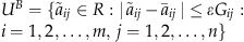, where is the mean or nominal value of , G _ij represents the uncertainty scale particular to the given entry, and ɛ is the uncertainty level common across all the entries (Ben‐Tal et al. 2005). The specific case where corresponds to the case where the relative deviation from the nominal is at most ɛ. That is, for each i and j, lies in the interval . Below, we adopt this case as we focus on the relative uncertainty around positive demand values in our network.

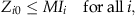
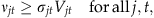
For a constraint i, , we only need to augment the left‐hand side (LHS) of the equation to reflect the uncertainty set in the formulation. Formally, in the augmented constraint we require, for a given solution x, that

Given the structure of U ^B, the optimal solution of the optimization on the LHS is 2 which can be reformulated as 3 4

The constraints (1) are now replaced by (3) and (4), the robust counterpart constraints, and the robust LP is solved.

The box uncertainty set provides a tighter constraint and is thus more conservative than the original (LP). To see this, assume that in problem (LP) for all i, j (the coefficients are at their nominal values). Then the LHS of each constraint (3) is smaller than its counterpart in (LP).

2.1.2. Ellipsoidal Uncertainty

Under ellipsoidal uncertainty, is chosen from a set that expresses a measure of the uncertainty spread. As argued in Ben‐Tal and Nemirovsky (1998, 1999), the box uncertainty set may lead to conservative solutions, as it allows all the uncertain parameters to take on their worst values at the same time. Consider constraint i, , where , i=1, 2, …, m. As an alternative to the box uncertainty set, the uncertain parameters can be characterized by both a nominal vector, , and a positive definite matrix, C _i∈R ^n×n, that expresses the relationship between alternate dimensions of the uncertainty set. Consider the set where Ω_i is a safety parameter indicating the amount of uncertainty, with respect to constraint i, to be covered by the robust solution. Because C is positive definite, the set U _i ^E is an ellipsoid.

For a candidate solution vector x∈R ⁿ, if we restrict uncertain parameters, , to be in the ellipsoid U _i ^E, we have the augmented constraint 5

The LHS of (5) can be solved using the Karush–Kuhn–Tucker conditions to find

Then analogous to the transformation of (2) into (3) and (4), the robust counterpart to the constraint implied by (5) is 6

If one were to assign stochastic uncertainty to the coefficients of matrix A, the solution in (6) suggests that and C _i would represent the expected values, , and the covariance matrix, , respectively, and thus, for a given solution vector, x, one can consider to be a random variable with expected value and standard deviation

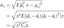
In this case, (6) implies that the constraint holds with Ω_i standard deviations of slack.

In summary, by using an ellipsoid set, we restrict all of the parameters from obtaining their worst‐case values simultaneously. Moreover, if we are to interpret the ellipsoid as representing the mean and covariance structure of the uncertain parameters with a Gaussian distribution, then in the ellipsoidal uncertainty case, the constraints are stochastically guaranteed to a given level through an appropriate choice of Ω.

3. A Multi‐Period Facility Location Problem

In this paper, we consider the application of RO to a capacitated multi‐period fixed‐charge facility location problem. A firm seeks to locate facilities on a connected graph and establish the maximum capacity of these facilities. These decisions are made once at the start of a time horizon and constitute the strategic level decisions of the firm. Then, in each period, the firm observes demand from nodes in the network and must determine how much demand to satisfy and from which facilities. These operational‐level decisions are made subject to the strategic decisions; demand can only be served from open facilities and the total demand served from a facility must be less than its maximum capacity. The firm incurs costs for opening facilities, establishing capacity, producing in a period at a facility, and shipping from a facility to demand nodes. It receives a revenue for each satisfied unit of demand. The objective is to maximize the total system profit.

We assume that the capacity is infinitely divisible and cannot be adjusted during the horizon, though production can be adjusted without cost from period to period. Demand that is fulfilled is done so by direct shipment from a production facility or several facilities to the demand node (i.e., we do not solve for delivery tours). We assume that inventory cannot be carried from period to period. This may be plausible in a service or make‐to‐order firm, as well as in a high volume JIT production environment. However, it is a limitation of the model in an environment where inventory may be built up, e.g., to address seasonal demand.

3.1. Nominal Problem Formulation

We formulate the nominal problem assuming that all data in the problem are deterministic and known, including future demand. Let G(N, A) be a connected graph with nodes and arc set A. Let d _ij be the distance, and, without loss of generality, the cost of shipping units, between nodes i and j for each i, j∈N. We assume d _ij is symmetric and d _ii=0 for all i∈N. Let T be the length of the horizon and D _it, i∈N, t=1, …, T be the demand in period t at node i.

Let K _i be the cost of opening a facility at node i. Let C _i0 be the cost per unit of capacity established at the beginning of the horizon and let c _it be the cost per unit of production at node i in period t. Fulfilled demand generates a revenue of η>0 per unit. Unsatisfied demand is lost. We do not include a discount factor for value over time; one may be readily included.

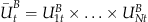
We define the following decision variables: Let I _i=1 if a facility is opened at node i; I _i=0 otherwise. Let Z _i0 be the (maximum) capacity of an open facility at node i. Let X _ijt be the proportion of demand at node j in period t that is satisfied by an open facility at node i (0≤X _ijt≤1). For expositional ease, we also introduce the decision variable Z _it, the production at node i in period t. Finally, let τ be the profit over the horizon. 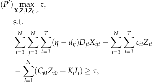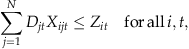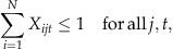The problem is formulated as follows: 7a 7b 7c 7d 7e 7f

Constraint (7a) represents the objective, which is placed in the constraint set to aid the RO formulation below. The first term expresses the revenue less delivery costs; the second term, the production costs; the third, the capacity and facility location cost. Constraint (7b) guarantees the demand satisfied by a facility is less than its production. Constraint (7c) implies at most 100% of the demand at a node is fulfilled. Constraint (7d) ensures that capacity is only available at open facilities. Constraint (7e) implies the production at a facility in each period is less than the established maximum capacity.

If the values of all the parameters were known, problem (P′) could be solved as a mixed integer linear program (MILP) for the optimal strategic decisions and operational decisions. However, if the problem data were uncertain, that solution would not necessarily be optimal. Let , j∈N, t=1, …, T be the uncertain demand at node j in period t. (For simplicity, we consider only demand uncertainty. Other uncertainties such as price, shipping cost, or production cost uncertainty can readily be included.) Using the RO approach, we now reformulate P′ to reflect the allowed uncertainty and solve for both the strategic decisions (location and capacity) and the operational decisions (production and allocation).

3.2. The Robust Problem—Box Uncertainty

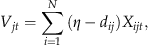
For the case of box uncertainty, we assume that demand in each period is unknown and bounded on a symmetric interval around a known nominal value. That is, let be the uncertain demand from node j in period t and let be its nominal value, i.e., the center point of the interval. Then we assume 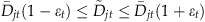for 0≤ɛ _t≤1 for all t, where ɛ _t measures the uncertainty size in period t. We let 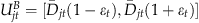, , and . We now transform problem (P′) into a new problem expressing uncertainty by substituting for D _jt in constraints (7a) and (7b) and then augmenting it with the constraint for all j∈N and t=1, 2, …, T.

The augmented constraint for (7a) is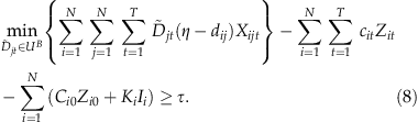

For a given candidate solution X≥0, the optimal solution to the optimization problem on the LHS of (8) is if (η−d _ij)≥0, and if (η−d _ij)<0. However, if (η−d _ij)<0, then X _ijt=0 in the optimal solution to (P′) with (7a) replaced by (8). Thus, we can ignore the second case and find the robust counterpart of constraint (7a) to be 9

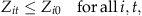
Next, consider constraint (7b) for a given i and t. Noting that the inequality is now “≤,” we augment the constraint by solving for the maximum of the LHS over the uncertainty set, leading to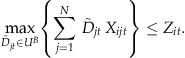

Noting , the constraint implies 10

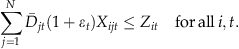
Therefore, the robust counterpart of problem (P′) with uncertainty set U ^B is given by 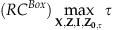subject to constraints (7c)–(7f), (9), and (10).

We let 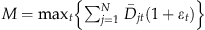be an appropriately large number in (7d). Problem (RC ^Box) is an MILP that can be solved effectively using off‐the‐shelf software.

3.3. The Robust Problem—Ellipsoidal Uncertainty

Consider the case where the uncertain data are contained in an ellipsoid. As discussed in section 2.1 such an ellipsoidal uncertainty set can also be characterized by a mean/variance approach. That is, one can replace the uncertain parameters by their means plus or minus a given number of standard deviations expressing the decision maker's preferences. We define the uncertainty set and then reformulate the robust counterpart of each constraint with uncertain elements in (P′).

As before, let be the uncertain demand at node j in period t. For notational ease, let and be vectors of the demand. Let be the nominal value and let Σ of size (NT×NT) denote the covariance matrix of . (As we assume independence of demands over time and location for our test below, Σ is diagonal with entries σ _ij ².)

Recall in our discussion of the box uncertainty case, the multi‐dimensional unit box was given by the absolute, normalized deviations, i.e.,

To construct the ellipsoid set, we consider the total‐normalized‐squared deviations. Therefore, for the constraint (7a), we define the following uncertainty set: 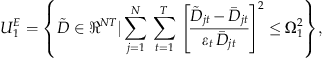11 where Ω₁ is the safety parameter applied to constraint (7a) in (P′). Observe that if we set Ω₁=1 in (11), U ₁ ^E is the largest ellipsoid contained in U ^B, and if we set , U ₁ ^E is the smallest ellipsoid containing U ^B.

Letting and defining Σ to be the NT×NT diagonal matrix with non‐zero entries σ _jt ², then

We now consider the augmented constraint

Let . Similar to (6) we arrive at the robust counterpart constraint 12

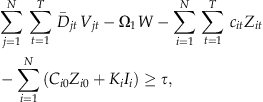
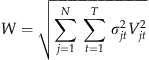
Next, we linearize (12) by considering a decision variable, W, with . This facilitates solution by standard conic optimization (subject to a transformation detailed below). Then the set of constraints 13a 13b 13c form the robust counterpart constraint for constraint (7a) in case of uncertainty set U ₁ ^E.

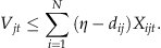
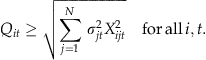
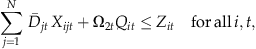
Under the assumption that (the positive orthant), and given the objective of maximizing τ, we can relax (13b) to (13b^\prime) Similarly we can relax (13c) to (13c^\prime)

For each of the constraints (7b), we can also formulate robust counterpart constraints under ellipsoidal uncertainty. Let

Here Ω_2t is the safety parameter associated with the uncertainty in period t. Again we let for each t, and let C _t be the N×N diagonal matrix with non‐zero entries σ _jt ². The augmented constraint for (7b) for a given i and t is

We use a similar approach as in (6) to find the robust counterpart constraint:

Note that we now add in Ω_2t multiples of the uncertainty to reflect the changed direction of the inequality (≤) in (7b). Similar to above, we let 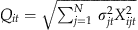. Noting that c _it>0 in the objective function, so that Z _it is to be minimized, we can express Q _it as an inequality, so that the robust counterpart constraints for constraints (7b) are 14 15

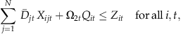
Observe that (13c′) and (15) express conic quadratic constraints. This follows because the variables in their respective vectors [{V _jt}_j, t, W] and [{X _ijt}_j, Q _it] are elements of Lorentz cones, i.e., [{V _jt}_j, t, W]∈L ^NT+1 and [{X _ijt}_j, Q _it]∈L _it ^N+1, where L ^y is the Lorentz cone of dimension y. Note, however, that variable X _ijt appears in L _it ^N+1 and, because of (13b), also in L ^NT+1. This proves problematic in solving the resulting conic optimization problem. Therefore, we define ν _jt≥σ _jt V _jt for all j and t, and χ _ijt≥σ _jt X _ijt for all i, j, and t. We then replace (13c′) by 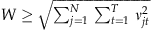and (15) by 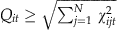. The complete robust counterpart of (P′) is 16a 16b 16c 16d 16e 16f (16g) and constraints (7c)–(7f).

Here we let M in (7d) be sufficiently large, e.g., M=N max_j,t[D _jt∈U ^E].

In this formulation when we consider the demand revenues in (16a), the uncertainty expresses the possible downside of lower than expected revenues. In doing so, we limit the overall uncertainty in all periods under consideration through the summation in (16f). In comparison, when considering the production required in (16b), the uncertainty expresses the alternate downside of high requirements for capacity. In this case we limit the demand required to be served in each period separately through (16g). The effect of these is similar to the box uncertainty case—we require sufficient capacity in each period to serve the demand expected, but assume lower revenues in finding our profits than would be implied by these high demands.

Problem (RC ^Ell) is a conic quadratic program. There are several software programs that efficiently solve conic quadratic programs, e.g., the MOSEK optimization tools—http://www.mosek.com. We note that problem (RC ^Box) has N ² T+N(T+2)+1 variables, of which N are binary, and N(3T+1)+1 constraints. Problem (RC ^Ell) has 2N ² T+N(4T+2)+2 variables, of which N are binary, and N ² T+N(6T+1)+2 constraints, of which NT+1 are conic quadratic constraints. This increase in the number of variables and constraints heavily impacts the size of the mixed‐integer problems that can be solved. We turn next to solving examples of these programs to evaluate how the alternate robust models affect the objective value and the solutions.

4. Numerical Study

In this section, we conduct numerical experiments to understand how the solutions provided by the nominal problem and the RO models, using either box or ellipsoidal uncertainty sets, differ. We consider how they differ in the number of facilities opened, their capacities, and the network topology determined by the solution. In addition, we study the expected profit under each model as given by a simulation of demand sample paths. Before presentation of the results, we describe the test environment in detail.

4.1. Test Environment

We randomly generate N nodes on a unit square, representing the demand points and potential facility locations. The nominal demand at each demand point in each period, , is independent of all others and is assumed constant over the T periods. We let N=15 and T=20. The nominal demand at each location is drawn from the uniform distribution, Uniform [17,500, 22,500].

We use the revenue and cost parameters summarized in Table 1 for the base case. The revenue is set at η=1. The delivery cost, d _ij, equals the Euclidean distance between nodes i and j. The expected distance between any two nodes is approximately 0.5 and the expected maximum distance is approximately 1 (see, e.g., Larson and Odoni 2007). We let C _i0=0.1, c _it=0.1 (∀i, t) and K=50,000. Using these values, the expected margin per unit per period is approximately 0.3 if one location is opened and 0.9 if all N locations are opened. The cost of opening a facility to serve the average demand is approximately between 3 and 10 periods of demand.

Table 1

Parameter Values in Base Case

η	1
N	15
T	20
c _it	0.1
C _i0	0.1
K	50,000
D _j	∼U[17500, 22500]

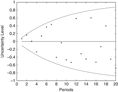
The initial uncertainty sets are generated as follows. In the base case we let γ=0.15 be the initial (first period) uncertainty in the demand, and let ɛ _t=γ+(1−γ)ɛ _t−1 with ɛ ₀=0. For the box uncertainty set we assume . Because ɛ _t is a concave, increasing function in t, U _jt ^B is increasing in t. In Figure 1, the solid lines depict the boundaries of U _jt ^B. The marked points depict a sample path that might occur (described below). For the ellipsoidal uncertainty set we let the safety parameters Ω₁ and Ω_2t for t=1, …, T equal 1. This creates the largest ellipsoid contained in the box U ^B (the inscribed ellipsoid).

Figure 1

Box Uncertainty Set given by γ=15% and an Instance of a Sample Path in the Box

We compare the solutions of the nominal problem to those of the box and ellipsoidal uncertainty problems. We do so by first considering the topology of the solutions (number of facilities established, number of edges utilized, etc.). Second, we compare the profit of the solutions found.

4.2. Comparing the Topology of the Solutions

We compare the number of facilities opened, the capacity of the facilities, and the connectivity of the graph for the three models. To do so, we generate 250 random graphs by choosing node locations uniformly over the unit square. For each graph we solve the nominal, box uncertainty, and ellipsoidal uncertainty models. For each graph we generate 10 sample paths for the demand for a total of 2500 sample paths. The sample paths are generated by sampling over the box uncertainty set for each time period t (the area between the curves in Figure 1). Sampling is conducted using either a bell‐shaped beta(2, 2) distribution, uniform distribution, or U‐shaped beta(1/2, 1/2) distribution.

In Figure 2, we present typical solutions of the models. In the figures, a star denotes an open facility (co‐located with a demand node), a circle represents a demand node, and a line indicates that in at least one period the facility is used to satisfy demand at the node. The size of the stars is proportional to the capacity of the facility. In Table 2, we present the mean number of facilities, mean capacity, and mean number of connections per open facility. The last is defined as 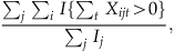where I{} is the indicator function. We also present the percentage of the demand covered by each of the three solutions. Results are given for the case of η=1, 3, and 6.

Figure 2

Network Representations of the Solution to an Instance of (a) the Nominal Model, (b) Box Uncertainty Case, (c) Ellipsoidal Uncertainty Case

Table 2

Comparing the Solution Topology of the Three Models

	Model	Mean # of open facilities	Mean capacity	Mean # edges/facility	% of demand covered
	Model	Mean # of open facilities	Mean capacity	Mean # edges/facility	Uniform	Bell‐shape	U‐shape
η=1	Nominal	10.74	28,221	0.42	96.99	94.99	94.58
	Box	3.48	140,350	3.91	100	100	100
	Inscribed ellipsoid	8.68	59,737	14.36	100	100	100
η=3	Nominal	10.74	28,221	0.42	96.74	95.08	94.62
	Box	4.24	136,425	3.25	100	100	100
	Inscribed ellipsoid	8.66	59,822	14.34	100	100	100
η=6	Nominal	10.74	28,221	0.42	96.74	95.08	94.62
	Box	4.44	134,485	2.94	100	100	100
	Inscribed ellipsoid	8.66	59,759	14	100	100	100

We make several observations. First, compared with the nominal model, both robust models with the box and ellipsoidal uncertainty sets open fewer facilities with larger capacities, with the box model opening far fewer. Because the box uncertainty set contains the ellipsoid set, the degree of uncertainty is greater in the former. Therefore, it must respond simultaneously to both higher potential demand (resulting in larger capacity) and lower potential revenue (resulting in fewer facilities, lowering the fixed cost). As such, we find the strategic cost (the initial cost of establishing the facilities and their capacities) for the box uncertainty model to be 40% of the cost in the nominal model. In comparison, the ellipsoidal model strategic cost is 90% of that of the nominal model. Second, the ellipsoidal uncertainty model establishes more edges per open facility than the nominal model. Importantly, it allows more than one facility to serve the same demand node, expressing flexibility in the service to increase robustness to demand uncertainty. This stands in contrast to both the nominal and box uncertainty models that almost always serve each demand node from a unique facility. Finally, we observe that on the sample paths, the two robust models cover 100% of the demand compared with 95% for the nominal model. This indicates the robust models are performing as expected in terms of their ability to address uncertainty.

4.3. Comparing the Profit of the Solutions

In this subsection, we compare the profit of the robust models to that of the nominal model as we change various parameters of the model. For each of the models, we solve the associated mathematical programs for I _i, Z _i0 (the strategic decisions of location and capacity), and for Z _it, and X _ijt (the operational decisions of production and allocation). In practice, however, while the firm cannot change the strategic decisions under our assumptions, it will, upon observation of demand, determine the active operational decisions, say and . That is, given a solution, and , for each period t, we assume the firm observes realized demand and solves the following operational problem for the operational profit, Π_t:

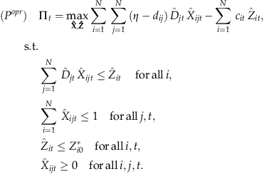
We compare the performance of the strategic solutions with respect to sample paths for the uncertain demand. To do so, we generate sample paths for the demand at the demand nodes and then optimize (P ^opr) for the operational decisions and for each of the models using the bell‐shaped, uniform, and U‐shaped distributions. This allows us to estimate the operating costs associated with the strategic solution. Throughout these tests, we consider a single‐network topology (the location of facilities). The nominal demand for the base case in the tests is 20,000 units per period for each node (as opposed to sampled from the range [17,500, 22,500]). All other parameters are as given in Table 1. For each of the distributions, we generate 1000 sample paths.

First, we consider how the base case box and ellipsoidal uncertainty robust models perform as the nominal demand grows for the various demand distributions. Second, we consider the trade‐off between robustness of the solution and performance vs. the nominal solution. Third, we vary the horizon length. Finally, we vary the fixed charge.

4.3.1. Profit vs. Demand Growth and Uncertainty

In Table 3, we present the percentage increase (or decrease) in the profit for the base case box and ellipsoidal uncertainty models relative to the nominal model. We do so for the case with constant nominal demand and two cases where the nominal demand increases: demand growing by 500 units per period (a 2.5% growth rate) and demand growing at 1000 units per period (a 5% growth rate). We also present the standard deviation of the increase in profits. In addition, for each sample path, we solve for the optimal solution of the nominal problem, (P), with the demand determined by the realized sample path. Doing so provides an upper bound on the possible profit achieved. We present the percentage of the difference between the upper bound and the nominal solution given by the solution value (UB). That is, (solution value−nominal)/(upper bound−nominal). For example, in the box uncertainty case when demand is uniformly distributed over the uncertainty set, we observe a 1.65% increase in average profit, which corresponds to achieving 17.29% of the possible increase in the profit. Alternately, if the demand was drawn from a bell‐shaped distribution, there is a decrease of 0.48% in the average profit and thus does not correspond to any percentage increase.

Table 3

Percentage Increase in Profit over the Nominal Model, Associated Standard Deviations and Implied Percentage of Upper Bound Achieved for the Base Case Box and Inscribed Ellipsoidal Uncertainty Models

Case	Box uncertainty			Inscribed ellipsoidal uncertainty
Case	Bell	Uniform	U‐shape	Bell	Uniform	U‐shape
Base case
Mean %	−0.48	1.65	3.77	6.12	8.28	10.34
Standard deviation	0.98	1.20	1.61	1.16	1.43	1.89
% of upper bound	<0	17.29	34.69	93.03	95.59	96.47
Growth +500 ×t
Mean %	−5.18	−3.71	−2.16	2.15	3.72	5.49
Standard deviation	0.67	0.78	0.95	0.80	1.03	1.35
% of upper bound	<0	<0	<0	66.86	78.12	85.15
Growth +1000 ×t
Mean %	−7.41	−6.44	−5.39	1.43	2.85	4.42
Standard deviation	0.41	0.51	0.62	0.74	1.00	1.26
% of upper bound	<0	<0	<0	54.19	72.03	81.33

We observe that the (inscribed) ellipsoidal uncertainty case provides significantly better solutions to the operational problem faced than that of the nominal or box uncertainty cases. This result is not surprising as it emphasizes the difference in the nature of the solutions between the two robust models. The box is defined to immunize the solution against any possible outcome within the assumed uncertainty set, whereas the inscribed ellipsoid does not immunize the solution against realizations in the corners of the box. For the demand distributions, we test under the assumption of independent sampling; the inscribed ellipsoid immunizes the solution against realizations more likely to happen. Thus, the box model adopts a very conservative approach, establishing centralized facilities that can be deployed to meet any demand. However, the ellipsoidal model establishes multiple, flexible facilities, close to those given by the nominal solution, but sized to address potential uncertainty. From a sample path standpoint, such a model appears to have better performance. On average, the ellipsoidal model captures 80.3% of the benefit possible as given by the upper bound.

We observe that the best performance for each case (both in mean profit and percentage of upper bound) is when expected demand is constant over time. When there is a trend in the growth over the period (either at 500 or 1000 per period), the benefit of both RO models diminishes. In the box uncertainty model, in each of the demand growth cases, the performance is worse than the nominal model, though that of the ellipsoidal model is still positive. Further, as would be expected, both RO models perform better as the likelihood of more extreme demand increases, i.e., as the sampling distribution changes from a bell‐shaped to uniform to U‐shaped distribution.

4.3.2. Robustness–Performance Trade‐Off

As we observe above, the model with the ellipsoidal uncertainty set finds a solution that performs better than the model with the box uncertainty set that circumscribes it, even when the actual demand is drawn from a distribution with support over the entire box. Again, this is not surprising as the solution for the ellipsoid case does not immunize the solution against all of the uncertainty contained in the box. Next, we investigate how by assuming a smaller uncertainty set (either for the box or the ellipsoid models) one can find a better performing solution. That is, we will immunize the solution against a smaller uncertainty set; however, in testing we continue to sample from the base case box uncertainty set.

Consider first the box model. In the base case, we assumed the box was defined by an initial uncertainty γ=0.15, and then defined ɛ _t for t=1, …, i. Suppose that we vary the value of γ, and therefore ɛ _t, to define a new box uncertainty set. Let ρ be the ratio of the volume of the box uncertainty set to the volume of the base case box, i.e., ρ=100% in the base case. For each value of ρ, we can also generate an ellipsoid that is equal in volume to that specific box. To do so, as above, we let as ɛ _t varies. Then, rather than using the inscribed ellipsoid, by properly scaling the safety parameters Ω₁ and Ω_2t we equate the multi‐dimensional volumes of the box and ellipsoid. For the base case with N=15 nodes and T=20 periods, we find Ω₁=8.4784 and Ω_2t=2.1327 (see chapter 2 of Ben‐Tal et al. 2009 for details on such scaling). Observe this ellipsoid is larger than the inscribed ellipsoid defined by Ω₁=Ω_2t=1.

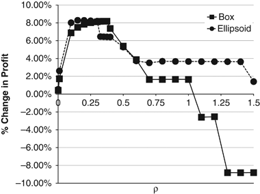
In Figure 3, we plot the percentage increase (relative to the nominal model) in the robust solution profit as we vary ρ from 0.1% to 150% assuming the demand is sampled uniformly over the base case box uncertainty set. We observe that the box model's maximum improvement is approximately 8.18% at approximately ρ=0.35, and the ellipsoid model's is approximately 8.28% at ρ=0.15. The “best” ellipsoid captures infrequent, but potentially important, demand observations toward the edges of its volume. Intuitively, for the box to do the same it would need to be larger; thus, the larger volume of the “best” box. For smaller ρ, the robust models do not immunize the solution against much uncertainty and therefore perform close to the nominal model. For larger values of ρ, the performance decreases as the models increasingly immunize the solution against uncertainties that are unlikely to occur. In particular, we observe an expected profit loss for the box case for ρ>100%, i.e., for boxes larger than the base case from which demand is sampled, there is no longer a trade‐off; greater robustness only results in lowered profits. The results indicate that for small ρ both models can balance robustness with profits.

Figure 3

Percentage Increase (Relative to the Nominal Model) in Profit for Models with Box and Ellipsoid Uncertainty Sets, as the Value of ρ Changes

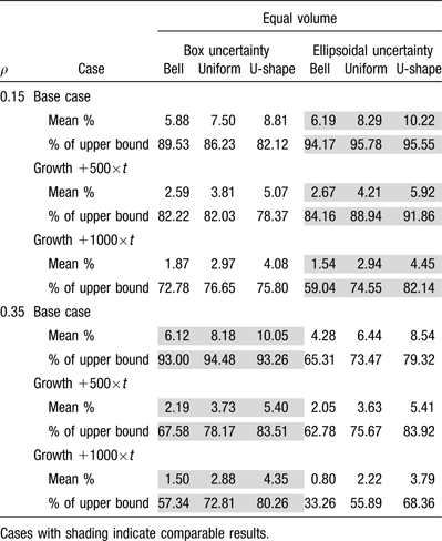
In Table 4, we present the results for the box and ellipsoid models for ρ=0.15 and ρ=0.35, corresponding roughly to the best performance for each model. We note the similarity of the ellipsoid model at ρ=0.15 to the box model at ρ=0.35 (shown in the shaded regions in the table). Also note the similarity to the ellipsoid inscribed in base case box, given in Table 3. That is, the inscribed ellipsoid performs very nearly as well as the best possible ellipsoid, at least for the test case. As above, the performance for each model increases as the demand spreads away from the mean (U‐shaped vs. bell‐shaped), and decreases as the rate of demand growth over time increases. We note that in all these cases the ellipsoid performs slightly better than the box model.

Table 4

Percentage Increase in Profits over the Nominal Model and Implied Percentage of Upper Bound Achieved for the ρ=0.15 and ρ=0.35 Cases

4.3.3. Varying Horizon Length, T

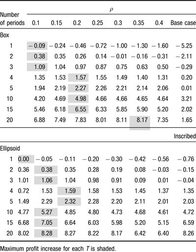
We investigate how the robust solutions compare with the nominal solution as the length of the horizon changes. Results are reported in Table 5. We present the box and ellipsoid models for ρ∈[0.1, 0.4], the base case (ρ=1.0), and the inscribed ellipsoid for the base case. Increase in profit is reported vs. the nominal with uniform sampling over the base case box. We observe that for a given ρ, as the number of periods increases, the profit increases vs. the nominal for both the box and ellipsoidal cases (with the exception of ρ=1). This result is similar to that of Bertsimas and Thiele (2006). In the table, we emphasize the best performance for each horizon length for the two models. We observe that as the horizon increases, a larger box uncertainty set is required to achieve better performance, while an ellipsoid with ρ=0.15 is almost always the best value. Further, we observe that for the higher number of periods, the ellipsoidal model performs better than the box at their respective maxima. The flexibility provided by the ellipsoidal uncertainty model at ρ=0.15 allows the firm to find solutions that can better accommodate greater variation in the demand found over a longer horizon, whereas the box size must increase.

Table 5

Percentage Increase in Profit for Box and Ellipsoidal Uncertainty Sets when Varying T

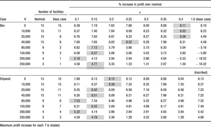
4.3.4. Varying Fixed Cost, K

We explore the effect of changing the fixed cost K in Table 6. We highlight the best performance for the various values of ρ for each model. For smaller fixed costs, the box model's results are better for larger ρ. As in Table 5, the ellipsoid model best performance is generally close to ρ=0.15, which is also similar to the performance of the inscribed ellipsoid for ρ=1. Observe that as the value of K increases, the number of facilities opened decreases. For comparison purposes, we present the number of facilities opened in the nominal, base case box (ρ=1), and inscribed ellipsoids in the table. As in section 4.2, the base case box opens fewer (and larger) facilities than the robust model with the inscribed ellipsoid. We find that only a limited amount of uncertainty should be addressed, roughly comparable to that of the inscribed ellipsoid. As before, we find the value of ρ=0.15 robust in doing so for the ellipsoid. For the box, by reducing the uncertainty set, more facilities are opened and the benefits of flexibility are gained.

Table 6

Number of Open Facilities and Percentage Increase in Profit for Box and Ellipsoidal Uncertainty Sets Varying K

5. Discussion

The objective of this paper is to investigate potential means by which RO techniques could be used to solve facility location problems. Previous work on RO has not considered such problems, particularly our approach to profit maximization. The results of the work reemphasize the need to evaluate the nature of the uncertainty allowed. We show that the alternate models of uncertainty lead to very different solution network topologies with the box uncertainty case opening fewer, larger facilities. We then generate sample paths in order to test how the alternate solutions to the strategic problem would perform in practice. For each sample path, we solve the resulting operational problem of determining production and allocation. We find that the robust model with the box uncertainty performs poorly with respect to balancing robustness with profit. In contrast, the model with the inscribed ellipsoid provides small but significant improvements in the average profit. We show, however, similarly good results are obtained by varying the size of the box or ellipsoid used to immunize the solution against uncertainty. Importantly, we find that a single ellipsoid is able to provide good solutions over a wide range of parameter choices.

The problem we solve is difficult as it is a mixed‐integer conic program. Within our problem formulation, demand appears in two places: first, as a multiplier for the revenues determining the objective function value, and second as a multiplier for the production capacity for each of the nodes. As such, these lead to alternate requirements of the solution; namely, the ability to address large demands, while at the same time observing low revenues. The resulting conic quadratic program for the ellipsoidal case is large by the standards of conic programming (up to 20 periods and 15 nodes). While such a problem may be considered to be of only semi‐realistic size, we emphasize that other methods, particularly stochastic programming, would have great difficulty in solving problems of such size.

We find the solutions given by the robust model with ellipsoidal uncertainty set address the need for robustness directly by considering alternate links between facilities and nodes to accommodate the uncertain demand. Future work may consider additional uncertainty sets such as a polyhedra, e.g., an intersection of box with an L ₁ norm. These may prove to provide solutions to larger problems while restricting the uncertainty away from worst‐case scenarios.

Footnotes

Acknowledgments

Support for this research was provided by grants from the Natural Science and Engineering Research Council of Canada. The authors would like to thank the journal's editorial team for their many helpful suggestions.

References

Adida

Perakis

. 2006. A robust optimization approach to dynamic pricing and inventory control with no backorders. Math. Progrm., Ser. B 107 (1–2): 97–129.

Averbakh

Berman

. 1997. Minimax regret p‐center location on a network with demand uncertainty. Locat. Sci. 5 (4): 247–254.

Averbakh

Berman

. 2000a. Algorithms for the robust 1‐center problem on a tree. Eur. J. Oper. Res. 123 (2): 292–302.

Averbakh

Berman

. 2000b. Minimax regret median location on a network under uncertainty. INFORMS J. Comput. 12 (2): 104–110.

Ben‐Tal

El‐Ghaoui

Nemirovsky

. 2009. Robust Optimization. Princeton University Press, Princeton, NJ.

Ben‐Tal

Golany

Nemirovsky

Vial

J‐P.

. 2005. Retailer‐supplier flexible commitments contracts—a robust optimization approach. Manuf. Serv. Oper. Manage. 7: 248–271.

Ben‐Tal

Margalit

Nemirovsky

. 2000. Robust modeling of multi‐stage portfolio problems. Frenk

Roos

Terlaky

Zhang

, eds, High‐Performance Optimization. Kluwer Academic Publishers, Dordrecht, The Netherlands, 303–328.

Ben‐Tal

Nemirovsky

. 1998. Robust convex optimization. Math. Oper. Res. 23 (4): 769–805.

Ben‐Tal

Nemirovsky

. 1999. Robust solutions of uncertain linear programs. Oper. Res. Lett. 25 (1): 1–13.

10.

Berman

Wang

. 2006. The 1‐median and 1‐antimedian problems with continuous probabilistic demand weights. INFOR 44: 267–283.

11.

Bertsimas

Pachamanova

Sim

. 2004. Robust linear optimization under general norms. Oper. Res. Lett. 32 (6): 510–516.

12.

Bertsimas

Sim

. 2006. Tractable approximations to robust conic optimization problems. Math. Program., Ser. B 107 (1–2): 5–36.

13.

Bertsimas

Thiele

. 2006. A robust optimization approach to inventory theory. Oper. Res. 54 (1): 150–168.

14.

Carrizosa

Nickel

. 2003. Robust facility location. Math. Methods Oper. Res. 58 (2): 331–349.

15.

Chen

Daskin

M. S.

Shen

Z.‐J. M.

Uryasev

. 2006. The α‐reliable mean‐excess regret model for stochastic facility location modeling. Nav. Res. Logist. 53 (7): 617–626.

16.

Cohen

Golany

Shtub

. 2007. The stochastic time‐cost tradeoff problem: A robust optimization approach. Networks. 49(2): 175–188.

17.

Daskin

1995. Network and Discrete Location: Models Algorithms and Applications. John Wiley and Sons, New York.

18.

Daskin

M. S.

Coullard

C. R.

Shen

Z. M.

. 2002. An inventory‐location model: Formulation, solution algorithm and computational results. Ann. Oper. Res. 110 (1–4): 83–106.

19.

Daskin

M. S.

Hesse

S. M.

ReVelle

C. S.

. 1997. α‐reliable p‐minimax regret: A new model for strategic facility location modeling. Locat. Sci. 5 (4): 227–246.

20.

Drezner

Hamacher

. 2002. Facility Location: Applications and Theory. Springer, Berlin.

21.

El‐Ghaoui

Lebert

. 1997. Robust solutions to least‐square problems to uncertain data matrices. SIAM J. Matrix Anal. Appl. 18 (4): 1035–1064.

22.

El‐Ghaoui

Oustry

Lebert

. 1998. Robust solutions to uncertain semidefinite programs. SIAM J. Optim. 9 (1): 33–52.

23.

Gutierrez

G. J.

Kouvelis

. 1995. A robustness approach to international sourcing. Ann. Oper. Res. 59 (1): 165–193.

24.

Kouvelis

Kurawarwala

A. A.

Gutierrez

G. J.

. 1992. Algorithms for robust single and multiple period layout planning for manufacturing systems. Eur. J. Oper. Res. 63 (2): 287–303.

25.

Larson

R. C.

Odoni

A. R.

. 2007. Urban Operations Research. Dynamic Ideas, Belmont, MA.

26.

Louveaux

F. V.

1986. Discrete stochastic location models. Ann. Oper. Res. 6 (2): 23–34.

27.

Mirchandani

P. B.

Francis

R. L.

. 1990. Discrete Location Theory. John Wiley and Sons, New York.

28.

Mirchandani

P. B.

Oudjit

Wong

R. T.

. 1985. Multidimensional extensions and a nested dual approach for the m‐median problem. Eur. J. Oper. Res. 21 (1): 121–137.

29.

Snyder

Daskin

M. S.

. 2006. Stochastic p‐robust location problems. IIE Trans. 38 (11): 971–985.

30.

Snyder

L. V.

2007. Facility location under uncertainty: A review. IIE Trans. 38 (7): 537–554.

31.

Snyder

L. V.

Daskin

M. S.

Teo

C.‐P.

. 2007. The stochastic location model with risk pooling. Eur. J. Oper. Res. 179 (3): 1221–1238.

32.

Soyster

A. L.

1973. Convex programming with set‐inclusive constraints and applications to inexact linear programming. Oper. Res. 21 (5): 1154–1157.

33.

Verter

Dincer

M. C.

. 1992. An integrated evaluation of facility location capacity acquisition and technology selection for designing global manufacturing strategies. Eur. J. Oper. Res. 60: 1–18.

34.

Weaver

J. R.

Church

R. L.

. 1983. Computational procedures for location problems on stochastic networks. Trans. Sci. 17 (2): 168–180.