Optimal Enhancement and Lifetime of Software Systems: A Control Theoretic Analysis

Abstract

We develop an optimal control model to maximize the net value provided by a software system over its useful life. The model determines the initial number of features in the system, the level of dynamic enhancement effort, and the lifetime of the system. The various factors affecting these optimal choices are systems characteristics (e.g., complexity, age, quality), user learning, and process maturity. We also consider that there is a time lag between the addition of a feature and the realization of its benefit to users. The basic model is extended to consider the decision of replacing the existing system by a new one.

Keywords

software enhancement lifetime features replacement optimal control theory

1. Introduction

The widespread adoption of information technology over the past few decades has created new challenges of delivering software systems with new features. Software systems are among the most complex artifacts produced by humans. This complexity arises not only due to the inherent complexities of the product, but also due to difficulties in managing the software development process. Our focus in this study is on managing the capabilities of a software system over its useful life.

A study by Whittaker (1999) finds that more than half of software development projects cost an average of 89% over the original estimate. Hence, in an effort to control costs while providing sufficient organizational value, firms explore various strategies to manage the software development and enhancement process. We contribute to the software system management area by proposing an analytical model to determine the optimal number of features in a software system when it is initially put to use as well as the enhancement effort that must be applied during its life.

1.1. Problem and Motivation

One important distinction between software and physical goods is that adding features to a software product is relatively easier than it is to a finished physical good. For example, adding features to an automobile or an electronic item may require several costly and time‐consuming design changes (Boothroyd et al. 2002, Lehman and Ramil 2002), whereas features may be added to a software product incrementally (Cusumano and Selby 1997). In the software industry, each new release of a product builds on the past releases by adding new features to the current code base. This multiple‐release development strategy operates across most common software products—from operating systems (e.g., Mac OS, Windows, DOS) to different application systems (e.g., Microsoft Excel, Matlab, Stata) (Rahmandad 2005). Another real‐world example is the software system in the online invoicing company SimplifyThis.¹ The initial features in its software included features such as “sending an invoice to customers electronically,”“receiving payments electronically,” etc. Later, new features such as “time tracking on projects,”“integrating customer account pages,” etc., were added during the enhancement (S. Kumar, personal communications).

The software industry is estimated to reach US$2 trillion by 2008 (Heineman and Councill 2001). In this fast growing and rapidly changing environment, users are demanding more capabilities (features) in software products. US companies spend more than US$70 billion annually on the maintenance and enhancement of software (Sutherland 1995). Large organizations usually allocate 50–80% of their information systems department budget to enhance their existing software (Banker et al. 1991, Eastwood 1993, Lientz et al. 1978). Swanson and Beath (1989) report that the attention of organizations is shifting from new application development to the maintenance and enhancement of currently installed systems. Organizations are faced with the problem of continually enhancing existing software systems, quickly and at low cost (Rahmandad 2005). We address this problem by developing a dynamic model, arising from the need to dynamically enhance a software system if it is to continue to benefit the organization that deploys it (Lehman and Ramil 2002).

We consider an organization that can enhance a software product while it is in use. In the case of in‐house developed software, organizations typically have this ability because they are likely to be familiar with the software's internal structure and code. Even for some commercial off‐the‐shelf (COTS) software systems, software vendors may share the source code with customers due to legal and competitive reasons. For example, Microsoft had to disclose portions of the Windows source code to nine states and the District of Columbia because of litigation (Wilcox 2002a). Real Networks disclosed its software blueprint in an effort to compete with Microsoft (Wilcox 2002b). Finally, in the case of open‐source software, complete access to the source code is available. Our proposed model is therefore applicable in all the above situations where the organization has the ability to enhance an existing software system.

Software systems usually have a limited life because, after a certain time, the cost of maintaining them exceeds the value they generate. Hence, in the last stage of a software life‐cycle, referred to as the close‐down stage, the software is withdrawn, and there may be another stage before that, called the phase‐out stage, where no effort is made to enhance the system (Rajlich and Bennett 2000). It is a critical decision for an organization to optimally determine the phase‐out and close‐down stages with a view to maximizing net benefit over the period of use. Although the significance of this problem is discussed by several practitioners and researchers (Banker and Slaughter 2000, Lientz et al. 1978), no formal analysis has been provided. The model in this paper fills this gap by also finding the optimal phase‐out and close‐down times together with the enhancement effort that must be applied before the start of phase‐out.

In addition to the above considerations, a new software system may become available for adoption while the existing system is being used. In these situations, the organization has the option of replacing the system even before the close‐down stage (Chan et al. 1996, Sneed 1995). We extend our model to consider this scenario where the organization simultaneously optimizes the following: (i) the enhancement effort for the current system, (ii) the effort on learning the new system, and (iii) the time to upgrade to the new system.

1.2. Objective and Contributions

The main goal of this study is to optimally manage the life‐cycle decisions of a software system. There are three important decisions to be made: choosing the optimal number of features at the time of adoption, choosing the optimal effort level to add more features after its adoption, and optimizing the lifetime of the system. Clearly, these three decisions are interrelated, and cannot be optimized separately. We therefore develop an optimal control model to optimize these decisions simultaneously.

The objective in this model is to maximize the total discounted profit over the lifetime of a software system. The profit rate at any instance of time includes the benefit rate as well as the various cost rates incurred at that time. A novel aspect of our model is the inclusion of a time lag between the addition of a feature to the system and the realization of its benefit. Such time lag has mainly been ignored by the extant research, except for a few studies such as Gaimon (1997) and Carrillo and Gaimon (2000). We also allow for the fact that the benefit of adding a feature is higher for users if they have more experience with the system. This “learning‐by‐doing” impact on benefit has been observed, e.g., by Arrow (1962) and Schilling et al. (2003).

The increase in the number of features at any time depends on the effort level at that time as well as the effectiveness of the effort. As observed in the past studies (Ji et al. 2005, Kafura and Reddy 1987, Lehman 1980, Lehman and Ramil 2002, Mookerjee and Chiang 2002), the effort becomes less effective as the complexity of the system increases. This impact of complexity on the effectiveness of enhancement effort is explicitly incorporated in our model.

Another important aspect of our model is that it considers the cost of fixing new bugs that may inadvertently be injected into the existing system with the addition of new features. We illustrate this possibility using the previous example of SimplifyThis. With the addition of new features, the contextual menus in the customer and project sections of the system stopped working correctly on some browsers (S. Kumar, personal communications, SimplifyThis 2008). SimplifyThis had to put in considerable additional effort to fix this bug.

The following three factors usually impact the number of bugs injected during enhancement and the cost of fixing them: (a) the number of new features added to the system (Lanning and Khoshgoftaar 1995), (b) the complexity of the system (Banker et al. 1993, Lehman and Ramil 2001), and (c) familiarity of developers with the system (Harter and Slaughter 2003). We consider these factors while modeling the cost of fixing bugs.

It is common to characterize software maintenance as consisting of three types of activities (Lientz et al. 1978, Swanson 1976). Briefly, these activities are corrective maintenance (performed in response to occurrence of failures), adaptive maintenance (performed in anticipation of changes within the data or processing environment), and perfective maintenance (performed to eliminate inefficiencies and enhance performance). In practice, organizations usually combine perfective and adaptive maintenance activities under the term enhancement (Couger and Colter 1985, Swanson and Beath 1989). We therefore refer to the combination of these two types of maintenance activities as enhancement. In addition to software enhancement, the organizations also need to perform corrective maintenance throughout the system lifetime. In our model, we refer to corrective maintenance as simply maintenance. Past research focuses on the system enhancement mainly as response to external events, such as enhancement requests by users (Feng et al. 2006, Tan and Mookerjee 2005). Instead, we consider the enhancement decision as endogenous, driven by economic factors (benefits and costs).

We solve an optimal control problem developed on the lines discussed above and present a closed‐form solution. This solution affords several managerial insights. We find that when the initial number of features in a released system is below a threshold, then maximum enhancement effort should be spent in the beginning. On the other hand, if the initial number of features in a released product is above that threshold, then the organization should not put any effort to enhance the product right after its release, because the marginal benefit from adding features at that time is less than its cost. However, as discussed earlier, the value of adding features increases with user experience. Therefore, it becomes more beneficial to add features after a certain time has elapsed. However, because it takes time to learn new features (learning lag), new features should not be added near the end of the lifetime of the software.

Further, we optimally choose the initial number of features and investigate the impact of the learning lag on (i) the initial number of features, (ii) the net enhancement value, (iii) the amount of improvement from using the optimal solution as compared with the solutions from two sub‐optimal, but intuitive policies, and (iv) the regions for maximum‐growth (of features), steady‐growth, and no‐growth. As the learning lag increases, the initial number of features increases and the amount of net enhancement decreases. As the strength of optimal solution lies in optimizing the enhancement effort, the improvement from using the optimal solution (over other sub‐optimal policies) diminishes with an increase in the learning lag. Also, with an increase in learning lag, the time regime for no‐growth expands whereas the time regime for maximum‐growth and steady‐growth shrinks. Hence, the total time for enhancement reduces with an increase in learning lag.

Next, we extend our model to consider replacement: a scenario where a new system is available for adoption while the existing system is being used. In this model, we optimize the enhancement and upgrade decisions simultaneously. Our analyses show that the time at which the new system becomes available (T) has a crucial impact on the enhancement strategy when the new system is highly valuable (compared with the existing system) and the enhancement cost is moderate. Hence, in this region, it is important to estimate accurately when the new system would become available. In other regions, it is not worthwhile to spend much effort in accurately estimating T. We investigate the impact of the value of the new system and the cost of fixing bugs on the optimal number of initial features and the enhancement and upgrade strategies. Our results show that it is important to estimate the value of the new system accurately because the optimal strategy reverses when the value of the new system exceeds beyond a given threshold.

Some practitioners and researchers advocate a fixed‐allocation policy where the amount of enhancement effort is constant during the system lifetime for ease of management (McConnell 1997). Hence, we compare this policy with the optimal policy. It is very useful for the managers to evaluate the relative advantage of using the optimal policy. It is also not unusual to find organizations which perform only the corrective maintenance for the released product, and not the perfective and adaptive maintenances (i.e., enhancement). Therefore, we also include a policy for comparison where organizations do not allocate any enhancement effort. We refer to this policy as the maintenance‐only policy. The insights presented in this paper based on these analyses would help managers in finding the optimal policy as well as guide them in making strategic and tactical decisions over time.

The rest of the paper is organized as follows. We briefly review the additional related literature in section 2. The detailed model for the single software system is provided in section 3. In section 4, we present the optimal solution and the analysis of the results. In section 5, we consider the possibility of replacing the old system with a new one. In section 6, we present a numerical study and provide managerial insights. Section 7 concludes the paper and discusses future research directions.

2. Literature Review

Software development research can be broadly classified into two streams. The first is concerned with decisions faced by a software development team before a software product is released. Previous works in the first stream address the issues related to the construction, integration, and testing (while the software is being developed), and the release time of the software. The earlier software development practices prescribe that integration, testing, and debugging be performed only after the construction is completed. In this direction, Koushik and Mookerjee (1995) model the coordination process in the construction phase with the objective of minimizing the coordination effort subject to the constraint that the system is completed within a specified time period. The problem of optimally sequencing the creation of elements in a project is studied by Liu et al. (2007).

In the 1990s, large software vendors, such as Microsoft, started advocating the idea of the synch‐and‐stabilize approach—continually synchronize what people are doing as individuals and as members of parallel teams, and periodically stabilize the product in increments as the project proceeds, rather than once at the end of the project (Cusumano and Selby 1997). This concept is similar to the idea of concurrent engineering in manufacturing (Ha and Porteus 1995). The issues related to a synch‐and‐stabilize approach have been studied by Chiang and Mookerjee (2004) in the case where the appearance of software faults during system construction is used to determine the timing of integration activities. The optimal allocation of resources between construction and debugging during the software development is further studied by Ji et al. (2005). Dawande et al. (2008a, b) consider the problem of assigning developers to the modules of a software system when a new module is integrated with the rest of the system immediately after its construction.

In the research related to software release time, Okumoto and Goel (1980) determine the optimum release time based on the software reliability and the total expected cost. Similarly, a decision procedure to determine the release time based upon the cost‐benefit analysis for an entire company is proposed by Koch and Kubat (1983). Hou et al. (1997) find the optimal release time by keeping the quality of the software at the optimal level. An artificial neural network approach that minimizes the relevant cost is presented by Dohi et al. (1999). Jiang and Sarkar (2003) optimize the release time by considering patching possibilities after the release of the software. The joint solution of release time and the division of effort between construction and debugging that minimizes the total cost is obtained by Ji et al. (2005).

The second stream of research focuses on decisions for released products. A study by Lientz et al. (1978) concludes that maintenance and enhancement consume much of the total resources of systems and programming groups, and user demands for enhancement and extension constitute the most important management challenge. Banker et al. (1991) develop an estimable production frontier model of software maintenance that allows the simultaneous estimation of both the production frontier and the effects of productivity factors. Furthermore, changes in maintenance requests during the four distinct stages in the lifetime of large application software are studied by Burch and Kung (1997). Similarly, Banker and Slaughter (1997) examine a number of software enhancement projects at a large financial services organization and relate project size with software maintenance productivity. Recently, a queuing model is developed by Kulkarni et al. (2009) to compute the optimal allocation of resources for external software maintenance requests. Finally, Gaimon et al. (2009) demonstrate the importance of capturing the relationship between workforce knowledge and the technology upgrade decision, and Bala and Carr (2009) analyze the optimality of software upgrade pricing.

This paper complements the previous two streams of research by simultaneously considering pre‐ and post‐release decisions. A key advancement of the present work over previous studies is that we simultaneously optimize the initial number of features in a software system and the enhancement effort (to increase the number of features) after the release throughout its life‐cycle. Here, the number of features is defined as the number of attributes in the software system (Zhang and Tsai 2005). For example, a feature (or attribute) in a student registration system is “the students with hold on their record are not allowed to register” (Bennett and Rajlich 2000). We also optimize the software replacement strategy when a new system becomes available for adoption while the existing system is being used.

The problem considered in this paper is a dynamic optimization system in continuous time with the system lifetime also to be determined, and therefore the optimal control theory is the best‐suited methodology. This is reminiscent of similar problems in the context of machine maintenance and replacement where the optimal control theory has been successfully applied (e.g., Bensoussan and Sethi 2007, Gaimon and Thompson 1984, Kamien and Schwartz 1971, Thompson 1968).

3. Software Enhancement Model—Single‐System View

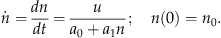
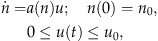
We consider a software system used by an organization at time 0 with initial number of features n ₀. The organization allocates an amount of enhancement effort u(t) at time t≥0 to write and add new features to the system. In practice, there is usually a limit on the total amount of effort that can be exerted at any given time. We therefore set an upper limit u ₀ on the effort u(t). Because new features cannot be installed and learnt by users instantly, we consider a time lag between the addition of a feature and the realization of its value, similar to that in Gaimon (1997). A continuous time function φ(t) is used to denote the lag‐of‐learning effect. As new features are added, new bugs are inadvertently introduced (Lanning and Khoshgoftaar 1995), and additional cost must be incurred to remove these bugs.

The values of n ₀, u(t), and T (lifetime of software) need to be chosen optimally to maximize the total discounted profit (benefit minus cost) over the lifetime of the released system. We will study a more complete model with software replacement in section 5, but for the single‐system model, this goal is achieved by balancing the benefits gained from adding new features with the cost of creating features, fixing bugs, and maintaining the system. In the rest of this section, we present expressions for the costs and benefits of feature addition and formulate the problem of optimally determining the enhancement effort.

3.1. Feature Growth

Let n(t) be the total number of features in the software system at time t. When adding a new feature, it is necessary to ensure that it is consistent with existing features (Mookerjee and Chiang 2002). Therefore, it becomes more difficult to add new features when there are more existing features, i.e., it is more difficult to enhance a complex system. This impact of complexity, called the Second Law of Program Evolution by Lehman (1980), has been considered in various studies (Kafura and Reddy 1987, Lehman and Ramil 2002).

As suggested by Ji et al. (2005) using the data collected from a NASA project (Heller et al. 1993), the amount of effort needed to add dn(t) features between time t and t+dt is u(t)dt, and is composed of: (i) a ₀·dn(t)—the direct feature creation effort and (ii) a ₁·dn(t)·n—the effort of integrating the newly created features with the existing n features. Here, a ₀ and a ₁ are positive constants. Hence, the rate of growth in the number of features can be modeled as the following non‐linear function of n:²,³ 1

As can be seen from Equation (1), for a system of size n, the higher the effort u, the faster new features can be added at time t. The denominator in the expression for represents the effect that as the system size n grows, the system becomes more complex and the effectiveness of enhancement effort decreases. Specifically, the constant a ₀ represents the effectiveness of feature creation effort and is inversely related to the enhancement productivity—a higher value of a ₀ leads to a slower growth in the number of features. On the other hand, the constant a ₁ (feature growth coefficient) captures the impact of connectivity in the system on the effort required to write new features. The connectivity affects feature growth because, as discussed earlier, the programmers need to ensure that the new features are consistent with the features that already exist in the system (Mookerjee and Chiang 2002).

3.2. Value Generation

New features usually take a certain amount of time for the users to learn and assimilate (Gaimon 1997). Therefore, for each new feature, we expect a gradual transition to the point in time when the feature begins to provide full value. Similar to Gaimon (1997), we incorporate a continuous time function φ(t) to represent the lag‐of‐learning effect in our model with .⁴ Therefore, the value per unit time generated in the system at time x by a feature released at time t (x>t) is modeled as 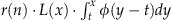. The term is the percentage of value of a feature released at t that has been learnt by time x. Factors r(n) and L are explained below.

The factor r(n) is the marginal value of each new feature added at time t. It is a decreasing function of the system size n: as the system grows larger, the marginal value of a new feature diminishes. This result has been supported by the empirical studies in Boehm (1981) (based on several software projects, mostly in the aerospace industry) and Little (2004) (based on the software used in the oil and gas industry). Therefore, we let r(n) be 2

Even though r(n) is a linear function of n, the value generated by the features is clearly a non‐linear function which is derived in the supporting information Appendix S1. It is consistent with the past empirical studies. As users gain experience with the system, they are better able to use it to extract benefit. This learning‐by‐doing impact on production‐cost reduction and productivity gain has been studied by Arrow (1962) and supported empirically by Schilling et al. (2003) based on an experimental design with 90 subjects. The factor L captures the learning‐by‐doing impact on the overall value of the system, and is an increasing non‐linear function of the duration for which the users have used the system. For our analysis in section 6, we use a concave increasing function for L based on the past empirical studies.

3.3. Cost of Fixing New Bugs

As mentioned earlier, adding new features often introduces new bugs into the system (Lanning and Khoshgoftaar 1995). We denote the cost of fixing bugs at time t by 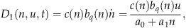3 which is consistent with the previous research on software defects (Ji et al. 2005).

We assume that the bugs introduced by the newly added features are fixed without delay. In (3), c(n) represents the impact of the number of features on the cost of fixing bugs. As the system becomes larger (more complex), more bugs are created when adding the same number of features (Lehman and Ramil 2001). This outcome is supported in an empirical study by Harter and Slaughter (2003), which was based on the monthly data collected over a decade from nine infrastructure activity centers in the systems integration division of a major information technology firm. Also, the empirical study by Banker et al. (1993), which was based on the data collected at a major regional bank with a large investment in the computer software, shows that it costs more to fix the same number of bugs in a complex system than it does in a simpler system. Accordingly, we specify 4 where c ₀ represents the constant part of the cost of fixing bugs when new features are added to the system. Factors such as programming quality and the criticality of functionality provided by a system affect c ₀. The coefficient c ₁ measures the (variable) system‐size effect on the cost of fixing bugs (Banker et al. 1993, Lehman and Ramil 2001).

As the developers design more features and become more familiar with the system, the development process becomes more reliable over time. Thus, as shown in the empirical study by Harter and Slaughter (2003), with an improvement in the development process, the defect rate, measured by the number of defects per KLOC (thousand line of code), decreases. Therefore, the factor b _q(n) in (3) is modeled as a decreasing function of the increase in system size from its initial size. It is a proxy for the experience gained through the amount of work done on the system, reflecting the effect of process maturity on software quality. Formally, we let 5 where is the limit for the impact of process improvement on the defect rate. Using the expressions for c(n) and b _q(n) (given by (4) and (5), respectively) in Equation (3), it is easy to see that the cost of fixing bugs D ₁(n, u, t) is a non‐linear function, which is consistent with the past empirical studies.

3.4. Maintenance Cost

A software system does not operate in isolation and may fail to provide the intended benefits due to any of the following reasons: (a) changes in the operating environment, (b) deterioration of the hardware platform, (c) changes in other software systems with which it interacts, (d) changes in business requirements, etc. Hence, the organizations need to incur maintenance costs during the lifetime of the system. The cost of maintaining a system typically increases as the system ages or becomes more complex (Kafura and Reddy 1987). This result has been supported by several empirical studies, e.g., Banker et al. (1993) (based on the data collected at a major regional bank) and Gibson and Senn (1989) (based on a 3 × 3 factorial design using experienced programmers). Hence, we model the cost of maintaining (we are, of course, referring here to corrective maintenance only) the system as 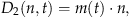6 where m(t) is an increasing non‐linear function of t. As a result, D ₂(n, t) is also the non‐linear function of t. For our analysis in section 6, we use an exponential function for m(t), as suggested by the past empirical studies.

3.5. Optimization Problem

The optimization problem consists of choosing the optimal system lifetime T, the optimal development effort u, and the optimal initial features n ₀, in order to maximize the total discounted profit gained from the system between [0, T]. 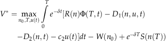Given that the cost of writing and adding new features to the system is c ₂ per unit effort, the optimal control problem with a continuous discount rate δ is the following (see supporting information Appendix S1) 5: 7 subject to where a(n)=1/(a ₀+a ₁ n). In this optimization problem, R(n)=(r ₀−r ₁ n/2)n is the system value generated at time t. It is a direct function of the number of features adjusted by the function Φ (see the expression for this function in the supporting information Appendix S1) that combines both the lag‐of‐learning and the learning‐by‐doing effects. Expressions of D ₁(n, u, t) and D ₂(n, t) are given in Equations (3) and (6), respectively. Finally, the function W(n ₀) represents the initial cost to obtain a system with number of features n ₀ (at time t=0) and e ^−δT S(n(T)) is the discounted salvage value of the system at the end of its useful life (i.e., at t=T).

As discussed earlier, a software system usually has a close‐down stage during its life‐cycle when the software is withdrawn (Rajlich and Bennett 2000). In our model, the lifetime T refers to the time of the close‐down stage. Moreover, organizations stop enhancing the system in the phase‐out stage (Rajlich and Bennett 2000). We obtain the optimal time of both the phase‐out and the close‐down stages, along with the optimal enhancement trajectory.

In section 4, we derive closed‐form expressions for optimal u and n ₀ as well as the optimal lifetime T for general forms of r(n), b _q(n), and m(t). In section 6, we will use specific forms of r(n), b _q(n), and m(t) for the purpose of numerical illustrations.

4. Optimal Solution

In this section, we first derive a closed‐form solution to the optimal control problem in (7). We next analyze the optimal effort under the following two scenarios: (a) the initial number of features n ₀ in a released system is smaller than a threshold value N (specified later) and (b) n ₀ is larger than N.

4.1. Solution Methodology

In order to solve the control problem, we start with the Hamiltonian (Sethi and Thompson 2000), which can be written as 8 where R _adj=R(n)Φ−D ₂ and λ ₁ is the adjoint variable corresponding to the state variable n that satisfies the following equation: 9

The adjoint variable λ ₁ can be interpreted as the change in the objective function for a small change in the corresponding variable n (Sethi and Thompson 2000). It can also be interpreted as the shadow price per feature. In other words, λ ₁ is the marginal value of adding new features to the system. Therefore, when the system is phased out at t=T, then λ ₁ equals the marginal salvage value. Also, the optimal solution should yield a positive λ ₁ whenever the development effort u is strictly positive. In the supporting information Appendix S3, we verify that it is indeed the case. Interestingly, the opposite is not true, i.e., a positive λ ₁ does not necessarily indicate a strictly positive u. The reason is that, as long as the marginal value of adding new features (i.e., λ ₁) is less than the marginal cost of the development effort (i.e., c ₂), it is not worthwhile adding new features (i.e., u=0), even though we might have a positive value for λ ₁.

We rewrite the Hamiltonian in (8) as 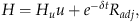10 where 11

From Equation (10), we can see that the Hamiltonian is linear in the control variable u. Therefore, we have the following solution form for an optimal control problem (7): 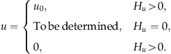12

A nice feature of the above solution form is that it has reduced a dynamic optimization problem (7) over the interval [0, T] to a sequence of static optimization problems (12), one for each instant t. That is, we only need to maximize the Hamiltonian at each instant t∈[0 T]. This result can be explained as follows. The first term on the right‐hand side of the Hamiltonian (8) is the direct value contribution to the objective function in (7). The second term is the indirect contribution of the new feature additions to the objective function since λ ₁ can be regarded as the marginal value of adding new software features to the system. If we were to maximize only the first term of the Hamiltonian at each point t, we would not maximize the objective function. We exert the maximum possible effort (i.e., u=u ₀) when H _u is positive and the minimum effort (u=0) when H _u is negative. Such a solution form is called bang‐bang. In the time period when H _u=0, the optimal level of the development effort u can be derived from the condition H _u=0. Such a control (i.e., the optimal choice for u) is called the singular control.

4.2. Closed‐Form Solution and Analysis

We first obtain a closed‐form solution for a given n ₀ and summarize the related results below.

Theorem 1. (For proof, see the supporting information Appendix S2). The general form of the optimal solution depends on the initial number of features n ₀ as follows:

(i)

When n ₀ is smaller than a given threshold value N, then

(a)

for 0≤t<T ₁, u=u ₀,

(b)

for T ₁≤t<T ₂, , and

(c)

for T ₂≤t≤T, u=0.

(ii)

When n ₀ is larger than the threshold value N, then

(a)

for , u=0,

(b)

for , , and

(c)

for T ₂≤t≤T, u=0.

The expressions for n, T ₁, , T ₂ , T, N, and g ₁ are given in the supporting information Appendices S2 and S3.

As shown in Theorem 1, the solution form can be categorized into two types according to the initial number of features in the released system. Figures 1 and 2 present the optimal trajectories of u and n for these two types of systems. If the initial number n ₀ is below a certain threshold value N, then maximum effort u=u ₀ is spent on adding new features from t=0 to reach a steady‐growth state (see Figure 1a). We refer to such a system as one exhibiting fast‐growth. In Figure 1b, the solid line between 0 and T ₁ denotes the feature growth curve for a given n ₀, which is below N. Note that, even though u=u ₀ between 0 and T ₁, n(t) is non‐linear because of the functional form of (see Equation (1) in section 3.1 and Equation (B.2) in the supporting information Appendix S2).

Figure 1

(a) Optimal Effort Allocation in Fast‐Growth System. (b) Optimal Feature Growth in Fast‐Growth System

Figure 2

(a) Optimal Effort Allocation in Slow‐Growth System. (b) Optimal Feature Growth in Slow‐Growth System

Next, the solid line between T ₁ and T ₂ represents the steady‐growth curve. The dotted line between 0 and T ₁ indicates that if n ₀ was equal to N, then the feature growth curve would have followed the steady path starting from t=0 rather than from t=T ₁. In other words, when n ₀=N, then T ₁=0. Also, note that T ₁=T ₂ is a special case where the singular control is not supported and the solution is pure bang‐bang. It is easy to check whether T ₁ =T ₂ by comparing the expressions of (C.6) and (C.7) in the supporting information Appendix S3.

Once the steady‐growth state is reached at T ₁, the development team spends an amount of development effort to balance the value of feature growth and the associated cost. As the system becomes more complex, the marginal cost of feature creation, bug fixing, and system maintenance eventually exceeds the value an additional new feature could bring. Thus development effort stops at T ₂. However, the system is still valuable until the maintenance cost surpasses the value of the system. The system life ends at T when the software is withdrawn. Note that the value of T ₂ in the solution is the optimal time for the phase‐out stage of the software life cycle, and the value of T is the optimal time for the close‐down stage (Rajlich and Bennett 2000).

The dotted line in Figure 2b between 0 and represents the steady‐growth curve, similar to that in Figure 1b. We would also like to point out that, in Figure 2, the larger the initial size n ₀, the longer the time before enhancement starts (i.e., ). Moreover, the result in the first phase of Figure 2 (i.e., when ) is opposite to general notion that the maximum effort should be spent in the initial time period. Hence, it is really important for the managers to compare the initial number of features in the released system with the threshold value N before making the decision regarding the enhancement effort.

Since we assume in the proof of Theorem 1 that H _u(t)<0 for T ₂<t≤T, we validate it numerically using the following functional forms: φ(t)=t ^α−1 e ^−t/β β ^−α/(α−1)!, L(t)=l ₀+l ₁·t ^1/2, , , and S(n)=s ₀ n. The details of parameters values used for this experiment are given in Table A1 of the supporting information. We present the rationale for using these functional forms and parameter values later in section 6.1. In order to validate the results for different problems instances, we vary the value of α from 1 to 10 in the increment of one. For each of these 10 problem instances, we find that H _u(t) is indeed negative for T ₂<t≤T.

To completely solve the maximization problem (7), we need to find the optimal value of n ₀. We could use a brute‐force search: since we could find the value of V for any given n ₀ using the results from Theorem 1, we vary n ₀ to maximize V. However, the weakness of such an unguided search algorithm is that it becomes harder to choose in which direction to change n ₀ (upwards or downwards) when we move close to the optimum point. We present a smarter algorithm using ideas from optimal control theory and present it in Corollary 1.

Corollary 1. The optimal satisfies the equation , where λ ₁ is given in the supporting information Appendix S3. For a given n ₀ , we should increase n ₀ if ; otherwise, we should decrease n ₀.

The intuition for Corollary 1 is the following. If the marginal value λ ₁(0) of adding a new feature at t=0 is higher than the corresponding marginal cost 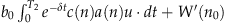, then we should add more features at the beginning by increasing n ₀. On the other hand, if λ ₁(0) is lower than the corresponding marginal cost, then we should decrease n ₀.

5. Software Replacement Cycle—Long‐Term View

In this section, we extend our model by considering that a new system is available in the market for adoption any time at or after T. Since the new system usually incorporates the superior technology (Chan et al. 1996, Sneed 1995), we consider that the new system performs the same functions equally well or better, but requires less maintenance effort. More specifically, we consider the marginal value of a feature in the new system as , where r(n) is the marginal value of the existing system defined in Equation (2). Also, the marginal cost of maintenance m ^new is less than the marginal maintenance cost m defined in Equation (6). However, in our model, it is easy to incorporate the higher maintenance effort for the new system.

The organization needs to spend effort in accumulating knowledge about the new system before its adoption. Let us denote this effort at time t by v(t) and the status of knowledge by K(t). The rate of growth in knowledge K depends on the effort of learning v and the remaining unknown knowledge (1−K). Hence 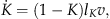13 where l _K is a factor that influences the growth of knowledge. Once the firm decides to adopt the new system, the existing features are implemented in the new system. Hence, the initial number of features in the new system is the same as the number of features in the old system at the time of adoption. This conversion cost has a fixed and a variable component. The variable cost decreases with the knowledge gained about the new system, but increases with system size. Hence, the conversion cost Z(n, K) is 14 where z ₁ is the fixed cost of conversion, z ₂ is the variable cost of conversion, and a _K is a factor that affects the impact of knowledge. In (14), ρ indicates that the variable cost may increase with the size of the system in a non‐linear fashion.

Let us redefine T to be the time when the second system is withdrawn and let T ₃ denote the time of adoption to the new system. The time T ₃ corresponds to time T in the previous single‐system model. The modified maximization problem can now be written as   15 subject to (1), (13), and 0≤u+v≤u ₀, where .

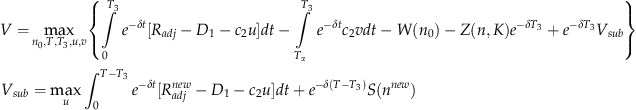
We can solve this model in two stages. In the first stage, we can easily solve the problem of enhancing the new system between T ₃ and T, for which the solution form is similar to the solution of the single‐system problem. In this section, we focus on the second stage where we solve the problem of enhancing the first system between 0 and T ₃.

As before, we can write the Hamiltonian as the following: 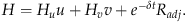16

The expressions for H _u and R _adj are the same as those in the previous model and H _v is defined in the supporting information Appendix S4. Since the Hamiltonian is bilinear in the control variables u and v, the Hamiltonian (16) can be optimized by a form for u described in (12) and a similar solution form for v. We depict the solution form by the timeline in Figure 3 ⁶ and summarize the results in Theorem 2.  Theorem 2.⁷ (For proof, see the supporting information Appendix S4). The optimal solutions for u and v are given as follows:

Figure 3

Timeline for the Solution Form in Software Replacement Model

(a)

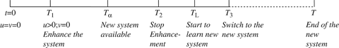
for 0≤t<T ₁, u=0 and v=0.

(b)

for T ₁≤t<T ₂, , and for T ₁≤t<T _L , v=0.

(c)

for T ₂≤t<T ₃ , u=0, and for T _L≤t≤T ₃ , v=u ₀.

(d)

for T ₃≤t≤T, the solutions can be obtained from Theorem 1 except that we replace m by m ^new, r ₀ by , and r ₁ by .

The expressions for T ₁ , T ₂ , T _L , and T are given in the supporting information Appendix S4. The expressions for n and g ₁ are the same as those in Theorem 1.

An interesting implication of Theorem 2 is that T ₂ is smaller than T _L, i.e., the “enhancement effort” in the first system stops before the learning of the new system starts. This result directly follows from the following two observations: (i) part (c) of Theorem 2 shows that v=u ₀ for T _L≤t≤T ₃, and therefore u=0 in this region (because 0≤u+v≤u ₀), and (ii) part (b) of the theorem shows that u>0 for T ₁≤t<T ₂.

6. Further Analysis and Managerial Insights

Using the closed‐form solutions developed in the previous sections, we present several numerical results and provide important managerial insights. We begin by presenting some specific functional forms and baseline values for the numerical analyses. In the subsequent sub‐sections, we study the impact of learning lag and examine the effects of different parameters on the optimal enhancement and upgrade strategies.

6.1. Functional Forms and Baseline Values

Thus far we have obtained analytical results without using any specific functional forms for φ(t), L(t), m(t), and W(n ₀). In order to gain further managerial insights, we consider following functional forms for φ(t), L(t), m(t), and W(n ₀).

Feature learning rate: φ(t)=t ^α−1 e ^−t/β β ^−α/(α−1)! (α and β are positive integers)

Similar to Gaimon (1997), we use a continuous gamma distribution (Korn and Korn 2000) to model gradual transition of learning to reach the full value of the feature. The parameter α represents the peak of the learning rate while β represents the duration in which learning is significant. By changing α and β, we can examine the effect of learning lag on the optimal policy.

Learning‐by‐doing effect: L(t)=l ₀+l ₁·t ^1/2

As users interact and gain experience with the system, it becomes more valuable for them. The benefit of learning‐by‐doing is commonly found to exhibit diminishing returns (Arrow 1962, Schilling et al. 2003). Hence, we use a concave increasing function of t for L(t).

Maintenance cost rate

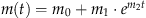
The cost of maintaining the system increases as the system ages (Gibson and Senn 1989, Kafura and Reddy 1987). Therefore, we model m(t) as an increasing function of time t.

Initial system cost with size n ₀:

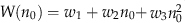
To develop or purchase a system with size n ₀, there is a fixed cost (w ₁) and a variable cost (w ₂ n ₀) that is proportional to the initial size n ₀. After the system is obtained, it needs to be implemented by the organization. The cost of implementation depends on the complexity of the system and is usually higher than the purchase cost (Austin et al. 2003). Hence, we use to represent the cost of the implementation as a convex function of the system size.

System salvage value S(n): S(n)=s ₀ n

We let S(n) be proportional to the final system size n that directly creates value.

We next present some numerical results and provide managerial insights using the baseline parameter values given in Table A1 of the supporting information. All the parameter values except r ₀ are the same for the existing and the new systems. When the new system is adopted, the time arguments in φ(t), L(t), and m(t) are reset to 0 to denote a new learning and maintenance cycle.

As the quality of development process improves, the bug rate decreases with b ₀=2.5 × 10⁻⁴ and , in line with the empirical findings of Harter and Slaughter (2003). The cost parameters c ₀ and c ₁ are chosen such that each bug costs about US$1000 to remove. For a system of size about 500, the initial maintenance cost rate is about US$1000/week and the initial gross revenue rate is US$100,000/week; the maintenance cost rate increases exponentially with time while the revenue rate increases at a slower rate. We choose the values of w ₁, w ₂, and w ₃ such that all three terms of the initial system cost are comparable. It takes about 2 weeks (α=2) to reach the peak of learning rate after each new feature is released and on average 1 month (αβ=4) to learn the new feature. It takes about 1 year (50 weeks) for the system to double in value due to the learning‐by‐doing effect (l ₀+l ₁·50^1/2≈2). Other parameter values are chosen to be representative of real‐world systems.

6.2. Impact of Learning Lag

In this section, we analyze the results of the first model (which is presented in section 4). Here, we study the impact of learning lag on (i) the optimal value of the initial number of features, (ii) the net enhancement value, (iii) the amount of improvement from using the optimal solution as compared with the solutions from two base policies, and (iv) the regions for maximum‐growth, steady‐growth, and no‐growth. This study will help managers in identifying the region where the optimal policy is most beneficial, which in turn would facilitate comparison studies based on the administrative burden involved in implementing the optimal policy. This analysis also sheds light on the interaction between the initial number of features in the software and the amount of net enhancement that is optimally needed after its adoption.

In Figure 4a, the initial number of features n ₀ and the number of new features added (n(T ₂)−n ₀) are plotted as a function of the learning‐lag parameter α: the higher the value of α, the slower the learning of a new feature with the average time of learning a new feature being α·β and variance α·β ². Figure 4a shows that as α increases, n ₀ increases and the amount of net enhancement decreases. The explanation is as follows: When a system takes more time to learn, it is better to squeeze more features into the initial system and generate the value earlier rather than adding more features later. However, the final size of the system n(T ₂) decreases with an increase in α. This is confirmed by adding the ordinates of two curves in Figure 4a.

Figure 4

(a) Impact of Learning Lag (α) on Initial Number of Features (n ₀) and Added New Features. (b) Impact of Learning Lag (α) on Enhancement Policies

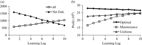
In order to study when the optimal policy is most beneficial, we compare it with two base policies: (a) maintenance‐only policy and (b) uniform‐allocation policy. As discussed earlier, in the maintenance‐only policy, only exogenous requests trigger maintenance effort. In this policy, no enhancement effort is allocated for adding more features. Hence, the number of features stays the same throughout the system lifetime. For the comparison purpose, this number is chosen to be n(T ₂) of the optimal policy. Therefore, the profit is given by 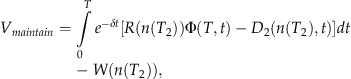with T ₂ and T being the same as those of the optimal policy.

In the uniform‐allocation policy, a constant level of enhancement effort is spent from time 0 to T to enhance the system with the initial size being n ₀ and the final size n(T ₂). As in the maintenance‐only policy, values of n ₀, T, and n(T ₂) are given by the optimal policy, and u _uniform can be solved similarly as . Therefore, the profit is given by

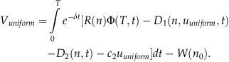
Similarly, the profit under the optimal policy is obtained by replacing u _uniform in the above expression with the optimal enhancement effort determined from (15).

Figure 4b plots the profit values as a function of the learning lag α. As we can see in this figure, the optimal policy outperforms both the maintenance policy and the uniform‐allocation policy significantly in the low α region. However, the benefit of the optimal policy diminishes as α increases. This phenomenon can be explained by the results of Figure 4a. As shown in Figure 4a, the amount of net enhancement decreases with an increase in α. One of the key aspects of the optimal policy is to allocate the enhancement effort optimally, and therefore it is less valuable if there is less enhancement work needed.

We also study the impact of β on the performance of optimal policy and find similar results: an increase in β causes an increase in n ₀ and decrease in the net enhancement value. As a result, the performance of the optimal policy worsens with an increase in β and starts to converge with the other two policies. The details of this study are omitted for brevity.

Next, we extend this study to analyze the impact of α on three regions depicted in Figure 1: (a) maximum‐growth region (from time 0 to T ₁), (b) steady‐growth region (from time T ₁ to T ₂), and (c) no‐growth region (from time T ₂ to T). For each region, we examine the values of both the time duration and the net enhancement value. The results are presented in Table 1. For clarity, we also present the values of n ₀ in this table, which are the same as those in Figure 4a.

Table 1

Impact of the Learning Lag on Three Regions of Software Life‐Cycle

α	n ₀	Maximum‐growth region		Steady‐growth region		No‐growth region
α	n ₀	Duration	Net enhancement	Duration	Net enhancement	Duration	Net enhancement
1	580	13	843	71	761	175	0
3	680	10	690	66	714	185	0
5	780	8	536	60	664	197	0
7	880	6	382	55	618	205	0
9	1000	3	185	53	597	212	0

Table 1 shows that both the time duration and the net enhancement values decrease very sharply in the maximum‐growth region with an increase in α, whereas the reduction is much less steep in the steady‐growth region. This result is consistent with Theorem 1: an increase in α increases the initial number of features n ₀, bringing it closer to the threshold value N. When n ₀ is closer to N, the maximum amount of effort (u=u ₀) is needed for a smaller duration in order to reach the steady state, and therefore the time duration and the net enhancement decrease in the maximum‐growth region.

A related result is also presented in Table 1: the duration of the no‐growth period increases with an increase in α. This result can be attributed to the fact that when it takes longer to learn the features, it is more advantageous to use the system for a longer period after all the features have been created. Adding the time durations in three regions shows that the lifetime of the software also increases with an increase in α, albeit at a very slow rate, indicating that it is beneficial to keep the software longer when learning is slower.

The above study can help managers in understanding the impact of learning lag on the dynamics of feature enhancement, as well as in quantifying the effect of learning on the different stages of the software life cycle (such as the phase‐out stage and the close‐out stage). Now, in the next section, we analyze the results of the second model in order to gain interesting managerial insights regarding the software replacement decision.

6.3. Optimal Enhancement and Upgrade Strategy

Here we study the impacts of T (the time at which the new system is available for adoption), r ^new (the value of the new system), and the bug‐fixing cost on the optimal enhancement and upgrade strategies. For the first system, there are two possible enhancement strategies (E, NE): strategy E denotes that some enhancement is done on the first system after its adoption while strategy NE denotes that no enhancement is done on the first system. We classify the strategies of migrating to the new system into A and W. The strategy A denotes: “start learning the new system as soon it becomes available, and migrate immediately after learning it sufficiently.” Hence, for strategy A, T _L=T in Figure 3. On the other hand, the strategy W denotes: “when the new system becomes available, wait for some time before starting to learn the system.” Therefore, T _L>T in Figure 3 for strategy W.

In Figure 5, we examine the impact of on strategies by varying its value between 180 and 300. Also, we change the values of both c ₀ and c ₁ simultaneously such that the ratio for each of them from its corresponding baseline value varies between 0 and 2. Here, the higher values of c ₀ and c ₁ lead to a higher cost of fixing bugs that are injected during enhancement. As shown in Figure 5, the optimal enhancement and migration strategies are divided into four regions depending on the value of the new system and the bug‐fixing cost:

Figure 5

Regions for Optimal Enhancement and Upgrade Strategies

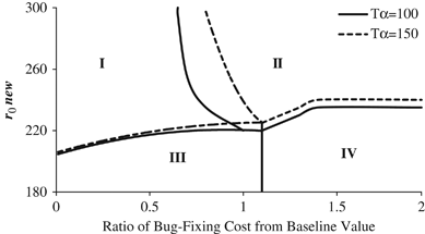
Region I: (E, A): It is better to enhance the initial system when the enhancement cost is low and plan an early migration when the new system has relatively high value.

Region II: (NE, A): It is better to do no enhancement on the initial system since the enhancement cost is high and plan an early migration since the value of the new system is relatively high.

Region III: (E, W): Enhance the initial system since the enhancement cost is low and plan a late migration since the value of the new system is relatively low.

Region IV: (NE, W): Do no enhancement on the initial system since the enhancement cost is high and plan a late migration to the new system that has relatively low value.

As the second system appears earlier, i.e., T becomes smaller, Region II expands to the left and downward. That is, it becomes more attractive to do no enhancement on the first system (i.e., the NE strategy) and migrate to the new system as soon as possible (i.e., strategy A) since the new system can be used earlier and longer. As the second system appears earlier, Region III shrinks downward. That is, it is worthwhile to migrate earlier even if enhancing the initial system is the optimal strategy.

From Figure 5, we can see that the boundary between Region I and Region II is the most sensitive to the value of T. On the other hand, the boundary between Region III and Region IV remains roughly the same and is the least sensitive to the value of T since the optimal migration strategy in these two regions is to wait for some duration after the new system appears. Overall, when the new system is highly valuable compared with the existing system and the enhancement cost is moderate, the time of the availability of the new system has a strong impact on the enhancement strategy. Hence, in this region, improving the accuracy of estimating T is important.

We further study the effect of on the optimal policy by setting the bug‐fixing cost at its baseline value. In Table 2, we present the optimal values of the overall profit, the initial number of features in the first system (n ₀), the amount of net enhancements in the first system (Net Enh.1), and the amount of net enhancements in the second system (Net Enh.2), for different values of .

Table 2

Effect of the Value of New System

	Overall profit (10⁶)	n ₀	Net Enh.1	Net Enh.2
Region III
180	55.1	610	1534	0
220	65.2	110	2442	0
Region I
230	68.8	11	2594	0
235	71.1	0	2611	0
Region II
240	73.6	1075	0	2537
300	113.3	1140	0	3415

As can be seen from Table 2 (and from Figure 5), when increases, the optimal policy traverses Region III, Region I, and then Region II. As expected, the overall profit increases when the new system becomes more valuable. Moreover, the number of initial features in the first system decreases with an increase in within the first two regions where the optimal policy calls for enhancement on the first system. However, in these two regions, the amount of net enhancement to the first system (Net Enh.1) increases as increases while the amount of net enhancement to the second system (Net Enh.2) stays at 0. On the other hand, as increases further and traverses to Region II, it becomes optimal to have a higher value of n ₀ and make more enhancements to the second system with an increase in . As a result, the enhancement to the first system is 0.

The above result is very important for the managers because it shows that there is a threshold value of beyond which the optimal strategy reverses (for both the first system and the second system). Hence, it is strongly recommended for them to spend effort in estimating the value of accurately so that they can formulate the correct strategy.

Next, we study the effect of bug‐fixing cost on the optimal policy. The results are presented in Table 3. In Table 3, we change the values of both c ₀ and c ₁ simultaneously such that the ratio from the corresponding baseline value varies between 0.01 and 1.5 (the actual values of the ratio are given in the first column of the table).

Table 3

Effect of the Bug‐Fixing Cost

Bug‐fixing cost	Overall profit (10⁶)	n ₀	Net Enh.1	Net Enh.2
Region I
0.01	120.6	150	3047	562
Region III
0.2	107.0	180	2915	312
0.6	83.2	145	2703	0
1.0	62.2	195	2311	0
Region IV
1.3	58.1	1569	0	279
1.5	57.0	1608	0	0

As bugs become more expensive to fix, it becomes less attractive to add new features to the system. As a result, the enhancement amounts for both the first system (Net Enh.1) and the second system (Net Enh.2) decrease with an increase in the bug‐fixing cost. In Regions I and III, where the enhancements on the first system are substantial, the number of initial features n ₀ stays very small. When the bug‐fixing cost increases further and enters into Region IV, it is not viable to enhance the first system, i.e., Net Enh.1 is 0. In this case, it is better to have more features initially and less or no enhancement later on.

7. Conclusions and Future Research Directions

In this paper, we consider the problem of optimizing the initial number of features in a software system and the enhancement effort after it is adopted. As businesses rely more on software systems for their operational, tactical, and strategic decisions, it has become critical to enhance these systems continuously. However, enhancement also introduces new bugs in the systems. Therefore, it is important for an organization to optimize the effort to increase the number of features in its existing software system such that the system's net benefit is maximized. Moreover, as the features need to be added continuously, the optimal effort policy should be dynamic in nature. We must also consider the fact that there often exists a time lag between the appearance of a new feature and its full value being realized by users.

In solving the optimization problem, we jointly optimize the initial number of features, the enhancement effort over the system life cycle, and the time at which the software system should be withdrawn. We obtain optimal trajectories for the enhancement effort and the system growth. Using solutions characterized in closed‐form, we study the impact of several important parameters on the optimal number of initial features, the optimal enhancement effort trajectory, and the optimal duration to use a system before it must be withdrawn.

We find that when the initial number of features in a released system is below a threshold, then the maximum amount of effort should be exerted initially until the steady‐growth state for the system is reached. On the other hand, if the initial number of features in a system is above that threshold, no effort should be used to enhance the system immediately after its release, because the value of adding a feature at that time is less than the cost.

Further, we optimize the initial number of features and investigate the impact of learning lag on (i) the initial number of features, (ii) the net enhancement value, (iii) the amount of improvement from using the optimal solution as compared with the solutions from two base policies, and (iv) the regions for maximum‐growth, steady‐growth, and no‐growth. As the learning lag increases, the initial number of features increases and the amount of net enhancement decreases. As the strength of optimal solution lies in optimizing the enhancement effort, the improvement from using the optimal solution diminishes with an increase in the learning lag. Also, with an increase in learning lag, the time regime expands for no‐growth and shrinks for both maximum‐growth and steady‐growth. Hence, the total time for enhancement also reduces with an increase in learning lag.

Finally, we extend our model to consider the scenario where a new system is available for adoption while the existing system is being used. In this model, we optimize the enhancement and upgrade decisions simultaneously. Our analyses show that the timing of the availability of new system T has a high impact on the enhancement strategy when the new system is highly valuable compared with the existing system and the enhancement cost is moderate. Hence, it is recommended to spend more effort in improving the accuracy of estimating T in this region. Our results also show that it is important to estimate the value of the new system accurately because the optimal strategy reverses when the value of the new system exceeds beyond a given threshold.

There is an interesting extension possible to our model. In an open‐source environment, it has been observed that the functionalities in the Linux kernel exhibit a hyper‐linear growth rate (Robles et al. 2005). At first glance, this seems to contradict our assumption that adding features to a larger system is more difficult, leading to a decrease in the growth rate, ceteris paribus. However, the apparent contradiction arises from differences between the two development modes. In an open‐source environment, many tasks are performed outside the group of core developers, whereas in an in‐house development environment, most tasks are completed by the same development team. As pointed out by Robles et al. (2005), “the flexible and auto‐organized management of human resources usually found in those projects could be the reason of a growth rate higher than the one found in other, more rigid and planned cases.” It would be interesting to see how one can utilize the open‐source environment to enhance a system optimally.

Footnotes

Acknowledgments

We would like to express our gratitude to the Department Editor Cheryl Gaimon, the Senior Editor, and the two anonymous reviewers for their constructive comments. This paper has benefited greatly from their careful reading and insights.

¹ http://www.simplifythis.com

²For notational convenience, hereafter, we typically suppress the time notation (t) in state variables, control variables, and adjoint variables when no confusion arises. It is consistent with the notation used in most optimal control theory literature.

³Here, the feature growth rate is a linear function of u, which is consistent with the past studies such as . Considering a non‐linear function of u will make the model more general but add further complexity to the model and make it intractable. We admit that this linear assumption is a limitation of the model.

⁴Note that one can always choose a functional form of φ(t), where the full value of a feature can be realized in a finite time. Hence, presents the generalized scenario.

⁵From , we have (r ₀−r ₁ n)≥0. It imposes the following constraint on n: n≤(r ₀/r ₁). However, we do not need to consider this constraint explicitly because it is always satisfied in the optimal solution, as can be easily verified.

⁶Here, we focus on one scenario where the organization initiates enhancement only after it has used the existing (or new) system for a while and the new system appears in the market after the organization begins to enhance the existing system. Similarly, we solve other possible scenarios and compare the results in .

⁷For brevity, we only present the results for the case n ₀≥N in this theorem. However, similar to Theorem 1, it is easy to present the result for the other case, i.e., n ₀<N. For numerical studies in , we consider both cases.

References

Arrow

K. J.

1962. The economic implications of learning by doing. Rev. Econ. Stud. 29 (3): 155–173.

Austin

R. D.

Cotteleer

M. J.

Escalle

C. X.

. 2003. Enterprise Resource Planning. Harvard Business School Note 9‐699‐020.

Bala

Carr

. 2009. Pricing software upgrades: The role of product improvement and user costs. Prod. Oper. Manag. 18 (5): 560–580.

Banker

R. D.

Datar

S. M.

Kemerer

C. F.

. 1991. A model to evaluate variables impacting the productivity of software maintenance projects. Manage. Sci. 37 (1): 1–18.

Banker

R. D.

Datar

S. M.

Kemerer

C. F.

Zweig

. 1993. Software complexity and maintenance costs. Commun. ACM 36 (11): 81–94.

Banker

R. D.

Slaughter

S. A.

. 1997. A field study of scale economies in software maintenance. Manage. Sci. 43 (12): 1709–1725.

Banker

R. D.

Slaughter

S. A.

. 2000. The moderating effects of structure on volatility and complexity in software enhancement. Inf. Syst. Res. 11 (3): 219–240.

Bennett

Rajlich

. 2000. Software maintenance and evolution: A roadmap. Finkelstein

ed. Proceedings of Conference on the Future of Software Engineering. ACM, Limerick, Ireland, 73–87.

Bensoussan

Sethi

S. P.

. 2007. The machine maintenance and sale age model of Kamien and Schwartz revisited. Manage. Sci. 53 (12): 1964–1976.

10.

Boehm

B. W.

1981. Software Engineering Economics. Prentice Hall, Upper Saddle River, NJ.

11.

Boothroyd

Dewhurst

Knight

W. A.

2002. Product Design for Manufacture and Assembly. Marcel Dekker Inc, New York.

12.

Burch

Kung

. 1997. Modeling software maintenance requests: A case study. Cimitile

A. V.

Rajlich eds. Proceedings of 13th International Conference on Software Maintenance. IEEE, Bari, Italy, 40–47.

13.

Carrillo

J. E.

Gaimon

. 2000. Improving manufacturing performance through process change and knowledge creation. Manage. Sci. 46 (2): 265–288.

14.

Chan

Chung

S. L.

T. H.

. 1996. An economic model to estimate software rewriting and replacement times. IEEE Trans. Softw. Eng. 22 (8): 580–598.

15.

Chiang

I. R.

Mookerjee

V. S.

. 2004. A fault threshold policy to manage software development projects. Inf. Syst. Res. 15 (1): 3–19.

16.

Couger

J. D.

Colter

M. A.

. 1985. Maintenance Programming: Improved Productivity Through Motivation. Prentice‐Hall, Englewood Cliffs, NJ.

17.

Cusumano

M. A.

Selby

R. W.

. 1997. How Microsoft builds software. Commun. ACM 40 (6): 53–61.

18.

Dawande

Johar

Kumar

Mookerjee

V. S.

. 2008a. A comparison of pair versus solo programming under different objectives: An analytical approach. Inf. Syst. Res. 19 (1): 71–92.

19.

Dawande

Kumar

Mookerjee

V. S.

Sriskandarajah

. 2008b. Maximum commonality problems: Applications and analysis. Manage. Sci. 54 (1): 194–207.

20.

Dohi

Nishio

Osaki

. 1999. Optimal software release scheduling based on artificial neural networks. Ann. Softw. Eng. 8: 167–185.

21.

Eastwood

1993. Firm fires shots at legacy systems. Comput. Can. 19 (2): 17.

22.

Feng

Mookerjee

V. S.

Sethi

S. P.

. 2006. Optimal policies for the sizing and timing of software maintenance projects. Eur. J. Oper. Res. 173 (3): 1047–1066.

23.

Gaimon

1997. Planning information technology‐knowledge worker systems. Manage. Sci. 43 (9): 1308–1328.

24.

Gaimon

Napoleon

Ozkan

. 2009. Investments in Workforce Knowledge and Technological Capabilities. Working paper, Georgia Institute of Technology, Atlanta, Georgia.

25.

Gaimon

Thompson

G. L.

. 1984. Optimal preventive and repair maintenance of a machine subject to failure. Optim. Control Appl. Methods 5 (1): 57–67.

26.

Gibson

V. R.

Senn

J. A.

. 1989. System structure and software maintenance performance. Commun. ACM 32: 347–358.

27.

A. Y.

Porteus

E. L.

. 1995. Optimal timing of reviews in concurrent design for manufacturability. Manage. Sci. 41 (9): 1431–1447.

28.

Harter

D. E.

Slaughter

S. A.

. 2003. Quality improvement and infrastructure activity costs in software development: A longitudinal analysis. Manage. Sci. 49 (6): 784–800.

29.

Heineman

G. T.

Councill

W. T.

. 2001. Component Based Software Engineering: Putting the Pieces Together. Addison‐Wesley, Boston, MA.

30.

Heller

Valett

Wild

. 1993. Data Collection Procedures for the Software Engineering Laboratory (SEL) Database. Software Engineering Laboratory, NASA/Goddard Space Flight Center, Greenbelt, MD.

31.

Hou

Kuo

Chang

. 1997. Optimal release times for software systems with scheduled delivery time based on the HGDM. IEEE Trans. Comput. 46 (2): 216–221.

32.

Mookerjee

V. S.

Sethi

S. P.

. 2005. Optimal software development: A control theoretic approach. Inf. Syst. Res. 16 (3): 292–306.

33.

Jiang

Sarkar

. 2003. Optimal software release time with patching considered. Proceedings of 13th Annual Workshop on Information Technologies and Systems, Seattle, December 13–14, pp. 61–66.

34.

Kafura

Reddy

G. R.

. 1987. The use of software complexity metrics in software maintenance. IEEE Trans. Softw. Eng. SE‐13 (3): 335–343.

35.

Kamien

M. I.

Schwartz

N. L.

. 1971. Optimal maintenance and sale age for a machine subject to failure. Manage. Sci. 17 (8): B‐495–B‐504.

36.

Koch

H. S.

Kubat

. 1983. Optimal release time of computer software. IEEE Trans. Softw. Eng. SE‐9: 323–327.

37.

Korn

G. A.

Korn

T. M.

. 2000. Mathematical Handbook for Scientists and Engineers. Dover Publications Inc, Mineola, NY.

38.

Koushik

M. V.

Mookerjee

V. S.

. 1995. Modeling coordination in software construction: An analytical approach. Inf. Syst. Res. 6 (3): 220–254.

39.

Kulkarni

V. G.

Kumar

Mookerjee

V. S.

Sethi

S. P.

. 2009. Optimal allocation of effort to software maintenance: A queuing theory approach. Prod. Oper. Manag. 18 (5): 506–515.

40.

Lanning

D. L.

Khoshgoftaar

T. M.

. 1995. The impact of software enhancement on software reliability. IEEE Trans. Reliab. 44 (4): 677–682.

41.

Lehman

M. M.

1980. Programs, life cycles, and laws of software evolution. Proc. IEEE 68 (9): 1060–1076.

42.

Lehman

M. M.

Ramil

J. F.

. 2001. Rules and tools for software evolution planning and management. Ann. Softw. Eng. 11 (1): 15–44.

43.

Lehman

M. M.

Ramil

J. F.

. 2002. Software evolution and software evolution processes. Ann. Softw. Eng. 14 (1): 275–309.

44.

Lientz

B. P.

Swanson

E. B.

Tompkins

G. E.

. 1978. Characteristics of application software maintenance. Commun. ACM 21 (6): 466–471.

45.

Little

2004. Value creation and capture: A model of the software development process. IEEE Softw. 21 (3): 48–53.

46.

Liu

Dawande

Mookerjee

V. S.

. 2007. Value‐driven creation of functionality in software projects: Optimal sequencing and reuse. Prod. Oper. Manag. 16 (3): 381–399.

47.

McConnell

1997. Annualized software delivery. IEEE Softw. 14 (1): 103–104.

48.

Mookerjee

V. S.

Chiang

I. R.

. 2002. A dynamic coordination policy for software system construction. IEEE Trans. Softw. Eng. 28 (7): 684–694.

49.

Okumoto

Goel

A. L.

. 1980. Optimum release time for software systems based on reliability and cost criteria. J. Syst. Softw. 1: 315–318.

50.

Rahmandad

2005. Dynamics of platform‐based product development. Sterman

J. D.

Repenning

N. P.

Langer

R. S.

Rowe

J. I.

Yanni

J. M.

, eds. Proceedings of 23rd International Conference on System Dynamics Society. The System Dynamics Society, Boston, MA.

51.

Rajlich

V. T.

Bennett

K. H.

. 2000. A staged model for the software life cycle. IEEE Comput. 33 (7): 66–71.

52.

Robles

Amor

J. J.

Gonzalez‐Barahona

J. M.

Herraiz

. 2005. Evolution and growth in large libre software projects. Proceedings of Eighth International Workshop on Principles of Software Evolution, Lisbon, Portugal, pp. 165–174.

53.

Schilling

M. A.

Vidal

Ployhart

R. E.

Marangoni

. 2003. Learning by doing something else: Variation, relatedness, and the learning curve. Manage. Sci. 49 (1): 39–56.

54.

Sethi

S. P.

Thompson

. 2000. Optimal Control Theory: Applications to Management Science and Economics. Kluwer Academic Publishers, Boston, MA.

55.

SimplifyThis.

2008. Update: Menu Replaced by Buttons. Available athttp://www.simplifythis.com/blog/?cat=3(accessed date October 27, 2010).

56.

Sneed

H. M.

1995. Planning the reengineering of legacy systems. IEEE Softw. 12 (1): 24–34.

57.

Sutherland

1995. Business objects in corporate information systems. ACM Comput. Surv. 27 (2): 274–276.

58.

Swanson

E. B.

1976. The dimension of maintenance. Yeh

R. T.

Ramamoorthy

C. V.

, eds. Proceedings of 2nd International Conference on Software Engineering. IEEE, San Francisco, CA, 492–497.

59.

Swanson

E. B.

Beath

C. M.

. 1989. Reconstructing the systems development organization. MIS Q. 13 (3): 293–307.

60.

Tan

Mookerjee

V. S.

. 2005. Comparing uniform and flexible policies for software maintenance and replacement. IEEE Trans. Softw. Eng. 31 (3): 238–255.

61.

Thompson

G. L.

1968. Optimal maintenance policy and sale date of a machine. Manage. Sci. 14 (9): 543–550.

62.

Whittaker

1999. What went wrong? Unsuccessful information technology projects. Inf. Manage. Comput. Secur. 7 (1): 23–30.

63.

Wilcox

2002a. Judge orders Microsoft to reveal code. CNET News, February 16. Available athttp://news.com.com/2100‐1001‐839356.html(accessed date August 11, 2010).

64.

Wilcox

2002b. RealNetworks reveals code in single helix. CNET News, October 29. Available athttp://news.com.com/2100‐1023‐963704.html(accessed date August 11, 2010).

65.

Zhang

Tsai

J. J. P.

. 2005. Machine Learning Applications in Software Engineering. World Scientific Publishing Company Incorporated, Singapore.