Competitive and Collaborative Quality and Warranty Management in Supply Chains

Abstract

Product quality and product warranty coverage are two important and closely related operational decisions. A longer warranty protection period can boost sales, but it may also result in dramatically increased warranty cost, if product quality is poor. To investigate how these two decisions interact with each other and influence supply chain performance, we develop a single‐period model with a supplier that provides a product to an original equipment manufacturer, which in turn sells it to customers. Customer demand is random and affected by the length of the product warranty period. Warranty costs are incurred by both the supplier and the manufacturer. We analyze two different scenarios based on which party sets the warranty period: manufacturer warranty and supplier warranty. Product quality is controlled by the supplier, and the manufacturer determines the ordering quantity. We analyze these decentralized systems and provide the structural properties of the equilibrium strategies. We also compare the results of centralized and decentralized systems and identify the conditions under which one system provides a longer warranty and better product quality than the other. Our numerical study further shows that, in decentralized settings, when the warranty period is determined by the firm sharing the larger proportion of total warranty costs, the supply chain can achieve greater system‐wide profit. Both parties can therefore benefit from properly delegating the warranty decision and sharing the resulting additional profit. We further design a supplier‐development and buy‐back contract for coordinating decentralized supply chains. Several extensions are also discussed.

Keywords

product quality warranty period warranty‐dependent demand Nash equilibrium supply chain coordination

1. Introduction

In today's highly competitive marketplace, product quality is increasingly important to the success of manufacturing firms. Although all consumers prefer high‐quality products, they are often unable to assess product quality directly. Instead, they consider a product's warranty coverage to be a signal of quality, often perceiving a longer coverage period to be an indicator of better quality and a better service level (Boulding and Kirmani 1993,Purohit and Srivastava 2001).¹ Hence, many companies, particularly those in the automobile and consumer‐electronics industries, often use warranty policy as a marketing strategy to attract customers, thereby stimulating demand. A warranty is most commonly an agreement with customers to repair or replace a purchased product in the case of failure. Although a longer warranty protection period may boost sales, it can also result in dramatically increased warranty cost, if the product is of poor quality. Thus, the offering of a long warranty period often results in a significant financial burden for companies that lack an integrated product quality control and warranty policy. For example, in 2000, the Big Three automakers' annual warranty costs were around US$6 billion, or an average of US$500 per unit, in North America (Allen 2001). Coordination of the quality control and warranty strategy is therefore critical to supply chain performance.

We develop a supply chain model with one supplier and one manufacturer, where the manufacturer is an original equipment manufacturer (OEM) that purchases parts or final products from a supplier and sells them to customers. The products are covered by a warranty policy. Customer demand is random and depends on the length of the warranty period. The supplier determines product quality and the manufacturer determines the ordering quantity. The warranty policy can be determined by either the supplier or the manufacturer. Both OEM and supplier warranties can be found in, for example, the PC hard disk market. Some PC OEMs may purchase hard disks from suppliers without a warranty and then set a warranty for the entire PC themselves when selling to consumers. Hence, the hard disk is covered only by the OEM warranty. Others, however, may purchase hard disks with warranty coverage from the supplier. In the latter scenario, although the OEM still provides a warranty for the entire PC, the warranty period is shorter (commonly 1–2 years) than the supplier warranty on the hard disk (commonly 3–4 years). Thus, the hard disk can be considered to have only a supplier warranty. This phenomenon is also observed in the market for other PC components, such as optical drives, memory chips, video cards, and even CPUs ( The PC Guide 2008). Both the supplier and the manufacturer incur warranty costs that depend on product quality and the length of the warranty period, and the objective of both is to maximize their own expected profit.

Warranty cost is certainly a critical issue when a firm determines its warranty policy. When an item under warranty is returned for corrective actions, a warranty cost will be incurred in the form of material costs, labor/repair costs, and managerial costs. These costs are usually shared by the different parties in the supply chain, as supply chains are increasingly integrated today. For instance, an OEM often needs to process customer claims initially, thereby incurring handling and managerial costs. In most cases, it will then send the failed units back to its supplier for repairs, thus resulting in repair costs for the supplier. The warranty cost depends on both the length of the warranty period and product quality. The longer the warranty period and/or the poorer the product quality, the higher the potential warranty cost. However, due to relentless price squeezing from powerful buyers, profit‐starved suppliers are often forced to cut expenditures in such key areas as quality management systems in an effort to reduce costs, which can lead to a serious deterioration in product quality and, in turn, increased warranty costs for the supply chain. It is thus important to analyze the interaction between quality‐improvement and warranty policies and their impact on supply chain performance. Moreover, a more powerful firm may wish to decide the warranty policy itself and force the other party to bear more of the warranty cost without really knowing the consequences for supply chain performance. These issues give rise to the following research questions. In what circumstances is the entire supply chain better off if the upstream supplier, or downstream manufacturer, sets the warranty policy? Which warranty scenario leads to better product quality or a longer warranty period? What type of contract can coordinate the decentralized warranty, quality, and ordering decisions and allow supply chain profit to be divided freely?

To answer these questions, we examine two situations in our model, in which either the manufacturer or the supplier determines the warranty protection period. The first is referred to as the manufacturer warranty: the supplier and the manufacturer first determine the product quality and the warranty, respectively, and the ordering decision is then taken by the manufacturer. We show that the quality–warranty game has a unique pure‐strategy Nash equilibrium. The equilibrium warranty period decreases and product quality deteriorates when the manufacturer shares more of the warranty costs. The second is referred to as the supplier warranty: the supplier sets both the warranty period and the product quality level before the manufacturer makes an order. We analyze and solve this situation as a Stackelberg game. In neither scenario does the supplier's expected profit increase with the wholesale price. Moreover, under a supplier warranty, the manufacturer may not be better off with a lower wholesale price. These results imply that it is not always beneficial for a supply chain partner to squeeze the other party's margins in such a supply chain. The results of the two decentralized scenarios are then compared. When the firm with the higher marginal revenues with respect to the warranty and a smaller proportion of the total warranty costs sets the warranty, the supply chain sells better quality products with a longer warranty.

Our numerical results also show that the supply chain's choice of a supplier warranty or a manufacturer warranty depends on how the warranty costs are shared between the two firms. The supplier (manufacturer) warranty is usually better for the system when the supplier (manufacturer) shares a larger proportion of the supply chain warranty costs. We further design a supplier‐development and buy‐back contract that can coordinate the decentralized supply chain. Extensions to several related settings are also discussed. The quantitative and qualitative results of this study will provide managers with useful guidelines for designing and improving their warranty and product quality strategies.

The remainder of the paper is organized as follows. In the following section, we review related research work. In section 3, we present the model and analyze the centralized supply chain. In section 4, we investigate two scenarios under decentralized control. An analytical comparison between the results of the centralized and decentralized systems is given in section 5. In section 6, we conduct a numerical study and present a number of managerial insights. In section 7, we extend the model to several more general settings, and section 8 concludes the paper. All proofs are given in the supporting information Appendix S1.

2. Literature Review

Our work is related to the product quality and warranty management literature. As this constitutes an extensive body of research, we review only the most relevant studies here due to space limitation.

Quality is an important dimension of a product. Tagaras and Lee (1996) investigate the trade‐off between quality and cost in vendor selection. Reyniers and Tapiero (1995a, b) examine the effects of contracts on a supplier's quality level and a buyer's inspection policy in both non‐cooperative and cooperative game settings. As it is often difficult for buyers to assess product quality or to observe suppliers' quality‐improvement efforts, information asymmetry often exists. Lim (2001) investigates a contract design problem with asymmetric information on product quality, and Guo (2009) considers optimal strategies in a channel setting in which quality information can be disclosed to consumers either directly by manufacturers or indirectly by downstream retailers. Chao et al. (2009) discuss two recall cost‐sharing agreements and characterize the level of effort that the manufacturer and supplier will exert to improve product quality when their effort choices are subject to moral hazard.

Another stream of the quality management literature focuses on quality control of the production process and the product inspection strategy. Porteus (1986) investigates a batch production process that may produce defective items and analyzes two approaches to improving product quality. Rosenblatt and Lee (1986) examine how to determine the batch size in a similar setting. Porteus (1990) further considers inspection delays and analyzes their impact on batch sizes and inspection schedules. Chen et al. (1998) develop an optimal inspection procedure for a given batch of products under warranty. Starbird (1997) examines the impact of a buyer's inspection policy on a supplier's quality level, and identifies the condition under which the supplier's optimal quality level is perfect. Zhu et al. (2007) propose a deterministic model in which both the buyer and the supplier incur quality‐related costs and therefore have incentives to invest in quality improvement. They examine how quality‐improvement decisions interact with the buyer's ordering quantity and the supplier's production lot size.

None of these papers considers warranty policy decisions, except that of Chen et al. (1998), which focuses on finding the optimal inspection policy to balance warranty costs and inspection repair costs. In this paper, we examine the interactions among the production, quality, and warranty length decisions and their impact on supply chain performance in a two‐echelon system.

Warranty is an important strategic tool that has come to the forefront due to its ability to meet both promotional and protection needs (Udell and Anderson 1968). Murthy and Blischke (1992) provide a review of the mathematical models used in product warranty management. Padmanabhan and Rao (1993) discuss manufacturers' warranty policies and their effect on consumer behavior. Thomas and Rao (1999) review the economics models in warranty management. Instead of jointly considering product quality and warranty policies, as we do here, many studies examine coordinated pricing and warranty decisions. Glickman and Berger (1976), for example, consider a firm that needs to determine the protection period and selling price of a product simultaneously, both of which affect customer demand. Wu et al. (2006) explore similar issues for a profit‐maximizing firm in a predetermined product life cycle. Several other papers discuss supply chain coordination with warranty issues (e.g., Hu 2008, Li et al. 2009). For a general discussion of supply chain coordination, readers are referred to Cachon (2003) and Tsay et al. (1999).

This body of research ignores the product quality decision, which affects the warranty costs of supply chains and, further, the warranty policy itself. Our model and analysis fill this research gap by examining the two closely related decisions of product quality and warranty coverage in different supply chain settings. Our study therefore complements both the product quality and warranty management research.

3. The Model

An OEM orders parts or final products from a supplier and then sells them to customers. Each product sold is covered by a warranty policy, and the product quality is manageable by the supplier. The warranty policy can be set by either the supplier or the manufacturer. A product that is either poor in quality or has a long warranty period will result in high warranty costs for the supply chain. Customer demand is random and depends on the length of the product's warranty but not its quality. Both the manufacturer and the supplier are rational and self‐interested, and thus aim to maximize their own expected profits.

We denote the product quality level by q, , which represents the probability of product failure, or simply the defect rate, after its sale. A smaller q thus implies better product quality. To avoid confusion, we hereafter refer to q as the defect rate. By investing g(q) in quality improvements, which may include the costs of maintenance and quality control and investment in specific technologies, the supplier produces a product with defect rate q. We assume g(q) to be convex decreasing in q (e.g., Porteus 1986, Zhu et al. 2007), as a lower defect rate requires a higher investment (cost), and the marginal cost to further reduce the defect rate usually increases when the defect rate becomes lower. Another decision to be made for the supply chain is the length of the warranty period t for the product. In fact, t here can be regarded more generally as the coverage of the warranty policy. A larger t value implies a better, more comprehensive warranty policy. For ease of discussion, we refer to it as the warranty period throughout the paper. Either the manufacturer or the supplier decides t, , in which can be the minimum industry requirement for a specific product and can be considered the maximum useful life of the product, which the warranty period should not exceed. For ease of exposition, the following analysis focuses on the optimal unconstrained solutions, thereby ignoring the boundary constraints, which is typical in the literature.

Random customer demand D(t) occurs at the manufacturer level and depends only on the length of the warranty period t (discussion of the case where demand also depends on the defect rate is presented in section 7.3). Demand is independent of the defect rate q, because consumers may be unable to assess it, but often perceive the length of the warranty period as a signal for the product quality (i.e., the longer the warranty, the better the quality of the product). We assume D(t) to be stochastically increasing and concave in t, i.e., the complementary distribution function is increasing and concave in t for any given x. This posits that the warranty period has a diminishing positive effect on customer demand, which we would naturally expect to be the case. Prior studies on warranty‐dependent demand also make similar assumptions. For example, Glickman and Berger (1976) develop a deterministic demand function that is increasing concave in the warranty period. We further assume that F(x|t) is strictly increasing in x and differentiable with respect to t. These assumptions are satisfied by the commonly used additive and multiplicative demand functions, i.e., D(t)=d(t)+ɛ and D(t)=d(t)ɛ, where d(t) is increasing concave in t and ɛ is a continuous non‐negative random variable. We use f(x|t) to denote the density function and to denote the inverse function of .

Although a longer warranty protection period may boost sales, it can also result in dramatically increased warranty costs if product quality is poor. The warranty costs incurred at both the supplier and manufacturer are functions of the protection period t and the defect rate q, which are denoted by f _s(t, q) and f _m(t, q), respectively. They can be regarded as the long‐term average expected warranty costs per period. We follow previous studies (Chao et al. 2009, Reyniers and Tapiero 1995a, b) in assuming that f _s(t, q) and f _m(t, q) are proportional to the total warranty cost f _total(t, q) of the supply chain, i.e., . Hence, α is the proportion of the total warranty cost shared by the manufacturer, and we refer to it as the warranty cost share rate hereafter. Assume that f _total(t, q) is increasing and strictly convex in (t, q). When the protection period becomes longer or the defect rate increases, the average number of customer claims often increases, as do the associated warranty costs, which justifies the assumption that the warranty cost increases with t and q. The joint convexity of f _total(t, q) is a technical assumption that facilitates our subsequent analysis. We further assume that f _total(t, q) is supermodular in (t, q). This assumption holds because when the defect rate q is higher, the cost increment from a longer protection period is often larger, because there are more defective products. As a result, f _m(t, q) and f _s(t, q) are convex and supermodular. The selling price p to customers and the wholesale price w charged by the supplier are both exogenous (the endogenous w case is discussed in section 7.1). The supplier produces the product at a unit cost c≤w.

The sequence of events is as follows. At the beginning of the period, the defect rate q and the warranty period t are first determined, and then the ordering quantity Q is set by the manufacturer. The supplier is assumed to have sufficient capacity to fulfill the manufacturer's order. Thereafter, demand is realized, and any unsatisfied demand is lost. All costs and revenues are calculated at the end of the period. For convenience, we refer to the supplier as “she” and the manufacturer as “he” hereafter. Meanwhile, throughout the paper, for a continuous and differentiable function f(a, b), we use (f(a, b))_a′ ((f(a, b))_b′) to denote the partial derivative with respect to a (b). We also use subscript to denote the firm and superscript the type of system.

Suppose that the supplier and the manufacturer are owned by one firm or managed by a central planner. We first analyze such a centralized system and derive the strategies that optimize the performance of the entire supply chain.

The expected profit of the integrated supply chain is 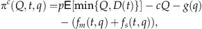1 where the first term is the expected revenue, the second term is the production cost, the third term is the cost of investment in quality improvement, and the last two terms are the total warranty costs. The objective of the central planner is

Lemma 1. The profit function of the centralized supply chain π ^c (Q, t, q) is concave in (Q, t, q).

By Lemma 1, given the defect rate q and the warranty period t, the optimal production quantity can be determined by the first‐order condition and is given as 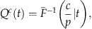2 which is increasing in t, as is increasing in t. A longer warranty period stimulates more demand, and hence the manufacturer orders more.

Substituting Q ^c(t) into (1), the resulting profit function depends only on q and t, and is a concave function. Hence, the optimal q ^c and t ^c are the solutions of 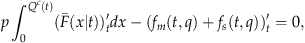3 and 4 where we note that g(q) is decreasing in q, whereas f _m(t, q) and f _s(t, q) are increasing in q and t. Denote the solution of (3) as t ^c(q) and that of (4) as q ^c(t). With a slight abuse of notation, the centralized solutions are t ^c=t ^c(q ^c), q ^c=q ^c(t ^c), and Q ^c=Q ^c(t ^c). Note that the defect rate q has an indirect impact on the ordering quantity through the warranty period.

Lemma 2.

(a)

π ^c (Q, t, q) is supermodular in (Q, t) and submodular in (t, q); and

(b)

Q ^c (t) is increasing in t; and t ^c (q) and q ^c (t) are decreasing in q and t, respectively.

From Topkis (1998), part (a) implies that the optimal production quantity Q ^c(t) increases in t. Moreover, from (1) and the submodularity of π ^c(Q, t, q) in (t, q), it is also clear that a longer warranty period leads to a lower defect rate and vice versa. Lemma 2 also demonstrates that the warranty period t and the defect rate q are two strategic substitutes in the centralized system.

Proposition 1. In the centralized supply chain,

(a)

both Q ^c and t ^c are decreasing in the unit production cost c, whereas the defect rate q ^c is increasing in c; and

(b)

both Q ^c and t ^c are increasing in the selling price p, whereas the defect rate q ^c is decreasing in p.

A higher unit production cost c means a lower margin for the supply chain and also a higher potential overstock cost. Therefore, the system tends to produce less and to offer a shorter warranty period. Furthermore, by Lemma 2, t and q are two strategic substitutes, and therefore the product defect rate q is higher. The impact of selling price p on the solution (Q ^c, t ^c, q ^c) is intuitive and can be similarly explained.

Lemma 3. Suppose there are two quality‐improvement schemes with costs g ₁ (q) and g ₂ (q), respectively. If (g ₁ (q))′≤(g ₂ (q))′, then q ₁ ^c ≥q ₂ ^c and t ₁ ^c ≤t ₂ ^c , where q _i ^c and t _i ^c are the optimal solutions under the cost function g _i (q), i=1,2.

This lemma states that if the marginal quality‐improvement cost becomes larger, then the resulting optimal defect rate q increases and the warranty period gets shorter.

4. Decentralized Supply Chain

In this section, we consider a decentralized supply chain in which the supplier and the manufacturer act to maximize their own profit. Recall that the manufacturer determines the ordering quantity, and the supplier controls product quality. We analyze two scenarios differentiated by which party determines the warranty period. The scenario where the manufacturer (supplier) determines warranty period is called the manufacturer (supplier) warranty. In each case, a game arises, as one party's decision affects that of the other. Recall that the product defect rate and the warranty period are set first, followed by the manufacturer's order. Hence, if the warranty period is determined by the supplier, then a Nash game arises between the supplier and the manufacturer.² If, in contrast, the warranty period decision is made by the supplier, then the game between the two becomes a pure Stackelberg game in which the supplier is the leader.

4.1 Manufacturer Warranty

In this subsection, the manufacturer decides the purchasing quantity Q and the warranty period t, and the supplier sets the product defect rate q. For the sake of brevity, we include only the decision variables of each party in their objective function. Hence, the manufacturer's problem is 5

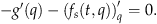
Determining only the defect rate, the supplier aims to solve the following problem: 6

According to the event sequence, when the manufacturer places his orders, the defect rate and the warranty period have already been set. So given any q and t, we first solve the optimal ordering quantity Q. It is not hard to see that π _m ^m(Q, t) is jointly concave in Q and t. Hence, the optimal Q ^d(t) is the solution of (π _m ^m(Q, t))_Q′=0 or 7

After we replace Q with Q ^d(t) in (5) and (6), the problem reduces to a Nash game on t and q between the manufacturer and the supplier. The concept of “Nash equilibrium” is used to represent a solution to this game, as both players simultaneously make their decisions (Fudenberg and Tirole 1991). A Nash equilibrium in this game is (t ^m, q ^m), such that neither firm wants to deviate from it unilaterally.

In the following notation, the operator “arg max” always refers to the largest maximizer of the objective function if there exists more than one. Define the supplier's best response as 8 and the manufacturer's best response

In addition, (t ^m, q ^m) is a Nash equilibrium if q ^m=q ^m(t ^m) and t ^m=t ^m(q ^m).

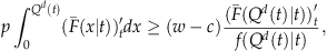
Note that π _m ^m(Q ^d(t), t) is concave in t and π _s ^m(q) is concave in q, and thus the best response t ^m(q) for the manufacturer is the solution of 9 and that for the supplier q ^m(t) is the solution of 10

The following result is parallel to Lemma 2 in the centralized case.

Lemma 4.

(a)

π _m ^m (Q, t) is supermodular in (Q, t); π _m ^m (Q ^d (t), t) and π _s ^m (q) are submodular in (t, q).

(b)

Q ^d (t) is increasing in t, and t ^m (q) and q ^m (t) are decreasing in q and t, respectively.

Lemma 4 states that if the manufacturer increases the protection period t, then the supplier's best response is to lower the defect rate q.

The next theorem is the key result of this section, as it shows the existence and uniqueness of a pure‐strategy Nash equilibrium for the game between the manufacturer and the supplier.

Theorem 1. In the game under a manufacturer warranty, there exists a unique pure‐strategy Nash equilibrium (t ^m , q ^m ), and the equilibrium ordering quantity is Q ^m =Q ^d (t ^m ).

We now provide comparative statics on the equilibrium solutions with respect to the cost parameters and the warranty cost share rate α.

Proposition 2. Under a manufacturer warranty,

(a)

both Q ^m and t ^m are decreasing in the wholesale price w, and the defect rate q ^m is increasing in w;

(b)

both Q ^m and t ^m are increasing in the selling price p, and the defect rate q ^m is decreasing in p; and

(c)

both Q ^m and t ^m are decreasing in the warranty cost share rate α, and the defect rate q ^m is increasing in α.

The results are intuitive. A higher wholesale price w implies a lower margin for the manufacturer and also a higher potential overstock cost. Therefore, the manufacturer tends to order less and to offer a shorter warranty period. Interestingly, the supplier produces lower‐quality products when she charges a higher wholesale price. This is the case because a higher wholesale price leads to a shorter t being set by the manufacturer, which, in turn, induces the supplier to set a higher defect rate q. The selling price p has an opposite effect on the solutions. When the selling price p increases, the manufacturer orders more to avoid a potential understock loss and offers a longer protection period t to stimulate more customer demand. Consequently, to avoid a high warranty cost, the supplier improves the quality of the product, i.e., decreases the defect rate q. Part (c) dictates that when the manufacturer shares more of the warranty cost, he tends to set a shorter equilibrium warranty period and to order less whereas the supplier responds by setting a higher defect rate.

4.2 Supplier Warranty

In this subsection, we analyze the case where the supplier determines both product quality and the warranty period, whereas the manufacturer only makes the ordering decision. Unlike the case in the previous section, the game between the manufacturer and the supplier here is a pure Stackelberg game in which the supplier is the leader, because the manufacturer places his order after the quality and warranty decisions have been made. The supplier's problem is thus 11

The manufacturer aims to solve 12

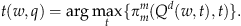
As the manufacturer is the follower, for any given warranty period t, the ordering quantity remains Q ^d(t), given by (7).

As the supplier can anticipate the manufacturer's ordering quantity, we can substitute ordering quantity Q with Q ^d(t) in (11). The resulting π _s ^s(t, q) remains concave in q. However, as Q ^d(t) may not be concave in t, the resulting π _s ^s(t, q) is not jointly concave in (t, q), in general. Nevertheless, the existence of a Stackelberg equilibrium (maximizer of π _s ^s(t, q)) is guaranteed by the compactness of the feasible domain. The next theorem summarizes the result.

Theorem 2. There exists at least one Stackelberg equilibrium (Q ^s , t ^s , q ^s ), where t ^s and q ^s are the solutions of 13 14 The equilibrium ordering quantity Q ^s =Q ^d (t ^s ).

Denote the solutions of (13) and (14) by t ^s(q) and q ^s(t), respectively, and so t ^s=t ^s(q ^s) and q ^s=q ^s(t ^s). We can observe from (14) that with a given t, the supplier sets the same defect rate q as in the manufacturer warranty case, i.e., q ^s(t)=q ^m(t). From the supermodularity of f _s(t, q), t ^s(q) is decreasing in q, and q ^s(t) is decreasing in t.

If the demand function D(t) is of a multiplicative form D(t)=d(t)ɛ or an additive form D(t)=d(t)+ɛ with d(t) being concave, then 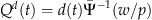or 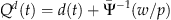, in which is the complementary cumulative distribution function of ɛ. We can then show that the profit function of the supplier π _s ^s(t, q) is strictly concave in (t, q), and thus the resulting Stackelberg equilibrium is unique.

We conclude this section with a discussion of the structural properties of the equilibrium solution and profit for the supplier and the manufacturer. As the effects of the wholesale and retail price, w and p, on the equilibrium solutions are, in general, ambiguous, we focus on the additive and multiplicative demand functions.

Proposition 3. In supplier warranty,

(a)

if the demand function is additive, then the equilibrium warranty period t ^s is increasing in w, and the ordering quantity Q ^s and the defect rate q ^s are decreasing in w; and

(b)

if the demand function is multiplicative, then both the manufacturer's order quantity Q ^s and the protection period t ^s are increasing in the selling price p, and the defect rate q ^s is decreasing in p.

Note that if the demand function is multiplicative, then the equilibrium solutions may not be monotonic in the wholesale price w (see the examples in section 6). Moreover, if the demand function is additive, then the equilibrium t ^s and q ^s become independent of p because the supplier's profit depends on p only through the ordering quantity set by the manufacturer, and the impact of t and p on that quantity is separable. This is different from the manufacturer warranty case. Another difference is that the product warranty t ^s increases and the defect rate q ^s decreases in w. When the supplier sets the warranty period, she offers a better quality product with a longer warranty if she charges a higher wholesale price.

It is unclear whether the equilibrium solutions have monotonic properties with respect to α in the supplier warranty. From (13) and (14), although we can show that both q ^s(t) and t ^s(q) are increasing in α, t ^s(q) is decreasing in q, and q ^s(t) is decreasing in t. So in general, at equilibrium, t ^s and q ^s may not be monotonic in α.

5. Comparison Between Centralized and Decentralized Chains

In this section, we compare the results of the centralized supply chain with those of the two decentralized systems. It is generally known that a centralized system always yields greater system‐wide profits than a decentralized system, which is the case in our model as well. However, it remains unclear which system provides a better quality product with a longer warranty period. We address the issue in the following.

Comparing the solutions of the centralized and decentralized systems, we obtain the following result.

Proposition 4.

(a)

If t ^c ≥t ^m , then Q ^c ≥Q ^m and q ^c ≤q ^m ; and

(b)

if t ^c ≥t ^s , then Q ^c ≥Q ^s and q ^c ≤q ^s.

If the centralized warranty period t ^c is shorter than that in the manufacturer warranty (supplier warranty), then the result in (a) ((b)) may not hold (see the numerical example in section 6). This implies that, in general, the centralized system may not always provide the best warranty or product quality. With a given t, it is clear that the centralized chain offers a lower defect rate due to the system‐wide consideration of warranty costs. However, when t is a decision variable in a decentralized chain, the warranty decision‐maker considers only his/her own warranty cost and therefore may set a longer warranty period, which can lead to better product quality. Hence, the centralized system may not always provide the longest product warranty period or best product quality.

We next compare the results for two decentralized warranty systems. We first explain that each firm wishes to make the warranty decision. Note that with given t both systems have the same ordering quantity Q ^d(t) and defect rate q ^m(t)=q ^s(t). The supplier's equilibrium profit in the two decentralized systems can be written as π _s ^s(t ^s, q ^s(t ^s)) and π _s ^m(q ^m(t ^m)), respectively. Because t ^s is optimized by the supplier, whereas t ^m is not, π _s ^s(t ^s, q ^s(t ^s))≥π _s ^m(q ^m(t ^m)). An analogous argument can show that the manufacturer also prefers to set the warranty. Therefore, without proper incentives, both firms will prefer to determine the warranty period themselves.

In the remainder of this section, we compare the equilibrium solutions of the two warranty systems. We find that the system parameters determine which warranty system leads to a longer warranty period and better product quality.

Proposition 5.

(a)

If α≤0.5 and 15 then t ^m ≥t ^s , Q ^m ≥Q ^s , and q ^m ≤q ^s.

(b)

If α>0.5 and 16 then t ^m <t ^s , Q ^m <Q ^s , and q ^m >q ^s.

Proposition 5 states that when the manufacturer shares less than half of the total warranty cost and has a higher marginal revenue with respect to the warranty period than the supplier, the manufacturer warranty leads to a longer warranty period and a lower defect rate than the supplier warranty. If, however, the manufacturer shares more than half of the total warranty cost and has a lower marginal profit than the supplier, then the product will be of better quality and have a longer warranty period under a supplier warranty.

To sharpen conditions (15) and (16) on the relationships between the solutions under the two warranty systems, we next analyze two special cases of the demand function: additive and multiplicative demand. Recall that the additive demand function is D(t)=d(t)+ɛ and the multiplicative demand function is D(t)=d(t)ɛ. We denote ψ(·) as the probability density function of ɛ.

For a multiplicative demand function, we obtain

It follows that, with a multiplicative demand function, condition (15) in Proposition 5 can be simplified to and condition (16) to

When the demand function is additive, we have and (15) is simplified to and (16) to

We can thus see that, with the additive demand function, when the manufacturer shares a smaller portion of the warranty costs and has a higher margin, he sets a longer protection period, and the product quality in the supply chain is better.

We can further obtain the following result for an additive demand function.

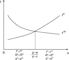
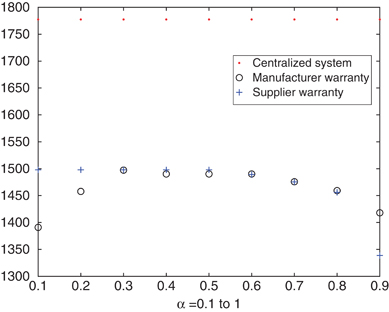
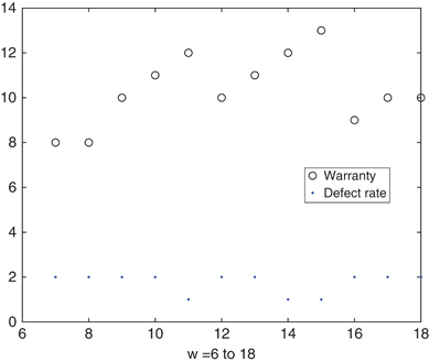
Corollary 1. When the demand function is additive, t ^m ≥t ^s , Q ^m ≥Q ^s , and q ^m ≤q ^s , if and only if

Figure 1 illustrates the equilibrium warranty periods with additive demand for two different warranty systems under different values of α. It can be seen that if α≤(p−w)/(p−c), then the manufacturer warranty offers a better quality product to customers than the supplier warranty; otherwise, customers are better off with the latter. The intersection point in Figure 1 means that if the total warranty cost is shared proportionally by the manufacturer and the supplier according to their margins, i.e., α=(p−w)/(p−c), then both warranties lead to the same equilibrium solutions. Such a situation might occur if both firms had similar degrees of bargaining power as sharing warranty costs in proportion to the two parties' margins leads to a “fair game.”

Figure 1

Equilibrium Warranty Periods with Additive Demand

The centralized supply chain is known to generate a higher level of overall profit than decentralized chains. So the supplier and the manufacturer could agree on certain cooperative strategies and, then, through a side payment or other type of contract, to achieve a mutually beneficial situation. The following supplier‐development and buy‐back contract is designed to coordinate the supply chain. Under such a contract, the supplier charges a unit wholesale price w, buys back any unsold items from the manufacturer at a unit price b and shares (1−λ) of the manufacturer's warranty cost, 0≤λ≤1; the manufacturer shares λ of the supplier's warranty and quality investment costs. Defining contract terms w and b as it is easy to show that the supplier‐development and buy‐back contract coordinates the supply chain, i.e., the decentralized and centralized solutions coincide. Moreover, the contract has sufficient flexibility to allow for any division of the supply chain's profit between the supplier and the manufacturer through parameter λ. The determination of λ usually depends on each player's bargaining power. We can use the Nash bargaining framework to determine λ (Nash 1953). If the two parties cannot reach an agreement on cooperation, then we assume their expected profit is given by the profit they would achieve under the manufacturer warranty, i.e., π _m ^m and π _s ^m. π _m ^m and π _s ^m represent the relative bargaining positions of the manufacturer and the supplier, respectively. 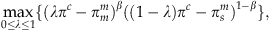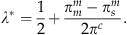The Nash bargaining solution solves the following problem: 17 where β represents the relative bargaining power of the manufacturer and 1−β that of the supplier. For simplicity, we assume that both parties have the same bargaining power, i.e., β=1/2, which yields the following Nash bargaining solution:

The solution is intuitive. If π _m ^m≥π _s ^m, or the manufacturer has a better bargaining position, then the manufacturer will obtain a larger share of the supply chain profit than the supplier and vice versa. It is also clear that λ ^* falls between 0 and 1, and each party is better off by implementing the Nash bargaining solution with the contract. It should also be noted that, although the supplier‐development and buy‐back contract can align the interests of the supplier and the manufacturer, it may be administratively burdensome because it requires both parties to reveal their costs, which is sometimes too demanding, especially when one party can gain an advantage by concealing such information.

6. Numerical Study

In this section, we conduct a numerical study to investigate which warranty system performs better for a decentralized supply chain and how the wholesale price affects the expected profit of the supplier and the manufacturer under each decentralized warranty system. We also examine the impact of warranty cost share rate α and demand variance.

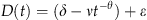
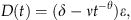
We use a specific form of the warranty cost function: f _total(t, q)=(at+bq)², with a, b≥0. For the investment in quality improvement, we let g(q)=c _q ln(q ₀/q), where c _q is a positive constant and q ₀ can be considered as the initial defect rate (see Porteus 1986, Zhu et al. 2007 for a similar quality‐improvement cost function). We consider both additive and multiplicative demand functions: and where δ, ν, and θ are positive constants. These functions can easily be shown to satisfy the conditions that we imposed in the previous sections.

The base example has the following parameters. For the warranty cost, a=3 and b=1. g(q) has parameters q ₀=70 and c _q=20. For the demand function D(t), δ=50, ν=10, and θ=0.5. Assume that ɛ is Poisson distributed with rate 4. The selling price p=20, the wholesale price w=10, and the unit production cost c=5. The feasible sets for q and t are [1, 60] and [1, 50], respectively.

The optimal solutions and profit of the centralized system with the aforementioned parameters are summarized in Table 1.

Table 1

Centralized Solutions

Additive demand					Multiplicative demand
t ^c	q ^c	Q ^c	π ^c	f _total ^c	t ^c	q ^c	Q ^c	π ^c	f _total ^c
2	1	46.93	538.61	49.00	3	1	175.91	1777.39	100.00

6.1 Warranty Cost Share Rate α

We first examine the impact of α, the proportion of the total warranty cost shared by the manufacturer. We vary the value of α from 0.1 to 0.9 with step size 0.1 and report the results in Tables 2 and 3. We observe that the resulting total warranty cost is smaller if the warranty is determined by the manufacturer and α is larger than 0.5. Q ^m and t ^m decrease, but q ^m increases, in α as we have shown analytically in Proposition 2(c), whereas t ^s and q ^s both increase in α in the examples we tested. These findings show that α has a different impact on the two warranty systems. More specifically, the manufacturer tends to set a shorter warranty when his share of the warranty cost α is higher, which results in the supplier offering poorer product quality. However, in the supplier warranty, when α increases (1−α decreases), the supplier bears less of the warranty cost and thus sets a longer warranty to boost customer demand, but produces products with a higher defect rate q ^s. The benefit from increasing t and q outweighs the resulting warranty cost, of which the manufacturer shares a larger portion. In Table 2, the additive demand case, when α≤0.5, as p−w=10 > w−c=5, we can also see that the manufacturer warranty results in products of better quality with a longer warranty period, which is consistent with our analytical result.

Table 2

Decentralized Solutions: Additive Demand

α	Manufacturer warranty						Supplier warranty
α	t ^m	q ^m	Q ^m	π _m ^m	π _s ^m	f _total ^m	t ^s	q ^s	Q ^s	π _m ^s	π _s ^s	f _total ^s
0.2	3	1	47.23	429.10	71.16	100.00	1	2	43.00	403.39	123.89	25.00
0.5	2	2	45.93	404.60	126.54	64.00	1	3	43.00	390.39	134.00	36.00
0.8	1	6	43.00	343.59	149.67	81.00	2	5	45.93	339.80	152.66	121.00

Table 3

Decentralized Solutions: Multiplicative Demand

α	Manufacturer warranty						Supplier warranty
α	t ^m	q ^m	Q ^m	π _m ^m	π _s ^m	f _total ^m	t ^s	q ^s	Q ^s	π _m ^s	π _s ^s	f _total ^s
0.2	4	1	135.00	1003.00	454.83	169.00	2	2	128.79	976.29	521.63	64.00
0.5	3	2	132.68	958.48	531.79	121.00	2	2	128.79	957.09	540.83	64.00
0.8	2	5	128.79	892.29	566.95	121.00	3	4	132.68	883.78	572.35	169.00

In the preceding analysis, we noted that the centralized system may not always provide the longest warranty, which we can also see from the numerical examples in Tables 1–3. When α=0.2, for additive demand, the warranty period under the manufacturer warranty is longer and the optimal ordering quantity is larger relative to the centralized system.

Figure 2 illustrates the supply chain's profit under centralized and decentralized control. It can be observed that if the warranty is determined by the firm that shares more of the warranty cost, then the entire supply chain generates more profit. Furthermore, having the right decision‐maker for the warranty can significantly increase total supply chain profits. For example, in the additive demand case with α=0.2, if the supplier rather than the manufacturer sets the warranty, then the total supply chain profit increases by 5.4% (=). Thus, allowing the firm with the larger share of the warranty cost to determine the warranty tends to render the entire supply chain better off.

Figure 2

Centralized and Decentralized Supply Chain Profit

6.2 Demand Variance

To investigate the impact of demand variance on the supply chain, we let ɛ follow a negative binomial distribution with fixed mean value , and increase its variance var[ɛ] linearly from 5 to 45 with step size 10. The results for centralized and decentralized systems are presented in Tables 4–6.

Table 4

Centralized Solutions

var[ɛ]	Additive demand					Multiplicative demand
var[ɛ]	t ^c	q ^c	Q ^c	π ^c	f _total ^m	t ^c	q ^c	Q ^c	π ^c	f _total ^s
5	3	1	176.91	1696.60	100.00	2	1	171.72	528.34	49.00
15	2	1	214.64	1273.97	49.00	1	2	200.00	419.70	25.00
25	2	1	214.64	959.96	49.00	1	2	200.00	331.36	25.00
35	2	1	171.72	700.33	49.00	1	2	160.00	262.18	25.00
45	2	1	171.72	545.20	49.00	1	2	160.00	208.62	25.00

Table 5

Decentralized Solutions under Different Demand Variances: Additive Demand

var[ɛ]	Manufacturer warranty						Supplier warranty
var[ɛ]	t ^m	q ^m	Q ^m	π _m ^m	π _s ^m	f _total ^m	t ^s	q ^s	Q ^s	π _m ^s	π _s ^s	f _total ^s
5	2	3	128.79	378.17	134.25	81.00	1	4	120.00	369.73	138.16	49.00
15	2	3	85.86	266.17	129.25	81.00	1	4	80.00	264.64	133.16	49.00
25	1	4	40.00	177.63	128.16	49.00	1	4	40.00	177.63	128.16	49.00
35	1	4	40.00	112.92	128.16	49.00	1	4	40.00	112.92	128.16	49.00
45	1	4	40.00	61.73	128.16	49.00	1	4	40.00	61.73	128.16	49.00

Table 6

Decentralized Solutions under Different Demand Variances: Multiplicative Demand

var[ɛ]	Manufacturer warranty						Supplier warranty
var[ɛ]	t ^m	q ^m	Q ^m	π _m ^m	π _s ^m	f _total ^m	t ^s	q ^s	Q ^s	π _m ^s	π _s ^s	f _total ^s
5	3	2	132.68	884.72	543.89	121.00	2	3	128.79	880.63	548.54	81.00
15	2	3	85.86	424.95	333.89	81.00	2	3	85.86	424.95	333.89	81.00
25	1	4	40.00	172.58	123.16	49.00	1	4	40.00	172.58	123.16	49.00
35	1	4	40.00	109.45	123.16	49.00	1	4	40.00	109.45	123.16	49.00
45	1	4	40.00	59.50	123.16	49.00	1	4	40.00	59.50	123.16	49.00

We find that the system profit of the centralized supply chain, the optimal profit of each firm in the decentralized systems, and the total warranty costs all decrease as var[ɛ] increases. With respect to the ordering quantity, the centralized solution is not monotonic, whereas both decentralized systems order less when var[ɛ] increases. In addition, the optimal warranty periods decrease, and the defect rates increase, in var[ɛ]. In general, we can thus conclude that a higher var[ɛ] deteriorates system performance.

6.3 Wholesale Price w

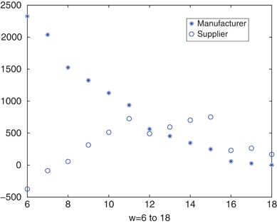
The wholesale price w plays an important role in the supply chain. Hence, we investigate its impact on the profit of each firm as well as on that of the entire system. We use a different multiplicative demand function D(t)=30(ln t)ɛ, where ɛ remains Poisson distributed with mean 4.

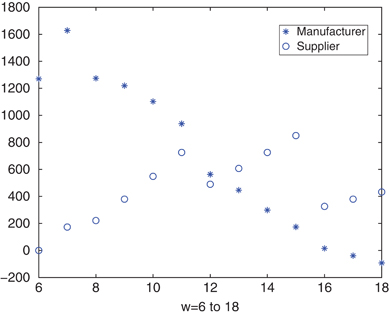
We depict the profits of the supplier and the manufacturer for different values of w under the manufacturer and supplier warranty in Figures 3 and 4, respectively. From Figure 3, it is clear that the supplier's profit is not monotonic in w, whereas the manufacturer's profit is decreasing in w (one can actually show this result analytically). This implies that a higher wholesale price will render the manufacturer worse off but may not benefit the supplier, mainly because the manufacturer will react to the price increase by ordering fewer product units. This response is caused not only by the higher unit wholesale price but also by the resulting shorter warranty period set by the manufacturer, which further depresses customer demand. Figure 4 shows that under the supplier warranty, the manufacturer does not necessarily suffer from a high wholesale price, probably because when the supplier charges a higher w, she may also offer better product quality and a longer warranty period. Doing so stimulates customer demand and possibly results in a lower warranty cost; thus, the manufacturer may benefit even though his unit margin is squeezed. This result is different from those for systems without quality and warranty issues. It further suggests that squeezing the profit margin of the supplier (manufacturer) does not necessarily benefit the manufacturer (supplier). This non‐monotonicity of profits in the wholesale price was also reported in Lariviere and Porteus (2001), albeit under a different model setting.

Figure 3

Equilibrium Profit: Manufacturer Warranty

Figure 4

Equilibrium Profit: Supplier Warranty

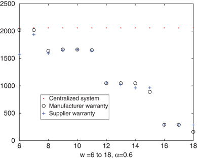
The total supply chain profit under different w values is illustrated in Figure 5, from which it can be observed that, although the total profit of the entire system is not monotonic in the wholesale price, it has a clear decreasing trend. Hence, charging a high wholesale price amplifies the double marginalization effect and worsens the performance of the entire system. Moreover, Figure 6 illustrates that the equilibrium solutions under the supplier warranty may not be monotonic in the wholesale price w for the multiplicative demand case, which is stated in the discussion following Proposition 3.

Figure 5

Centralized and Decentralized Supply Chain Profit

Figure 6

Equilibrium Warranty and Defect Rate under Supplier Warranty

7. Extensions

We here discuss several extensions to the model presented in the previous section. Our aim is to show how the analysis and results can be generalized to situations where the supplier also needs to decide the wholesale price, the production cost depends on product quality, and customer demand depends on both the warranty policy and product quality.

7.1 Endogenous Wholesale Price

In this subsection, we extend the model to the case where the supplier also needs to decide the wholesale price w. This change does not affect our analysis of the centralized solutions and so we merely consider the decentralized setting. We still consider the manufacturer warranty and the supplier warranty separately.

Under the manufacturer warranty, the supplier's aim is to solve the following problem: 18 and the manufacturer's problem is the same as (5). It is reasonable to assume that the wholesale price w is set when t and q are determined, but before the ordering quantity Q is decided. Hence, given any w, t, and q, the optimal ordering quantity has the same structure as (7). However, to signify its dependency on w, we denote it by Q ^d(w, t). After we replace Q with Q ^d(w, t) in (5) and (18), the problem reduces to a Nash game on t and (w, q) between the manufacturer and the supplier. A Nash equilibrium in this game is (w ^m, t ^m, q ^m), from which neither firm wants to unilaterally deviate.

Define the supplier's best response as and the manufacturer's best response as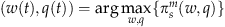

Also (w ^m, t ^m, q ^m) is a Nash equilibrium if w ^m=w(t ^m), q ^m=q(t ^m), and t ^m=t(w ^m, q ^m).

It is not difficult to see from (18) that w and q are two separable decisions for each given t. Thus, we first solve the best response w(t) given in the following result.

P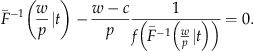roposition 6. If the demand distribution F(x|t) has an increasing failure rate (IFR) in x, then (w−c)Q ^d (w, t) is quasi‐concave in w, and thus the optimal response w(t) satisfies 19

Because π _m ^m(Q ^d(w, t), t) is concave in t and π _s ^m(w, q) is separable and quasi‐concave in w and concave in q, the best responses t(w, q) and q(t) are still given by (9) and (10).

The next theorem obtains the existence of a pure‐strategy Nash equilibrium for the game between the manufacturer and the supplier.

Theorem 3. Under the manufacturer warranty, if the demand distribution F(x|t) has an IFR in x, then there exists a pure‐strategy Nash equilibrium (w ^m , t ^m , q ^m ), and the equilibrium ordering quantity Q ^m=Q ^d (w ^m , t ^m ).

Although we can still show the existence of a pure‐strategy Nash equilibrium, its uniqueness is quite challenging to establish after the wholesale price w is incorporated as a decision variable.

We next consider the supplier warranty case. Here, the game between the manufacturer and the supplier is again a pure Stackelberg game in which the supplier is the leader. The supplier's problem is 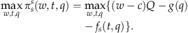20

As the manufacturer is the follower, with any given warranty period t and wholesale price w, the ordering quantity Q remains Q ^d(w, t). As the supplier can anticipate the ordering quantity set by the manufacturer, we can substitute Q with Q ^d(w, t) in (20), and the resulting π _s ^s(w, t, q) is quasi‐concave in w and concave in q, but may not be concave in t. Nevertheless, the existence of a Stackelberg equilibrium is guaranteed by the compactness of the feasible domain (note that w∈[c, p]). The next theorem summarizes the result.

T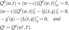heorem 4. There exists at least one Stackelberg equilibrium (w ^s , Q ^s , t ^s , q ^s ), where w ^s , Q^s, t ^s , and q ^s are the solutions of 21

7.2 Quality‐Dependent Production Cost

In certain production processes, the production cost is related to the product's quality level. Producing a better quality product often requires a higher production cost. Denote the production cost at the supplier by c(Q, q), which is decreasing in q, increasing in Q and jointly convex in (Q, q).

With this more general production cost function, the expected profit of the integrated supply chain becomes 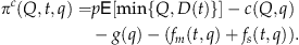22

It is not difficult to see that π ^c(Q, t, q) remains concave in (Q, t, q). But the optimal solutions become slightly more difficult to solve, as they are now the solutions of the following system of equations: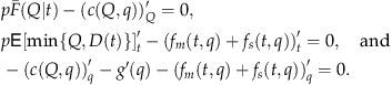

Denote the solution of the first equation above by Q ^c(t, q). As the production cost depends on the defect rate q, the optimal production quantity depends explicitly on both product quality and the warranty period. We further assume that c(Q, q) is submodular in (Q, q), which is intuitive in that a lower defect rate should lead to a higher marginal production cost (c(Q, q))′_Q. As a result, π ^c(Q, t, q) is supermodular in (Q, q). Because π ^c(Q, t, q) is still supermodular in (Q, t), the centralized production quantity Q ^c(t, q) increases with t and q. In addition, the submodularity of π ^c(Q,\xE2\x80\x83t, q) on (t, q) continues to hold here. The centralized warranty period therefore becomes longer if product quality improves.

In the manufacturer warranty case, the optimal ordering quantity with a given t is independent of q and is the same as (7). We can still show that the expected profit function π _m ^m(Q ^d(t), t) is concave in t, and, after replacing cQ with c(Q, q) in the supplier's objective function (6), π _s ^m(q) is concave in q. Moreover, both π _m ^m(Q ^d(t), t) and π _s ^m(q) are submodular in (t, q), as c(Q, q) is submodular and is increasing in t. Hence, we are still able to show that there exists a unique pure‐strategy Nash equilibrium (t ^m, q ^m).

Theorem 5. If c(Q, q) is jointly convex in (Q, q), then there exists a unique pure‐strategy Nash equilibrium (t ^m , q ^m ), and the optimal production quantity is Q ^d (t ^m ).

In the supplier warranty case, the supplier's problem becomes 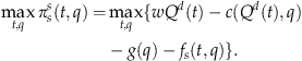23

With the current condition (the monotonicity and convexity of c(Q, q)), π _s ^m(t, q) remains concave in q, but may not be jointly concave in (t, q) even with additive or multiplicative demand functions. However, there still exists at least one Stackelberg equilibrium, as the feasible domains of q and t are compact.

7.3 Quality‐Dependent Demand

In this subsection, we generalize our demand function to the case in which customer demand depends not only on the warranty period t but also on the defect rate q. To obtain more analytical results, we adopt an additive demand function (although similar results can be derived with a multiplicative demand function), D(t, q)=d(t, q)+ɛ, in which d(t, q) is increasing in t and decreasing in q, as a longer warranty period or a lower defect rate should generate more demand. We also assume that d(t, q) is strictly joint concave and supermodular in (t, q). Our supermodularity assumption can be justified by the following argument. If customers know the quality of the product, then a marginal increase in the warranty period will have a smaller positive impact on demand when the defect rate is small.

For the centralized supply chain, the profit function π ^c(Q, t, q) can be shown still concave in (Q, t, q) because d(t, q) is jointly concave. Under additive demand, 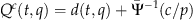and Q ^c(t, q) is increasing in t but decreasing in q. After substituting Q ^c(t, q) into π ^c(Q, t, q), the optimal centralized solutions (t ^c, q ^c) can be derived using the set of first‐order conditions. The submodularity of π ^c(Q, t, q) in (t, q) may not hold, as d(t, q) is supermodular in (t, q). Therefore, in this case, a longer warranty does not always imply a lower defect rate at the optimum.

Now we consider the decentralized setting. Under the manufacturer warranty, as the joint concavity of π _m ^m(Q, t) still holds, we obtain the optimal order quantity Q ^d(t, q) as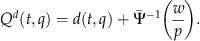

In addition, the equilibrium warranty period and defect rate are determined by the following two equations: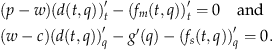

The following theorem states the existence and uniqueness of a pure‐strategy Nash equilibrium under the manufacturer warranty scenario.

Theorem 6. When the demand function is given by D(t, q)=d(t, q)+ɛ, in the manufacturer warranty, there exists a unique pure‐strategy Nash equilibrium (t ^m , q ^m ), and the equilibrium ordering quantity is Q ^m =Q ^d (t ^m , q ^m ).

Because of the loss of submodularity for π _m ^m(Q, t) and π _s ^m(q) in (t, q), the effects of the wholesale price w and the retail price p on the equilibrium solutions and equilibrium profit are ambiguous.

For the supplier warranty, it is not hard to show that after substituting Q ^d(t, q) into the supplier's objective function π _s ^s(t, q), the resulting function is jointly concave in (t, q) (note that we consider additive demand here). So we can easily solve the Stackelberg equilibrium. However, results similar to Proposition 3 do not hold when demand also depends on the defect rate.

8. Conclusion

We study a single‐period, two‐echelon supply chain model with product quality and warranty protection period decisions in this paper. Both centralized and decentralized systems are analyzed, with a particular focus on two decentralized cases: the manufacturer warranty and the supplier warranty. We analyze the game behavior of both the supplier and the manufacturer and derive the equilibrium strategies. Our results show that the warranty cost share rate between the two firms has different impacts on the equilibrium solutions under the manufacturer and supplier warranties. When the manufacturer shares less (more) of the warranty cost and has a higher (lower) marginal profit, he is likely to set a longer (shorter) warranty period and the resulting product quality determined by the supplier is likely to be better (worse). At the same time, our numerical results illustrate that if the product warranty is set by the firm sharing more of the warranty costs, then the total supply chain profit tends to be higher. We also observe that when the product quality and warranty period decisions are integrated in supply chain management, it may not be advantageous for firms to squeeze their supply chain partner's profit margin. In addition, to achieve supply chain coordination, we design a supplier‐development and buy‐back contract with sufficient flexibility to allow for any division of the supply chain's profit between the supplier and the manufacturer. We consider several extensions, including an endogenous wholesale price, quality‐dependent production costs and quality‐dependent demand.

This paper is by necessity limited in scope, and its coverage could be fruitfully extended in a number of interesting directions in future studies. First, we assume the product's selling price to be exogenous. If customer demand depends on both the warranty period and price, then how will the analysis and results in this paper change? This extension may require additional assumptions on the demand function for tractability. Second, our model could also be extended to a one‐supplier, multi‐manufacturer setting in which each manufacturer faces random demand and makes stocking quantity and warranty decisions simultaneously. Each manufacturer's customer demand depends on both his own and other manufacturers' warranty policies. Based on this model, a further potential avenue of research would be to investigate games among multiple competing manufacturers and between the supplier and the manufacturers. Third, our model and analysis mainly focus on non‐cooperative decision‐making between two firms. Various settings under a cooperative game framework are also important and would certainly be worth investigating. Finally, extending the current static setting to a dynamic setting with a sales‐dependent warranty cost would yield interesting insights, although it would be significantly more challenging.

Footnotes

Acknowledgments

We thank the Senior Editor and three anonymous referees for their helpful comments and suggestions. The first and third authors are supported in part by National Natural Science Foundation of China (NSFC) under no. 70832002, no. 70771028, and no. 70971024. The second author is supported in part by the Chinese University of Hong Kong Direct Grant under no. 2050372.

1

Consumers' prior knowledge also influences their evaluation of product quality when using warranty information (), but this issue is beyond the scope of this paper.

2

This is actually a two‐stage game in which the manufacturer orders in the second stage. As we shall see, however, the optimal ordering quantity can be first solved easily with given q and t, and thus the game is simplified to a Nash game.

References

Allen

2001. Lean: A supplier's weapon against warranty costs. Manuf. Eng. June.

Boulding

Kirmani

. 1993. A consumer‐side experimental examination of signaling theory: Do consumers perceive warranties as signals of quality? J. Consum. Res. 20 (1): 111–123.

Cachon

2003. Supply chain coordination with contracts. Graves

de Kok

eds. Handbooks in Operations Research and Management Science: Supply Chain Management. North Holland, Amsterdam, 229–239.

Cachon

Netessine

. 2004. Game theory in supply chain analysis. Simchi‐Levi

S. D.

Shen

Z. J.

eds. Handbook of Quantitative Supply Chain Analysis: Modeling in the eBusiness Era. Kluwer, Massachusetts.

Chao

G. H.

Iravani

S. M. R.

Savaskan

R. C.

. 2009. Quality improvement incentives and product recall cost sharing contracts. Manage. Sci. 55 (7): 1122–1138.

Chen

Yao

Zheng

. 1998. Quality control for products supplied with warranty. Oper. Res. 46 (1): 107–115.

Fudenberg

Tirole

. 1991. Game Theory. MIT Press, Cambridge, MA.

Glickman

T. S.

Berger

P. D.

. 1976. Optimal price and protection period decisions for a product under warranty. Manage. Sci. 22 (12): 1381–1390.

Guo

2009. Quality disclosure formats in a distribution channel. Manage. Sci. 55 (9): 1513–1526.

10.

W. T.

2008. Supply chain coordination contracts with free replacement warranty. Ph.D. dissertation, Drexel University.

11.

Lariviere

M. A.

Porteus

E. L.

. 2001. Selling to the newsvendor: An analysis of price-only contracts. Manuf. Serv. Oper. Manage. 3: 293–305.

12.

Chhajed

Mallik

. 2009. Design of extended warranties in supply chains. Working paper, University of Illinois at Urbana‐Champaign, IL.

13.

Lim

W. S.

2001. Producer‐supplier contracts with incomplete information. Manage. Sci. 47 (5): 709–715.

14.

Murthy

D. N. P.

Blischke

W. R.

. 1992. Product warranty management‐III: A review of mathematical models. Eur. J. Oper. Res. 63 (1): 1–34.

15.

Nash

J. F.

1953. Two person cooperative games. Econometrica 21 (1): 128–140.

16.

Padmanabhan

Rao

R. C.

. 1993. Warranty policy and extended service contracts: Theory and an application to automobiles. Mark. Sci. 12 (3): 230–247.

17.

Porteus

E. L.

1986. Optimal lot sizing, process quality improvement and setup cost reduction. Oper. Res. 34 (1): 137–144.

18.

Porteus

E. L.

1990. The impact of inspection delay on process and inspection lot sizing. Manage. Sci. 36 (8): 999–1007.

19.

Purohit

Srivastava

. 2001. Effect of manufacturer reputation, retailer reputation, and product warranty on consumer judgments of product quality: A cue diagnosticity framework. J. Consum. Psychol. 10 (3): 123–134.

20.

Reyniers

D. J.

Tapiero

C. S.

. 1995a. The delivery and control of quality in supplier‐producer contracts. Manage. Sci. 41 (10): 1581–1589.

21.

Reyniers

D. J.

Tapiero

C. S.

. 1995b. Contract design and the control of quality in a conflictual environment. Eur. J. Oper. Res. 82 (2): 373–382.

22.

Rosenblatt

M. J.

Lee

H. L.

. 1986. Economic production cycles with imperfect production process. IIE Trans. 18 (1): 48–55.

23.

Srivastava

Mitra

. 1998. Warranty as a signal of quality: The moderating effect of consumer knowledge on quality evaluations. Mark. Lett. 9 (4): 327–336.

24.

Starbird

S. A.

1997. Acceptance sampling, imperfect production, and the optimality of zero defects. Nav. Res. Logist. Q. 44 (6): 515–530.

25.

Tagaras

Lee

H. L.

. 1996. Economic models for vendor evaluation with quality cost analysis. Manage. Sci. 42 (11): 1531–1543.

26.

The PC Guide

2008. Warranty coverage: Retail, OEM and stolen drives. The PC Guide, 2008.

27.

Thomas

Rao

. 1999. Warranty economic decision models: A summary and some suggested directions for future research. Oper. Res. 47 (6): 807–820.

28.

Topkis

D. M.

1998. Supermodularity and Complementarity. Princeton University Press, Princeton, NJ.

29.

Tsay

A. A.

Nahmias

Agrawal

. 1999. Modeling supply chain contracts: A review. Tayur

Ganeshan

Magazine

eds. Quantitative Models for Supply Chain Management, vol. 17 of International Series in Operations Research and Management Science. Kluwer, Massachusetts, 299–336.

30.

Udell

J. G.

Anderson

E. E.

. 1968. The product warranty as an element of competitive strategy. J. Mark. 32 (4): 1–8.

31.

C. C.

Lin

P. C.

Chou

C. Y.

. 2006. Determination of price and warranty length for a normal lifetime distributed product. Int. J. Prod. Econ. 102 (1): 95–107.

32.

Zhu

Zhang

R. Q.

Tsung

. 2007. Pushing quality improvement along supply chains. Manage. Sci. 53 (3): 421–436.