
Abstract
For firms remanufacturing their products, the total life‐cycle costs and revenues from new and remanufactured products determine their profitability. In many firms, manufacturing/sales and remanufacturing/remarketing operations are carried out in different divisions. Each division is responsible for only part of the product's life cycle. Practices regarding transfer pricing across divisions vary significantly among companies, affecting the life‐cycle profit performance of the product. In this research, we identify characteristics of transfer prices that achieve the firm‐wide optimal solution. To this end, we consider a manufacturer who also undertakes remanufacturing operations and we focus on price (quantity) decisions. We determine that a cost allocation mechanism that allocates a portion of the initial production cost to each of the two stages of the product life cycle should be used. We also conclude that cost allocation should be implemented as a fixed cost allocation, where charges to the remanufacturing division should be determined independently of the actual quantity of units remanufactured.
1. Introduction
Remanufacturing is a process by which value is recovered from used products. In this note, we focus on a firm that manufactures and sells a new product, and subsequently remanufactures and remarkets the same product. Such a firm needs to make two distinct quantity decisions for the new and the remanufactured products. Because sales of new products determine the supply of remanufactured ones in the future, the two quantity decisions are linked. However, the division responsible for the production/sales of the new products is typically different from the one in charge of remanufactured products. Examples of such firms are easily found; they include Hewlett Packard (Guide and Van Wassenhove 2002), Bosch (Valenta 2004), DaimlerChysler (Driesch and Flapper 2005), and Océ (Zuidwijk et al. 2005).
The natural question arising for such firms is because the same inputs (materials, parts, etc.) may be used twice to generate revenues in different divisions, who should bear the cost of these inputs? The accounting mechanism that prices the internal transfers of goods or services across different divisions within the firm, where the output from one division becomes an input into another, is transfer pricing. A wide variety of transfer pricing practices between the divisions responsible for manufacturing and remanufacturing exist in practice. These approaches reflect a lack of consensus concerning the value of a used product. A non‐exhaustive list of contrasting examples follow 1 :
No manufacturing cost allocated to remanufacturing. In this approach, the manufacturing division bears the full cost of manufacturing the new product. Once the product is returned, the remanufacturing division is not charged any cost for using this input. This approach reflects the view that once the product is manufactured, the manufacturing cost becomes entirely sunk, therefore, the firm should not take it into account in subsequent decisions. Full manufacturing cost allocated to remanufacturing. In this approach, the remanufacturing division is charged the entire cost of the initial production, reflecting the view that the division is using a costly input. Interestingly, the manufacturing division has already been charged the same cost, so from the firm's perspective, this approach amounts to double counting. Partial manufacturing cost allocated to remanufacturing. In this approach, an internal transfer price lower than the initial production cost is posted and the sales organization decides how many products to return for remanufacturing at the said price, and how many units to scrap (Zuidwijk et al. 2005).
Which of these approaches, if any, is appropriate? While there is an extensive economic and accounting literature on transfer pricing (Edlin and Reichelstein 1995, Vaysman 1998), this literature offers no guidance specific to closed‐loop supply chains. In the operations literature, the only papers that raise a related issue—that of inventory valuation for remanufacturable products—are Teunter et al. (2000), Teunter (2001), and Teunter and van der Laan (2002, 2004). These papers develop appropriate holding costs for returned products in decision support systems based on average cost models; their focus is inventory valuation for centralized decision making. The operations literature on remanufacturing makes the implicit assumption that optimal prices for the two products will be reached (Atasu et al. 2008, Debo et al. 2005, Ferguson and Toktay 2006, Ferrer and Swaminathan 2006, Groenevelt and Majumder 2001, Savaşkan et al. 2004). In practice, where different divisions and different decision makers are involved, the effectiveness of different transfer pricing methods becomes relevant.
Given the discord among existing transfer pricing approaches in practice, in conjunction with the lack of academic research, there is a clear need for specific transfer pricing guidelines in closed‐loop supply chains. The goal of this note is to provide such guidelines. Specifically, we investigate the following: Is there is a coordinating transfer price mechanism? If so, what are its properties?
2. The Model
To address these research questions, we develop a model with the following features:
Firm structure: As discussed in the introduction, a decentralized structure is prevalent in firms that undertake both manufacturing and remanufacturing operations. To capture this, in our model, division D1 incurs the manufacturing cost and determines the new product's sales price. Revenues from the new product sales accrue to this division. In firms where the manufacturing division is operated as a cost center, D1 can be viewed as the new product sales organization, which is charged the unit standard manufacturing cost for each new unit produced by manufacturing. Division D2 then remanufactures some used products and salvages the rest. The respective managers of these divisions will be referred to as M1 and M2.
Performance evaluation: For incentive purposes, the divisional profit is the most important in evaluating the divisional manager's performance and compensation. In the accounting literature, this is called responsibility accounting, where the appropriate performance measure should evaluate the results within the domains of the manager's responsibility. For these reasons, we focus on the divisional profit as the performance measure for divisional managers. In practice, some firms may treat remanufacturing as a cost center instead of an activity that can create value for the company despite the shortcomings of this approach (Blackburn et al. 2004). Our research prescribes how firms that have already made this strategic shift vis‐à‐vis their remanufacturing operations should structure internal transfer prices to realize its potential.
Information structure: The model considered is under perfect information. In the absence of asymmetric information, when both communication and contracting are costless, having decisions made centrally and implemented by the divisions is the first‐best decision‐making structure. At the same time, modern firms of a certain size tend to be decentralized, i.e., decision rights are delegated to divisional managers, when the economic environment is too complex and making decisions centrally may no longer be efficient. The remanufacturing setting is typically characterized by the above conditions, which motivates our modeling choice. Modifications would be necessary to the transfer pricing mechanism if divisional managers are endowed with private information about costs or demands.
Market characteristics: We assume that the new and remanufactured products are sold to different market segments that do not overlap such that there is no cannibalization between the products. This is appropriate when the remanufactured product is sold in a different geographic region, or when the customers in these segments have distinct preferences. Specifically, firms can limit cannibalization by selling through different channels (Guide and Van Wassenhove 2002), or by remanufacturing only a subset of their product line where they believe cannibalization effects are limited (Valenta 2004).
Product life cycle: We assume that the new product can be used for only one period. Subsequently, products are returned by customers. A fraction q∈[0, 1] of returned products can be remanufactured once; the rest cannot be used and will be scrapped. Remanufactured products also have a one‐period lifetime, after which they are disposed of. Similar assumptions are adopted in other papers, e.g., Groenevelt and Majumder (2001), Debo et al. (2005), and Ferguson and Toktay (2006). With the above assumptions, it is sufficient to analyze a two‐period model. Only new products are sold in the first period by manufacturing, and only remanufactured products are sold in the second period by remanufacturing.
Consumer Characteristics: We assume that consumer willingness‐to‐pay is heterogeneous and uniformly distributed in the interval [0, 1]. The market size is normalized to 1. Consumers typically value the remanufactured product less than the new product (Agrawal et al. 2010, Guide and Li 2010, Subramanian and Subramanyam 2010). We model this by letting a consumer of type φ∈[0, 1] have a willingness‐to‐pay of φ for a new product and (1−δ)φ for a remanufactured product. The parameter δ is “perceived depreciation.” The utility each consumer derives from purchasing a product is equal to the difference between his willingness to pay and the product price. We let p n and d n denote the (first period) new product price and demand, and p r and d r the (second period) remanufactured product price and demand. Then p n =1−d n and p r =(1−δ) (1−d r ).
The cost structure: We denote the unit manufacturing cost by c; and the unit remanufacturing cost by c r . Second‐period profits are discounted by β<1. Returned remanufacturable products have salvage value s per unit. The disposal cost for non‐remanufacturable units is zero.
3. Coordinating Cost Allocation
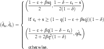
We first establish the firm‐wide profit maximizing solution to use as a benchmark. Because of the one‐to‐one correspondence between price and demand, the optimization problem can be formulated either in terms of prices or demands. We proceed with the latter for ease of interpretation. The optimal demand levels are those that maximize the present value of the profits from both periods subject to an availability constraint: 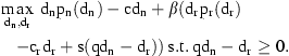
 and
and  .
.
L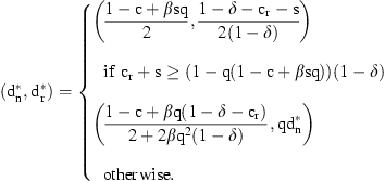
We next propose a cost allocation scheme where a fraction α of the unit manufacturing cost is charged to manufacturing, and the rest, 1−α, to remanufacturing, for each unit manufactured by manufacturing. Thus, M1 maximizes (p n −αc)d n and M2 maximizes −(1−α)cd n +d r p r (d r )−c r d r +s(qd n −d r ). s.t. d r ≤qd n , where d n has already been chosen by M1.
L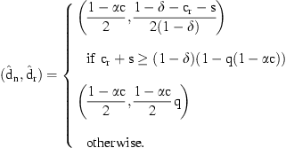
P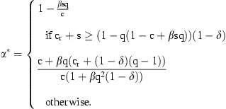
Note that under the cost allocation scheme  , we obtain demand levels that are exactly the same as the benchmark demand levels
  . In other words, we have shown that a proportional cost allocation scheme with α not necessarily equal to 1 achieves the centralized benchmark.
2
This is consistent with the literature on capital investments, where the incentives of the division making the investment are aligned with those of the firm by allocating part of the cost of the investment to other divisions (Wei 2004) or by spreading it over time to reflect its pattern of future potential benefits. These allocation schemes are developed for capital investments; this concept has not been previously proposed on a production cost basis.
. In other words, we have shown that a proportional cost allocation scheme with α not necessarily equal to 1 achieves the centralized benchmark.
2
This is consistent with the literature on capital investments, where the incentives of the division making the investment are aligned with those of the firm by allocating part of the cost of the investment to other divisions (Wei 2004) or by spreading it over time to reflect its pattern of future potential benefits. These allocation schemes are developed for capital investments; this concept has not been previously proposed on a production cost basis.
The logic behind the expression for  is not immediately apparent. We interpret this result next. Let C(d
n
) denote the effective cost to the firm of producing d
n
units.
is not immediately apparent. We interpret this result next. Let C(d
n
) denote the effective cost to the firm of producing d
n
units.
P .
.
This proposition states that in both cases of Proposition 1, the expression obtained for  is such that the cost allocated to the manufacturing division equals the marginal cost to the firm evaluated at
  .
.
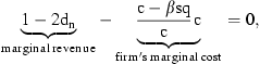
Let us discuss  , the case with ample supply of used remanufacturable products; the other case follows the same logic. Rewriting
  as c−βsq, we see that this quantity is the marginal cost of producing a new product to the entire firm when the next unit will be salvaged (because there is already sufficient supply).
When we allocate only  portion of the production cost to M1 in the first period, he makes the following calculation:
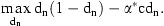
 , the optimal production quantity of new products. M1 always chooses the quantity that makes his marginal revenue equal to his marginal cost. His marginal revenue is already equal to that of the firm's. By changing his marginal cost from c to
  , we are able to incorporate the firm‐wide incentives into his performance measure.
For the other case,  can again be interpreted as the marginal cost of producing one more new product at
  , but this time when the next unit would be remanufactured. Again, by charging
  , we are substituting the firm's incentives into M1's performance measure, and thereby incorporating the firm's trade‐offs into M1's decision making.
We note that allocating all cost to manufacturing ( ) is only optimal when s=0 and there is ample supply. Our final result underlines the nature of the appropriate cost allocation mechanism:
C
Corollary 1 says that cost allocation should be implemented as a fixed cost allocation. In other words, charges should be determined independently of the actual quantity of units remanufactured, and be based on a predetermined level. In the cost allocation scheme, we propose, this level is (1−α)c n d n . By paying this charge, the downstream division obtains the right for future transfers at any feasible d r level. This way, double marginalization is avoided, which is the usual pitfall of transfer prices. Zuidwijk et al. (2005) describe a case where the allocated cost is unitized instead (the charge to the remanufacturing division is linear in d r ). Our result says that this practice will lead to sub‐optimal decisions and should be avoided.
4. Discussion
This article investigates the properties of the transfer pricing scheme that achieves coordination between manufacturing and remanufacturing divisions of the same firm. We recommend that unless the salvage value of the used product is negligible and there is sufficient supply of used products, only a portion of the initial production cost should be allocated to the manufacturing division. In addition, we find that the cost allocated to the remanufacturing division must not be unitized. In other words, the charge should be independent of the quantity remanufactured and apply to all items produced by manufacturing. Doing otherwise would introduce double marginalization in the remanufacturing division, leading to a lower level of remanufacturing than is optimal for the firm.
To gain more insight into the nature of the appropriate cost allocation, we conduct a numerical study with combinations of the following parameters: δ∈{0.1, 0.2, 0.3, 0.4, 0.5}, q∈{0.25, 0.35, 0.45, 0.55, 0.65, 0.75},  and β∈{0.8, 0.85, 0.9, 0.95}. We find that
  ranges from 0.28 to 1, with an average value of 0.73. We observe that
  decreases as δ, c
r
/c, and c decrease and as β increases, while it is insensitive to s/c.
decreases as δ, c
r
/c, and c decrease and as β increases, while it is insensitive to s/c.
The typical scenario with a limited cost allocation to manufacturing ( ) has low cost (c=0.3), low remanufacturing cost (c
r
/c=0.1 or 0.3), and low depreciation (δ=0.1), with intermediate or high availability q, and with β and s/c varying over their entire range. These findings indicate that it is more important to institute appropriate cost allocation mechanisms for products that have a high sales potential, are cheap to remanufacture, and whose remanufactured versions are well accepted on the market.
) has low cost (c=0.3), low remanufacturing cost (c
r
/c=0.1 or 0.3), and low depreciation (δ=0.1), with intermediate or high availability q, and with β and s/c varying over their entire range. These findings indicate that it is more important to institute appropriate cost allocation mechanisms for products that have a high sales potential, are cheap to remanufacture, and whose remanufactured versions are well accepted on the market.
The typical scenario with  is diametrically opposed in terms of the parameters c, c
r
/c, δ, and q, and is again insensitive to β. In addition, the s/c ratio is 0.05 for all parameter combinations yielding
is diametrically opposed in terms of the parameters c, c
r
/c, δ, and q, and is again insensitive to β. In addition, the s/c ratio is 0.05 for all parameter combinations yielding  , which is consistent with the theoretical finding that
  when s=0 and there is sufficient supply of used remanufacturable products.
In intermediate ranges, there is no apparent dominant factor; it is the specific combination of parameters that matters, so each product needs to be evaluated individually.
To see what guidelines our analysis may generate for a specific product, let us return to one of the companies mentioned in the introduction, Bosch. We know from Guide and Li (2010) that for a specific consumer product (a Bosch Skil brand jigsaw), the remanufactured product does not appear to cannibalize the sales of the new product and consumer willingness to pay is 16.4% lower than that for the new product (δ=0.16). The authors report that Bosch has a 3–7% return rate, so we let q=0.05. Bosch typically remanufactures products if they lead to sufficiently high cost savings (Atasu et al. 2008); let us take c
r
/c≤0.5 to represent this case (c
r
/c=0.2, 0.35, 0.5). Non‐refurbished returns have at best scrap value, so we let s/c=0.05 or 0.1. Commercial returns would be placed on the market relatively fast compared with end‐of‐life returns, so we take a discount factor of 95%. Finally, we vary c from 0.2 to 0.6 (high‐margin to low‐margin product). We find that the main determinant of the cost allocation level is the production cost, with  for the high‐margin case, and
  for the low‐margin case. Cost allocation is insensitive to s/c and c
r
/c for these parameter choices.
for the low‐margin case. Cost allocation is insensitive to s/c and c
r
/c for these parameter choices.
Experimenting with different parameters, we find that q plays an important role. If the product had a higher rate of remanufacturable returns, the cost allocation to manufacturing should decrease significantly: For the high‐margin case, a remanufacturability rate of 10% means  , while a remanufacturability rate of 20% means
  . The corresponding cost allocations would be 0.91 and 0.83 for the low‐margin case. We conclude that should the company experience a higher rate of commercial returns, or should it remanufacture end‐of‐life returns with a robust return infrastructure, it would need to allocate less of the cost to manufacturing. These observations are subject to the caveat that they apply where different divisions operated as profit centers make decisions regarding new and remanufactured products.
Appendix. Proofs
Proof of Lemma 1. The Hessian of the objective function in (1) is 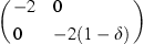 , whose leading coefficient is negative and whose determinant 4(1−δ) is positive as we assumed δ<1. Thus, the Hessian is negative definite and the profit function is strictly concave in (d
n
, d
r
). The associated Lagrangean is
, whose leading coefficient is negative and whose determinant 4(1−δ) is positive as we assumed δ<1. Thus, the Hessian is negative definite and the profit function is strictly concave in (d
n
, d
r
). The associated Lagrangean is 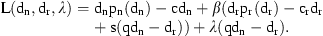
 satisfy the Kuhn–Tucker conditions
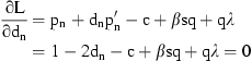
 and
and  .
.
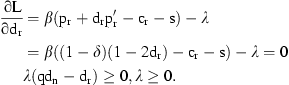
Case i: Assume that  . Then
  . From (A1), we obtain
  ; and from (A2), we obtain
 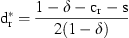 . We now need to check whether
  holds. Substituting and simplifying, we find that this condition holds if c
r
+s>(1−δ) (1−q(1−c+βsq)). If c
r
+s=(1−δ)(1−q(1−c+βsq)), then
holds. Substituting and simplifying, we find that this condition holds if c
r
+s>(1−δ) (1−q(1−c+βsq)). If c
r
+s=(1−δ)(1−q(1−c+βsq)), then  and
and  .
.
Case ii: If c
r
+s<(1−δ)(1−q(1−c+βsq)), then  cannot be 0;
  must hold. In this case,
  . To solve for
  , solve for λ in (A2) and plug it into (A1):
  . Then
  . To check that
  , we substitute
  into (A1), which yields the condition c
r
+s<(1−δ)(1−q (1−c+βsq)). This is what we had assumed, so we are done. □
into (A1), which yields the condition c
r
+s<(1−δ)(1−q (1−c+βsq)). This is what we had assumed, so we are done. □
Proof of Lemma 2. The maximum profit in period 1 is 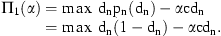
 . The corresponding price is
 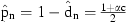 and the corresponding profit is
 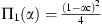 .
.
The maximum profit in period 2 is 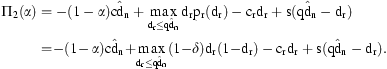
 is concave unimodal and attains its maximum at
  . Therefore,
 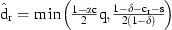 . Note that
 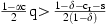 if and only if c
r
+s>(1−δ)(1−q(1−αc)), or, written in terms of α,
if and only if c
r
+s>(1−δ)(1−q(1−αc)), or, written in terms of α, 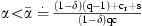 . That is,
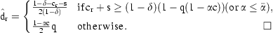
Proof of Proposition 1. Let Π(α) be the discounted total profit of the firm as a function of α. Then 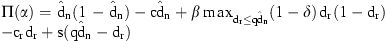 . Now let's calculate Π(α) under the two cases we identified.
Case (a): c
r
+s≥(1−δ)(1−q(1−αc)). In this case, Π(α) has the form −c
2
α
2/4+(c
2−βsqc)α/2+C, call it Π
a
(α). This function is concave unimodal and the point that satisfies the first‐order condition is  .
.
Case (b): c
r
+s<(1−δ)(1−q(1−αc)). In this case, the profit function, denoted by Π
b
(α), is again concave unimodal and the point that satisfies the first‐order condition is 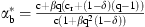 .
.
We can write  . We find that
 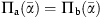 and
and 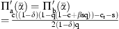 . Therefore,
  is a continuous function and
  if
if  , with
  otherwise. Note that
 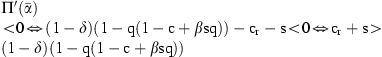 . This is the same condition as in the optimal firm‐wide analysis. We conclude that the threshold level where d
n
becomes a constraint for d
r
is the same as under the firm‐wide optimal analysis, which is the desired outcome.
. This is the same condition as in the optimal firm‐wide analysis. We conclude that the threshold level where d
n
becomes a constraint for d
r
is the same as under the firm‐wide optimal analysis, which is the desired outcome.
If c
r
+s≥(1−δ)(1−q(1−c+βsq)), we need to substitute  in
in  . We find
 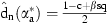 .
.
If c
r
+s<(1−δ)(1−q(1−c+βsq)), we need to substitute  in
in  . We find
 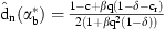 . □
. □
Proof of Proposition 2.  for any d
n
. We also need to determine
for any d
n
. We also need to determine  . At the firm‐wide optimal solution, the marginal cost to the firm equals the marginal revenue of the firm:
  . In case (i),
  and
and  , yielding
  . In case (ii),
  and
and 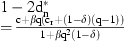 , yielding
 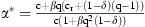 . □
. □
Proof of Corollary 1. For a given d
n
, the optimization problem of the firm and of the remanufacturing division is identical in our model: to choose d
r
so as to maximize (p
r
(d
r
)−c
r
)d
r
+s(qd
n
−d
r
) subject to the constraint d
r
≤qd
n
; there is no misalignment of incentives between the remanufacturing division and the firm. The remanufacturing division underproduces relative to the centralized benchmark ( ) only if it is constrained to do so by the manufacturing division's decision. Once the manufacturing division's incentives are aligned with those of the firm, the remanufacturing division naturally chooses
  . Now consider a cost allocation scheme that allocates an arbitrary function f(d
r
) to the remanufacturing division such that this division maximizes f(d
r
)+(p
r
(d
r
)−c
r
)d
r
+s(qd
n
−d
r
) subject to the constraint d
r
≤qd
n
. Unless f′(d
r
)=0, the first‐order condition of the remanufacturing division will differ from that of the firm, introducing a misalignment of the divisional objective with that of the firm. Therefore, the only cost allocation mechanism that will work is to have f(d
r
) be a constant independent of d
r
. □
. Now consider a cost allocation scheme that allocates an arbitrary function f(d
r
) to the remanufacturing division such that this division maximizes f(d
r
)+(p
r
(d
r
)−c
r
)d
r
+s(qd
n
−d
r
) subject to the constraint d
r
≤qd
n
. Unless f′(d
r
)=0, the first‐order condition of the remanufacturing division will differ from that of the firm, introducing a misalignment of the divisional objective with that of the firm. Therefore, the only cost allocation mechanism that will work is to have f(d
r
) be a constant independent of d
r
. □
Footnotes
Acknowledgments
The authors would like to thank Vishal Agrawal for setting up the numerical study, and Atalay Atasu, Daniel Guide, Luk Van Wassenhove, the associate editor, and two reviewers for comments that significantly improved this paper. This work was originally conducted when both authors were affiliated with INSEAD.
1We thank Luk Van Wassenhove for bringing the first two examples to our attention.
2This result holds with negative salvage value or with a disposal cost charged to the remanufacturing division. With a disposal cost v charged to the manufacturing division, if c r +s≥(1−q(1−c+β(sq−v(1−q)))(1−δ) and otherwise.