
Abstract
We develop a model that captures dynamic relationships of a supply chain populated by a dominant retailer and a number of fringe retailers. The two types of retailers are asymmetric in buying power, retailing cost, and the ability to service the manufacturer's product. The wholesale prices offered through a quantity discount (QD) schedule can coordinate such a supply chain, but invite channel flow diversion type of gray trading between the dominant retailer and the fringe retailers. Our analysis is focused on how such a channel can be coordinated and the gray market activities be prevented. We propose a dynamic QD contract or a revenue‐sharing contract that the manufacturer can use to fight the gray market activity. The performance of the supply chain and the manufacturer's profit under each of the two contract forms are compared and managerial guidelines are provided to help the manufacturer make a judicious choice.
1. Introduction
Today, the proliferation of distribution channels has presented manufacturers with unprecedented opportunities to bring their products to market. For instance, professional skin care manufacturers can distribute their products through a variety of channels, including department stores, drugstores, specialty retailers such as salons and wellness centers, skin care professionals such as dermatologists and plastic surgeons, and direct sales through infomercials, catalogs, and websites. However, manufacturers are being challenged more than ever when managing such a diverse distribution network. When a manufacturer sells to a certain mail‐order distributor, a contractual clause usually states that they cannot sell the product over the counter. However, it is not rare for mail‐order products to end up online somewhere, or being sold on the shelves of local drugstores. Although products ranging from skin care and beauty, pharmaceuticals, IT, and electronics are the frequently reported victims of this practice, just about every product sold, from cars to crackers, can be diverted from their intended channels. Diversion is a big business, with annual sales in the United States in the tens of billions of dollars. The largest diverter, Quality King Distribution of Long Island, does more than US$2 billion a year in business. It made news in 1998 when it appealed to the Supreme Court and won a copyright case involving diverted hair products (Bandler and Burke 2009). Diversions like this are not necessarily illegal per se. The term diversion simply refers to a situation where distribution channels somehow evade a manufacturer's control and merchandise is shifted from the intended distribution channel. It is a type of gray market called “channel flow diversion” or “product diversion.”
The most benign form of diversion serves free market objectives—when there is an oversupply of goods in one geographic location and paucity in another, by providing equilibrium. More often, however, it is price, not availability, which drives the diversion market. Uneven transfer/wholesale prices are often observed in a distribution network where one or a few power retailers dominate due to two reasons. First, the size of dominant retailers and the resulting buyer power allows them to obtain more favorable trade terms from manufacturers. Their ability to boost demand via advertisements and servicing manufacturers' products also signals a shift of profit away from the manufacturer. However, competing retailers of the dominant player in the same market do not enjoy the same kind of leverage with the manufacturers. For example, a group of more than 100 auto parts retailers claimed that category killers, including Walmart and Pep Boys, purchased auto parts from the suppliers at prices 40% less than the other retailers (Balto 2002). Second, from the manufacturer's perspective, potential benefits usually arise when working with dominant retailers due to dominant retailer's sheer size and the velocity at which they push product to market. Trade promotions, quantity discounts (QDs), rebates, chargebacks, and co‐op credits are the usual pricing means for a manufacturer to favor dominant retailers. However, the resulting price differentials contain rich incentives for channel flow diversion. In 2004, HP filed suit in a Tennessee federal court to recover more than US$8.6 million in pricing discounts for computer equipment that defendants falsely claimed were purchased by Capital City Micro Inc. of Tennessee for resale to P&E Distributing of Kentucky. HP's complaint sets forth claims for damages that include civil conspiracy and breach of contract. Although channel flow diversion is ubiquitous, high value products such as some industrial goods where manufacturers usually offer as much as 50% off ticket price are most susceptible to diversion. One of the authors of this paper worked for a company that designed and produced industrial automation control devices in Mainland China. At one time, the company had 36 distributors nationwide. Big distributors were given a deeply discounted price due to their large sales volumes. A few years into the implementation of the QD policy, the company saw a significant shrinkage in the number of distributors, even though the annual sales kept the momentum of healthy growth. On investigation, it was found that the majority of the “nonactive” distributors were actually still carrying the company's products, but they are getting their supply from big regional distributors, instead of from the company directly. No doubt the company's average profit margin suffered because the noncompliant distributors were costing the company millions in unwarranted and unearned discounts, and at the same time the company lost the opportunity to use price discrimination on those small distributors.
Channel flow diversion costs companies worldwide tens of billions of dollars a year in lost revenue. It is widespread, and, to the consternation of executives, often legal (Datz 2005). Many manufacturers already feel the pinch, and are hiring consulting firms to fight diversion. The usual practices adopted are in‐depth audits and a continuing monitoring of operations such as associating serial numbers, product master data, and distribution channel information for the life of the product, and allowing trusted parties to access product identification, location, status, and event data at any point in the supply chain. Coded package labeling is also a necessity. These practices deter diversion activities to some extent. However, a few major drawbacks limit the success. First, the world of diversion has become high tech, online, and extremely sophisticated. It is very costly for manufacturers to effectively trace products throughout the supply chain, and for the entire lifecycle of the product. The majority of manufacturers do not even have the resources or expertise to run such a sophisticated information system. Second, product tracking and tracing is only economical when applied at bulk size (except for high value items), and diverters usually break bulk and repackage products. Third, the diverters are very often legitimate partners or an employee within the manufacturing and distribution processes and therefore the resolution usually requires the highest level of discretion. Putting a business partner on notice that it will be subject to an audit is a difficult step for manufacturers in any industry. Some manufacturers see it as contrary to building and developing a cooperative business relationship.
The motivation of this research is to provide a solution that touches the essence of the issue: to design contracts that can manage the asymmetric relationships in the distribution network by aligning different wholesale prices in the price harmonization zone. We focus on two most popular contract types in distribution: QD and revenue sharing. We show how the two types of contracts can be applied in managing a distribution network where retailers have asymmetric buying powers and retailing costs. The effectiveness of each contract type in deterring/preventing channel flow diversion are discussed and compared. To the best of our knowledge, this is the first paper that addresses the issue of channel coordination in the context of channel flow diversion type of gray market activities.
The remainder of the paper is organized as follows. Section 2 surveys the related literature. Section 3 presents our model and derives a QD schedule that coordinate a decentralized channel. Section 4 shows how retailers can profit from channel flow diversion and the impact of it on the manufacturer. Section 5 derives a dynamic QD schedule and a revenue‐sharing contract to fight gray market, and compares the two contract types. Concluding remarks are made in section 6.
2. Related Literature
This research is mainly in the nexus of three streams of literature: the literature on channel coordination, the literature on channel structure with asymmetric relationships, and the literature on gray market. We now discuss how this paper borrows from and contributes to these streams.
In the channel coordination literature, Jeuland and Shugan (1983) showed that channel coordination can be obtained using QD. Moorthy (1987) showed that optimal price that can maximize channel profit can be obtained using a two‐part tariff. This type of two‐part tariff can coordinate a channel where the retailer provides the value‐added service (Lal 1990). Weng (1995) examines the effect of QDs from an operations management perspective. Gan et al. (2004) found that a revenue‐sharing contract can achieve a Pareto‐optimal joint action in which a less risk‐averse agent assumes more risk by taking a larger portion of the channel's random profit. The agents' final payoffs can be adjusted by a side payment depending on their respective bargaining powers. In a dynamic model, He et al. (2009) found that a revenue sharing and co‐op advertising contract where the manufacturer receives a constant fraction of the retail revenue and contributes the same fraction toward co‐op advertising will coordinate the channel. We build on this stream of literature by considering the potential effects from implementing these contracts, and adapt contract terms to fight channel flow diversion. A few studies (see, e.g., Blair and Lewis 1994, Desai and Srinivasan 1995, Desiraju and Moorthy 1997,Mukhopadhyay et al. 2008, 2009) investigate contract design in the presence of retailers' marketing/value‐adding efforts. Our research complements these studies and provides new insights for helping a manufacturer to make a judicious choice between two contract types under different conditions.
In the literature on channel structure with asymmetric relationships, Raju and Zhang (2005) examine the manufacturer's channel coordination policies in the presence of a dominant retailer. Our research is closely related to theirs, but our focus is on fighting channel flow diversion, with channel coordination as a secondary concern. In a similar setting, Cui et al. (2008) show that the manufacturer can use trade promotions to price discriminate between the dominant retailer and smaller independents because trade promotions induce different inventory‐ordering behaviors. Dukes et al. (2006) find that the manufacturer can increase its profit based on a bilateral bargaining which transfers market share to the more efficient retailer. Geylani et al. (2007) examines a manufacturer's strategy in response to a dominant retailer who has the power to dictate the wholesale price and concludes that the manufacturer should transfer demand to the weak retailer by engaging in joint promotions and advertising. Chen (2003) demonstrates that an increase in the amount of countervailing power possessed by a dominant retailer can lead to a fall in retail prices for consumers, while total surplus does not always increase accordingly. Lau et al. (2007) examine a channel where the dominant retailer has imperfect knowledge of the manufacturer's production cost. The authors derive optimal decision approaches for the dominant retailer when he has to choose between a retailer–Stackelberg and a manufacturer–Stackelberg game. In contrast to the above research that emphasizes various tactics a manufacturer/dominant retailer can use to maximize a particular party's surplus, our paper enriches the literature by focusing on creating harmonization across the network, which we believe is more sustainable.
The literature on gray market can be divided into two broad categories. The first category (see, e.g., Antia et al. 2004, Dana 1998, Danzon 1997, Kuhn 1998, Michael 1998, Vickers 1997) focuses on general discussions over causes and remedies of gray market activity from the practitioners' point of view. This category of literature is enriched by a number of industry news from trade journals discussing the current practices in gray market activity. Alliance for Gray Market and Counterfeit Abatement (AGMA) website,
The second category focuses on theoretical analysis and empirical verification of gray market activity and manufacturers' strategies. Yang et al. (1998) and Ahmadi and Yang (2000) provide theoretical support that a firm can use pricing strategies to increase sales volume and growth when facing gray market activity. Unlike their paper, our research focuses on the most deceptive form of gray market; the type that is initiated by legitimate distributors already in the network (rather than by consumers or brokers). Hence, our conclusion is different from theirs, and shows that it is always in the manufacturer's best interest to deter/contain channel flow diversion type of gray market. Gerstner and Holthausen (1986) analyze profitable pricing when market segments overlap. Overlapping markets are segments that are not perfectly sealed, and leakage between them can occur. They conclude that when the price differentiation is optimal, the equilibrium amount of leakage is determined endogenously. They also show that price differentiation can be optimal even when leakage between markets is substantial. Bergen et al. (1998) propose that tolerance of gray market activity is a function of a firm's ability to detect violations, and of the existence of credible threats and commitments. Chintagunta and Desiraju (2005) empirically show that the interfirm strategic interactions both within the market and across markets makes observed prices more similar across countries than prices implied by estimated elasticity. Our paper complements the aforementioned research because we confirm that harmonizing prices and/or accepting a certain level of leakage can be good solutions under certain conditions although we derive the results from quite different models.
3. The Model
We consider a distribution channel consisting of a manufacturer selling through one dominant retailer and N other retailers (we call them “fringe retailers” hereafter). Following the lead by Raju and Zhang (2005), we assume that the dominant retailer has market power and faces a downward‐sloping demand curve given by 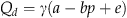
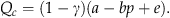
The total sales by the manufacturer is the total of (1) and (2)
3.1. The Integrated Supply Chain
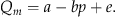
In this subsection, we study the integrated model where the manufacturer, the dominant retailer, and the fringe retailers effectively act as a single firm. The manufacturer acts as a central planner, and sets the market price (p), and service (e) directly. The manufacturer incurs a constant marginal production cost (c), and retailers incur a retailing cost. Without loss of generality, we assume that the dominant retailer's unit retailing cost is zero, and the fringe retailers incur a unit retailing cost (s), where s>0, implying that the fringe retailers are not as efficient as the dominant retailer in retailing. Intuitively, the solution to this integrated model will provide the first best solution and can be used as a baseline for our subsequent analysis. The manufacturer solves the following optimization problem: 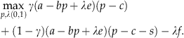
We have the optimal price, sales, and resulting channel profit as 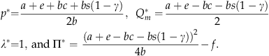
Here, we need the assumption that the service cost f is limited by the upper boundary 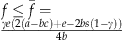 , when this is satisfied, the service is ensured.
3.2. Decentralized Supply Chain with Independent Retailers
In case of a decentralized supply chain, a Stackelberg game is played where the manufacturer is the leader. The dominant retailer needs to decide on the optimal values of retail price p, and whether or not to provide service in response to the manufacturer's decision variable w, the wholesale price. The dominant retailer's profit function is 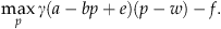
Maximizing this, we obtain the dominant retailer's response function as 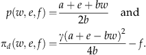
The dominant retailer will provide service only if π
d
(w, e, f )≥π
d
(w, 0, 0), or 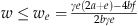 . Anticipating the dominant retailer's response, the manufacturer decides whether to motivate the retailer to provide service or not. Each party's decisions at equilibrium are summarized in Table 1, and Figure 1 uses numerical examples to illustrate these results.

 .
.
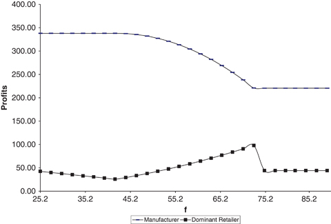
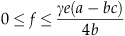
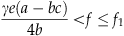
As shown in Figure 1, in a noncoordinated supply chain, the manufacturer's profit is nonincreasing in f. When 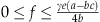 , the dominant retailer would provide service unconditionally. In that case, the manufacturer's profit does not vary with f and the dominant retailer's profit decreases with f. As f increases further, i.e.,
 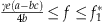 , the dominant retailer will not provide service unless the manufacturer lowers the wholesale price accordingly to make it profitable to service the product. Because of the lowered wholesale price, the manufacturer's profit decreases as f increases. On the other hand, the reduction in the wholesale price more than offsets the increase in the service cost incurred by the dominant retailer. As a result, the dominant retailer's profit even increases as f increases. When f increases beyond
  , it is too costly for the manufacturer to motivate the retailer for service provisions. In that case, no service is provided. In such a non‐coordinated supply chain, the maximum channel profit cannot be achieved because the classic double marginalization problem causes the retail price to be too high and service provisions distorted. Note also that neither the manufacturer nor the dominant retailer considers the retailing cost incurred by the competitive fringe while making their pricing decisions. Recall from Equation (5) that, in a coordinated supply chain, the discrepancy in retailing efficiency between the dominant retailer and the competitive fringe is reflected in the retail price.
3.3. Use of Pricing Mechanism to Achieve Channel Coordination
In section 3.2, we have a noncoordinated supply chain that does not achieve the maximum supply chain profit due to double marginalization. The manufacturer can bring the dominant retailer's interests in line with the supply chain's interests using a suitable pricing mechanism. For this purpose, we propose a QD schedule as given in Jeuland and Shugan (1983). With QD, a wholesale price will decrease as order volume increases. Moreover, a subsidy may also be provided for the service provided by the dominant retailer. The intuition is, if the dominant retailer is offered a lower wholesale price, she in turn would set a lower retail price that can maximize the supply chain's profit.
The wholesale price that each retailer faces is thus a function of q and f, namely w(q, f ). Note that f=0 for all fringe retailers. The dominant retailer's profit function is 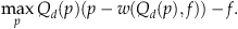
A mechanism for aligning the dominant retailer's profit with the supply chain's profit can be devised by transforming Equation (8) into 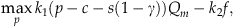
P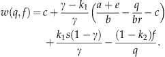
We can determine the values of k
1 and k
2 if we assume that the manufacturer uses just the minimum level of incentives to induce the dominant retailer to service her product, while keeping the fringe retailers in the market. The optimum values of k
1and k
2 are as follows: 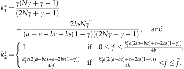
Substituting these into Equation (10), we obtain the optimal discount schedule that coordinates the channel as 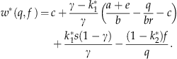
Looking at Equation (12), we see that the larger the order size, the lower is the unit wholesale price. Because  , the dominant retailer is offered a lower wholesale price than fringe retailers (w
d
<w
c
). The incurred service cost, if any, further reduces her wholesale price. Fringe retailers are left with zero profit because k
1 and k
2 are determined in such a way that the product's retail price equals the total of the wholesale price to the fringe retailers and their unit retailing cost. Both the manufacturer and the dominant retailer are better off in the coordinated supply chain, not only because the maximum channel profit is achieved, but also because the QD schedule extracts all profit from the competitive fringe. In other words, the channel profit is exclusively distributed between the manufacturer and the dominant retailer. Figure 2 depicts how each party's profit varies with the service cost ( f ) under the QD schedule.
, the dominant retailer is offered a lower wholesale price than fringe retailers (w
d
<w
c
). The incurred service cost, if any, further reduces her wholesale price. Fringe retailers are left with zero profit because k
1 and k
2 are determined in such a way that the product's retail price equals the total of the wholesale price to the fringe retailers and their unit retailing cost. Both the manufacturer and the dominant retailer are better off in the coordinated supply chain, not only because the maximum channel profit is achieved, but also because the QD schedule extracts all profit from the competitive fringe. In other words, the channel profit is exclusively distributed between the manufacturer and the dominant retailer. Figure 2 depicts how each party's profit varies with the service cost ( f ) under the QD schedule.
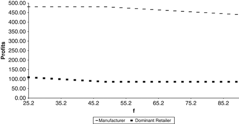
Figure 2 shows that both parties' profits are non‐increasing in service cost ( f ), which reflects the fact that the two parties' interests are aligned by the QD schedule. It is worth mentioning that, in the QD schedule, retailing cost s, incurred by the fringe retailers, is treated as a built‐in cost of the supply chain, just as the way c is treated. One might think that the fringe retailers play no role in channel coordination because they are price followers, and as a result, it would be sufficient for the manufacturer to coordinate the pricing decisions with the dominant retailer. One intuitive explanation of the inclusion of s in the wholesale price schedule is as follows. Since the retailers in the competitive fringe account for 1−γ of the total market sales, their retailing cost is part of the supply chain cost, and it should be reflected somewhere. In addition, in order not to price the fringe retailers out of the market, it is necessary to include the retailing cost (s) in the wholesale price schedule up front, preventing the case where the dominant retailer would settle for a retail price that is too low to cover the fringe retailers' retailing cost. Recall that, when the channel is not coordinated, neither the wholesale price (determined by the manufacturer) nor the retail price (determined by the dominant retailer) reflects the retailing cost incurred by the fringe retailers. It only reminds us that, in a noncoordinated supply chain, fringe retailers earn a strictly positive profit because of the high retail price.
4. Gray Market Activity
Because of the different wholesale prices offered through the QD schedule, the dominant retailer has a great incentive to purchase more than her own needs, and resell the extra to the fringe retailers at a price somewhere between the two wholesale prices. Many evidences are seen in real life. Kimberly–Clark, maker of well‐known brands such as Huggies and Kleenex, once found that one of their major distributors had been purchasing secondary product—product coming from secondary dealers (Datz 2005). When asked for an explanation, the distributor said they are a business, and it is a business decision (secondary dealers offered lower prices than the manufacturer). Anecdotal evidence of gray market problems became stronger at Xerox in 2006. They began a program that manually marked goods prior to shipment, and marked goods were later found coming back into nonauthorized regions. Subsequent analysis of partner volume needs revealed an over‐shipment of more than 30%, which proved the existence of channel flow diversion. Because the manufacturer does not authorize the transaction between the dominant retailer and the fringe retailers, which is in a realm between legitimate market and black market, it is called gray market. It is a situation where distribution channels evade the manufacturer's control, and hence we label it as “channel flow diversion” type of gray market. In this section, we quantitatively evaluate the impact of channel flow diversion.
In practice, the QD contract usually applies to accumulative sales occurred in a selling season of one year or a quarter year. During the selling season, retailers may order a few times, and the transfer prices can be different from the QD price that a retailer is entitled to. At the end of the selling season, there will be a lump sum adjustment based on the actual sales between the manufacturer and the retailers according to the QD schedule. Even if the manufacturer observes unusually large orders from the dominant retailer during the selling season and fewer number of orders from fringe retailers, the manufacturer cannot be conclusive about what is going on. Besides, the manufacturer cannot make a unilateral change in the QD that he has committed to before the selling season. As such, we call the QD schedule provided in Equation (12) as a fixed QD schedule. Let n<N be the number of fringe retailers that join the dominant retailer in a gray market alliance. The dominant retailer represents the alliance and orders  . The alliance is entitled to a lower wholesale price
 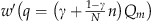 because of the higher order quantity. Obviously, there is a shift of profit from the manufacturer to the alliance. The profit for the alliance is
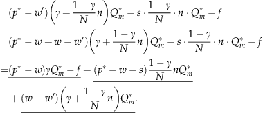
Note that w is the wholesale price that the dominant retailer is entitled to without gray market, and w′ is the lower wholesale price that the alliance is entitled to due to the aggregated order size. Equation (13) shows that the alliance's profit consists of three parts: the first part is the dominant retailer's guaranteed profit regardless of the existence of a gray market; the second part shows that the fringe retailers who joined the alliance can be at least entitled to the same wholesale price t that the dominant retailer has had, and as a result, they earn a positive profit now; the third part is the additional profit that the alliance has earned because of the lowered wholesale price. Note that the total additional profit because of the gray market is the sum of part two and part three, and the dominant retailer and the fringe retailers can arbitrarily divide it among them. Let G be the gray market profit, then 
P
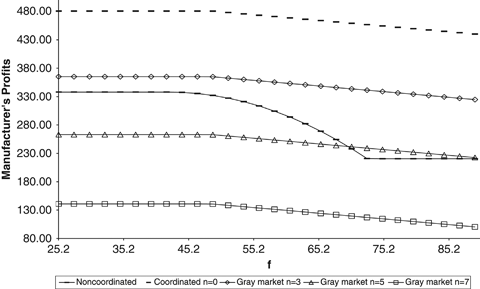
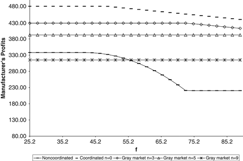
Figure 3 depicts the manufacturer's profit under dynamic QD schedule with different gray market size, measured by the number of fringe retailers involved in gray market, and compares it with that of a non‐coordinated supply chain. It shows that the manufacturer achieves the highest profit under the QD schedule if no gray market exists. The manufacturer's profit decreases as the number of fringe retailers involved in gray market increases. When the size of gray market is considerably large, the manufacturer does not benefit from offering the QD schedule any more. For example, when seven out of 10 fringe retailers choose the gray market, the manufacturer's profit is lower than that of a noncoordinated supply chain for all values of f.
5. Fighting Gray Market
In this section, we explore various options for the manufacturer to fight gray market. First, we consider the possibility that a QD schedule and channel coordination can be sustained simultaneously in presence of gray market threat. To eliminate gray market activities, the manufacturer needs to ensure that the gray market profit derived from cheating is no more than what the fringe retailers can get if they directly trade with the manufacturer.
Let k″1 and k″2 be the parameters of the QD schedule, which guarantees the fringe retailers a unit profit of δ if they directly trade with the manufacturer. Given the QD schedule, if n fringe retailers decide to participate in gray trading with the dominant retailer, the profit for the alliance becomes 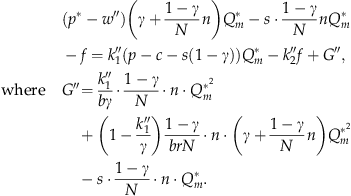
To eliminate gray market activities, the manufacturer needs to equate the following: 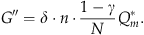
The resulting equilibrium points are k″1=γ and k″2=1. Substituting k″1=γ and k″2=1 back into discount schedule (10), we have a wholesale price for both types of retailers as W
d
=w
c
=c+s(1−γ), which is no longer a discount schedule. Therefore, it is not possible to eliminate gray trading within the framework of a QD schedule. The resulting profits for each party are 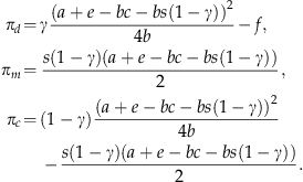
Even though the channel is coordinated, the manufacturer is left with low profit. If the competitive fringe is equally efficient in retailing as the dominant retailer, i.e., s=0, the manufacturer will make zero profit.
5.1. Dynamic QD Schedule
After observing gray market activities, the manufacturer can always threaten to terminate the contract with the dominant retailer, but such a threat may not be viable. Intervention with economic means is usually more effective. Here we propose an alternative discount schedule called the dynamic QD schedule. In this schedule, the manufacturer reserves the right to conduct channel audit and adjust k
1 and k
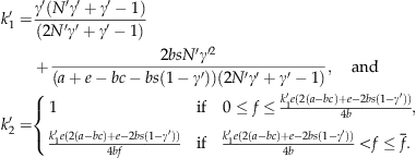
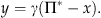
2 based on the observed γ and N. After one selling season, the manufacturer would observe the updated market share 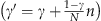 and the number of fringe retailers that purchase from the manufacturer directly (N′=N−n), and accordingly, the manufacturer would adjust QD parameters to k′1 and k′2. The dynamic QD schedule is given by
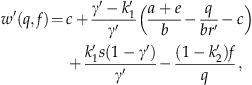
It is worth pointing out that Equation (18) transforms the dominant retailer's problem as follows: 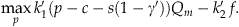
Since the supply chain profit is (p−c−s(1−γ))Q m −f, Equation (20) is no longer an affine transformation of the supply chain profit equation. The retailing cost of the fringe retailers who are involved in gray market is not presented in Equation (20), because that part of supply chain evades the manufacturer's control. We name that cost as “gray market retailing cost.” Hence, k′1 is the fraction of total channel profit, excluding the service cost, and excluding gray market retailing cost, that the alliance can capture. The parameter k′2 is the fraction of service cost that the dominant retailer cannot recover. It can be proved that k′1 is increasing in n, while k′2 is nondecreasing in n. As n increases, the increase in k′1 will increase the alliance's share of channel profit, however, the non‐decreasing value of k′1 will erode its profit. The balancing effect of k′1 and k′2 protect the manufacturer from severe loss due to excessive gray market activities. Recall that the gray market retailing cost is solely shouldered by the alliance, which further suppresses the shift of profit from the manufacturer to the alliance.
Since Equation (20) is not an affine transformation of the supply chain profit function, we expect that channel coordination cannot be achieved. Proposition 3 summarizes the supply chain performance under the dynamic QD schedule.
P compared with the optimal profit of a coordinated supply chain. The dominant retailer's optimal retail price will decrease as the number of fringe retailers that participate in gray market increases, and specifically,
 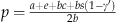 .
.
Because  is a small number, the supply chain profit under the dynamic QD schedule is not much different from that of a coordinated supply chain even with excessive gray market activities. Now, let us examine the manufacturer's profit under the dynamic QD schedule
Because of the piecewise nature of k′2 and the continuous adjustment of k′1 based on n, the variation of π m with respect to n cannot be proved analytically. However, extensive numerical studies carried out by us show that the manufacturer's profit always decreases as n increases.
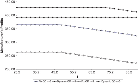
Figure 4 depicts the manufacturer's profit under the dynamic QD schedule with different gray market size, and compares it with that of a noncoordinated supply chain. Resembling the case of a fixed QD schedule, Figure 4 verifies that the manufacturer's profit achieves the highest level under the dynamic QD schedule if no gray market exists and it decreases as gray market size (n) increases. However, the dynamic QD schedule makes the manufacturer less vulnerable to the gray market activity, which is clearly seen from the significantly improved profits. For instance, if all other conditions are held constant, when five out of ten retailers are involved in gray market, the manufacturer would discard fixed QD schedule if f is not extremely high (as shown in Figure 3). But Figure 4 shows that, for a wide range of f that falls toward the higher end of the continuum, the manufacturer still benefits even when nine out of 10 retailers are involved in gray market. Figure 5 shows that, for the same level of gray market activity, the manufacturer's profit is higher under the dynamic QD schedule, compared with the fixed QD schedule.
Note that the above result is conditioned on n<N. Obviously, all retailers have incentive to join the dominant retailer in the alliance. However, the dominant retailer would not choose to ally itself with all of them because of the fact that the manufacturer could aggressively lower k′1 if there is no need to worry that retailers in the competitive fringe might be priced out of the market.
5.2. Revenue‐Sharing Contracts
It is widely known that revenue‐sharing contracts coordinate a vertical channel with a manufacturer and a retailer. However, it has not been explored if it can effectively contain gray market activities in a supply chain with asymmetric retailers. With a revenue‐sharing contract, a retailer pays the manufacturer a wholesale price for each unit purchased plus a percentage of the revenue the retailer generates. Under revenue sharing, the manufacturer must monitor the retailers' revenue to verify that they are split appropriately. Usually, a point of sales system at the retailer's end, which allows the manufacturer an access through extended intranet or EDI, would serve the purpose. However, the gains from coordination may not always cover the costs of this infrastructure, which may partially explain why revenue sharing is not implemented in some settings. Despite this disadvantage, revenue‐sharing contracts are extremely popular among supply chain participants who seek relational exchanges and focus on profit in the long run.
Before the dominant retailer determines retail price and decides whether to provide service, the manufacturer and the dominant retailer agree to a revenue‐sharing contract, which generally consists of two parameters: the wholesale price (w d ) the dominant retailer pays per unit and the dominant retailer's share of revenue (φ d ). Let the revenue‐sharing contract with the fringe retailers be denoted by {w c , φ c }.
The profit functions for the dominant retailer, the fringe retailers, and the manufacturer are, respectively, 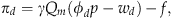

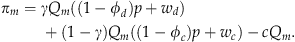
The channel can be coordinated if  maximizes π
d
. In other words, the revenue‐sharing contract achieves supply chain coordination by making the dominant retailer's profit function an affine transformation of the supply chain's profit function.
maximizes π
d
. In other words, the revenue‐sharing contract achieves supply chain coordination by making the dominant retailer's profit function an affine transformation of the supply chain's profit function.
P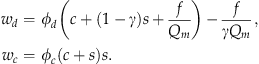
The resultant respective profits are


Proposition 4 can be verified by substituting w
d
into Equation (22) to obtain Equation (25). Equation (25) states that the dominant retailer captures a portion (γφ
d
) of the total supply chain profit, whereby the retailer's profit is aligned with the supply chain's. The dominant retailer is motivated to provide service and set the market price as that of an integrated channel  . Equation (26) states that φ
c
portion of the profit realized through the competitive fringe goes to the competitive fringe. The exact value of φ
d
(φ
c
) can be determined mutually between the manufacturer and the dominant retailer (the competitive fringe) depending on their relative negotiation power. However, the manufacturer would avoid φ
c
=0 even if it has the absolute power of doing so. If φ
c
=0, the fringe retailers would collude with the dominant retailer as long as they can obtain a positive profit from the collusion. Likewise, the dominant retailer has incentive to overstate its market share (γ) by colluding with the competitive fringe since its profit increases with γ. To avoid the gray market, the manufacturer will ensure that no party can benefit from the collusion. The maximum gray market profit possible through collusion with the dominant retailer is
. Equation (26) states that φ
c
portion of the profit realized through the competitive fringe goes to the competitive fringe. The exact value of φ
d
(φ
c
) can be determined mutually between the manufacturer and the dominant retailer (the competitive fringe) depending on their relative negotiation power. However, the manufacturer would avoid φ
c
=0 even if it has the absolute power of doing so. If φ
c
=0, the fringe retailers would collude with the dominant retailer as long as they can obtain a positive profit from the collusion. Likewise, the dominant retailer has incentive to overstate its market share (γ) by colluding with the competitive fringe since its profit increases with γ. To avoid the gray market, the manufacturer will ensure that no party can benefit from the collusion. The maximum gray market profit possible through collusion with the dominant retailer is 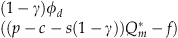 .
.
Let 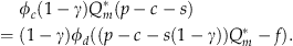
By this arrangement, neither the dominant retailer nor the competitive fringe has incentive to engage in gray trading, since no profit would be shifted from the manufacturer to the gray market. From (27), we have 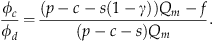
From Equations (27) and (28), we can derive the following proposition.
P
5.3. The Manufacturer's Choice
In this section, we compare the revenue‐sharing contract with the dynamic QD schedule, the result of which will help the manufacturer make a judicious decision. Apparently, the revenue‐sharing contract is very flexible in the sense that supply chain profit can be arbitrarily allocated between the manufacturer and the retailers based on negotiation. To make a sensible comparison with the dynamic QD contract, we need to have a valid expectation on negotiation outcome. We are going to focus on the negotiation between the manufacturer and the dominant retailer only, since Proposition 5 already shows that the negotiation between the manufacturer and the dominant retailer (φ d ) uniquely determines how supply chain profit is distributed.
5.3.1. Nash Bargaining Solution
Let us call x the desired profit for the manufacturer, and y the desired profit for the dominant retailer. Rational agents will choose what is known as the Nash bargaining solution. Namely, they will seek to maximize |x−x
0| |y−y
0|, where x
0 and y
0 are the status quo profits (i.e., the profit obtained if one decides not to bargain with the other player). The product of the two excess profits is generally referred to as the Nash product. It is not surprising that neither party will accept a profit that is less than what each can get in a noncoordinated supply chain. Hence, we set x
0=π
m
, y
0=π
d
, where π
m
and π
d
are given in Table 1. We can rewrite the bargaining problem as following: 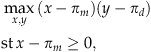

Note that Equation (31) is based on Proposition 5, and  is given in Equation (5). Solving the above problem, we have
P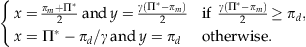
5.3.2. The Manufacturer's Profit
Note that the manufacturer's profit under revenue‐sharing contract is given in Proposition 6 and his profit under dynamic QD schedule is outlined in Equation (21). Because both are closed form solutions, by comparing the two profit levels, the manufacturer can make a judicious choice about the type of contract to be offered. However, the decision is not always clear‐cut due to the fact that the manufacturer is not sure about the gray market size, should a dynamic QD schedule be offered. Nevertheless, the manufacturer can still make a straightforward comparison that is contingent on gray market size. Although we can easily use the closed form analytical results to make the comparison, the mathematical expressions are too long to convey meaningful information. Rather, we choose to use numerical examples to illustrate the result qualitatively. Figure 6 plots the manufacturer's profit under revenue‐sharing contract and compares it with that under the dynamic QD contract when n=1, 5, 9 (out of N=10), respectively.
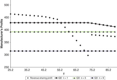
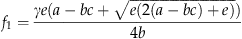
Figure 6 shows that the manufacturer's profit under revenue‐sharing contract is piecewise decreasing in f because of the constraint in Equation (30). Within certain range before the jump point, the manufacturer's profit decreases along a steep curve because the dominant retailer has a strong bargaining power. Because of the fact that the dominant retailer's bargaining power is determined by the profit she can get in a noncoordinated supply chain, comparing Figure 6 with Figure 1 and referring to Table 1, it is obvious that the segment of the steep curve before the jump point corresponds to the range of f, where the manufacturer has to cut wholesale price to stimulate the dominant retailer's service provision in a noncoordinated supply chain. As a result, the just point must be f 1 defined in Table 1.
Next, we define f n as the service cost at which the manufacturer's profit under revenue‐sharing contract equals that under dynamic QD contract when n fringe retailers participate in gray market (note that revenue‐sharing contract can proactively prevent gray market). Figure 6 shows that the manufacturer's profit is always higher under revenue‐sharing contract when 0≤f≤f 1; and is higher under dynamic QD contract when f n ≤f≤f 1, given that less than or equal to n fringe retailers participate in gray trading should dynamic QD contract be offered. f n and f 1 can be uniquely determined because of the closed form solutions derived in Proposition 6 and Equation (21). When f>f 1, the manufacturer's choice has to be investigated based on each individual case. In this numerical example shown by Figure 6, the manufacturer prefers dynamic QD contract when less than or equal to five fringe retailers are expected to participate in gray trading, and he prefers revenue‐sharing contract otherwise. Proposition 7 summarizes the manufacturer's choice.
P
When f n ≤f≤f 1, the manufacturer has to make a decision under uncertainty because, at the time the manufacturer decides on which contract type to offer, he is not sure how many fringe retailers will participate in gray trading if he offers dynamic QD contract. Still, the managerial guideline derived has important application in practice not only because it greatly simplifies the decision making, but also because, in reality, the manufacturer usually has a good estimate about n based on previous relationships with retailers and the ease with which to conduct channel audit. Other factors, such as a potential strategic distribution partnership on a new product line, and whether or not the manufacturer's threat of retaliation is viable, can be important inputs to the estimate as well.
6. Conclusions
In this paper, we have developed a model that captures dynamic relationships of a supply chain populated by a dominant retailer and a number of fringe retailers. The two types of retailers are asymmetric in buying power, retailing cost, and the ability to service the manufacturer's product and there is a danger of gray market activities developing. The focus of our analysis is primarily on how such a channel can be managed through aligning different wholesale prices in a harmonization zone so that gray market activities can be prevented.
We show that a QD schedule can coordinate such a channel. However, it gives the dominant retailer an opportunity to engage in gray market activities. Specifically, the dominant retailer could leverage its power to procure products at a big discount from the manufacturer and resell them to fringe retailers at a price lower than the wholesale price that the manufacturer offers to those fringe retailers. The result is a sizeable shift of channel profit from the manufacturer to retailers that are involved in gray trading. In view of this, we propose two types of contracts to counter this: a dynamic QD contract and a two‐part tariff‐based revenue‐sharing contract. The performance of each is discussed and managerial insights are derived to help the manufacturer make a judicious choice between the two contract types.
Specifically, a revenue‐sharing contract can prevent gray market and achieve channel coordination, whereas a dynamic QD contract always offers gray trading opportunity, and as a result, channel coordination cannot be achieved. However, a dynamic QD schedule can achieve a near optimal profit even with excessive gray market activities, which makes the total supply chain profit of lesser concern compared with the allocation of it. Generally speaking, if f is toward the lower end of the service cost continuum, i.e., 0≤f≤f 1, the manufacturer prefers a revenue‐sharing contract no matter what the gray market size would be (should a dynamic QD contract be offered). When service cost is in the middle, i.e., f n ≤f≤f 1, the dynamic QD contract is preferred if less than or equal to n fringe retailers are expected to participate in gray trading.
One interesting result is that a single linear pricing can also preclude gray trading and coordinate the channel. The manufacturer may earn a positive profit provided that the dominant retailer is more cost efficient in retailing. However, the manufacturer's profit is limited by the extent of cost asymmetry.
Our model is a first step in studying issues related to coordinating a channel with asymmetric relationships and asymmetric costs in the context of possible gray trading. Future research can relax some of our assumptions such as a fixed market share for the dominant retailer and identical fringe retailers. An alternative negotiation benchmark for the revenue‐sharing contract would lead to interesting results. It is also valuable to explore other contracts outside the frame of channel coordination to fight gray market.
Footnotes
Appendix
Acknowledgments
The authors are grateful to the senior editor and two anonymous referees for their valuable comments. Their suggestions have very much improved the paper. We also thank department editor Professor Suresh P. Sethi for his suggestions and help.