
Abstract
We examine the role of expediting in dealing with lead‐time uncertainties associated with global supply chains of “functional products” (high volume, low demand uncertainty goods). In our developed stylized model, a retailer sources from a supplier with uncertain lead‐time to meet his stable and known demand, and the supply lead‐time is composed of two random duration stages. At the completion time of the first stage, the retailer has the option to expedite a portion of the replenishment order via an alternative faster supply mode. We characterize the optimal expediting policy in terms of if and how much of the order to expedite and explore comparative statics on the optimal policy to better understand the effects of changes in the cost parameters and lead‐time properties. We also study how the expediting option affects the retailer's decisions on the replenishment order (time and size of order placement). We observe that with the expediting option the retailer places larger orders closer to the start of the selling season, thus having this option serve as a substitute for the safety lead‐time and allowing him to take increased advantages of economies of scale. Finally we extend the basic model by looking at correlated lead‐time stages and more than two random lead‐time stages.
Introduction
With products moving over longer distances and crossing more national borders and inspection points, the global supply chains of today are longer and more complex than the localized supply chains of the past. As a result, supply side risks have become a greater concern—particularly those that affect supply lead‐times. Operating in developing countries with low‐cost labor, but inadequate supply and production infrastructures, increases the potential for disruptions and unexpected delays. Exposed quality and yield problems due to lower worker skills and higher employee turnovers result in elongated production flow times. Furthermore, the transportation logistics components of the global supply chains are prone to serious and variable duration delays due to congested ocean ports, not only at the sourcing origins, such as the Shanghai port, but also at the destination ports, such as Long Beach, CA and Vancouver, Canada. Additionally, suppliers may not always see a need to offer short lead times (e.g., due to the “safety stock effect” studied in Kraiselburd et al. 2011).
The sourcing of goods from faraway locations, most recently from China and other Southeast Asia locations, are typically for higher volume stable demand products (“functional products” in the supply chain literature language, see Fisher 1997) in search of lower material and production costs. However, the efficiency of the flows in these longer chains, and consequently the “leanness” of them in terms of inventories, strongly relies on the predictability of these elongated lead‐times, which is far from the current state of affairs. Stalk (2006) warns supply chain managers of the hidden costs of elongated and variable lead‐time supply chains (e.g., the costs for stockouts, excess inventories and write‐downs, over‐ and under‐productions, etc.), and explicitly advises them to consider expediting options for effectively managing such chains. Such options, on the transportation logistics side, might go beyond air freight to paying premiums for preferred treatments from ground, sea, and air shippers, port services, and other suppliers. Crone (2006) reports on dynamic rerouting practices based on port congestion and other traffic bottlenecks. For example, a European food manufacturer supplies the North American market via shipments routing through the Montreal port instead of the heavily congested East Coast ports. On the production side typical expediting options might involve processing part of the order in an expedited way, possibly through extra shifts and overload pay. Throughout the article, our use of the term “expediting” implies shortening of lead‐time, in expectation, to reach the point of sale, and it covers any of the above‐mentioned production and logistics expediting alternatives. Other alternatives we view as expediting include point‐to‐point shipping via bypassing intermediate consolidation and distribution points, and preferential treatment services by supply and logistics intermediaries—such as “priority processing” and “unloading your goods first”—at extra payment.
From an implementation perspective, we are now more than ever capable of employing sophisticated expediting options. Advances in information technology have greatly facilitated information flows in supply chains. The emergence of new technologies such as radio frequency identification (RFID) further enables the visibility of a certain item along a supply chain. By collecting data contained in small tags attached on items, RFID efficiently tracks in real‐time where and when these items (product, case, or pallet) are (e.g., Gardner 2004, Wolfe et al. 2003). These technologies allow recording in detail the duration of the various stages in the product's journey from source to destination, thus accounting for the major sources of unpredictable variability in the product's production and logistics flow path. For example, readers may be installed at in‐ and out‐bound docks, loading and unloading points, custom inspection stations, ships, trucks, planes, and so on. As products pass through intermediate production and logistics points, the readers can identify them and broadcast this information immediately.
Motivated by our discussion above, in this study, we aim to examine the use of an expediting service and its implications in the cost of meeting demand, the planning of safety lead‐times, and order sizes for “functional goods.” To do so, we use a stylized single‐product demand model with a constant demand rate where the lead‐time of the replenishment orders is stochastic. The lead‐time consists of two stages with random duration. At the completion time of the first stage, the firm can decide whether to expedite some or all of the replenishment order. The expediting service has a deterministic lead‐time but is more expensive.
Our research clearly outlines the nature of the optimal expediting policy in terms of whether and how much to expedite: (i) when the expediting cost is too high (above a defined threshold in Proposition 1), it is optimal not to employ expediting; (ii) when the expediting cost is low (below a defined threshold in Proposition 2), it is optimal to fully exploit the expediting opportunity and use it aggressively; and (iii) when the expediting cost is intermediate (i.e., between the two defined thresholds), it is optimal to adopt the expediting service but only leverage it in a limited way. The optimal expediting policy formalizes some of our intuition, but it also offers insights that could be perceived as surprising to our “raw” intuition. Specifically, it shows that when a replenishment order has longer delays, it is not necessarily true that one would expedite a larger portion. The impact for factors such as the cost and lead‐time of the expediting option, the inventory holding cost, backorder cost, and lead‐time variability on the optimal expediting policy is studied.
The optimal expediting policy also allows us to explore the impact of the expediting option on both the magnitude of the safety lead‐time and size of the regular replenishment order. Numerical examples show that the expediting option serves as a substitute of the safety lead‐time and thus with the expediting option, the optimal safety lead‐time is smaller than that without the expediting option. We observe that from the perspective of the expected average cost, the robustness property of the traditional EOQ model is preserved. We extend our basic model to consider correlated lead‐time stages and also more than two random lead‐time stages and discuss issues such as the best time to use the one‐time expediting option. In the next section, we position the contribution of our study to the current literature.
Literature Review
The early research on inventory models with stochastic lead‐times mostly assumed no information updating on supply conditions, and hence treated the lead‐time as a whole. While some researchers (Chopra et al. 2004, Ehrhardt 1984, Kaplan 1970, Song 1994) focused on studying the effects of uncertain lead‐times on inventory policies in the presence of stochastic demand, others focused on determining the optimal order size and ordering times when demand is deterministic (Chang 2004, Liberatore 1979). However, the literature above did not consider contingent actions, such as expediting the order upon observing the supply conditions. Our work allows the opportunity for use of expediting option to respond to realized completion time of the first stage, by modeling lead‐times as consisting of two random duration supply stages.
The second stream of related research examines inventory models with dual sourcing or delivery modes. In these inventory planning situations the dual sourcing flexibility is ex ante accounted. Moinzadeh and Nahmias (1988) proposed an approximate control policy for a system where there are two replenishment modes with different deterministic lead‐times. Ramasesh et al. (1991) analyzed dual sourcing in the context of constant demand rate and stochastic order lead‐time and compared its performance with that of the single sourcing. Ryu and Lee (2003) determined the optimal lead‐time reduction proportion and the optimal order splitting between two sources. Our work differs from the above literature, since it studies the ex post exercising of the contingent action (i.e., the second source) to expedite a portion of an early placed order (i.e., the first source).
The third stream of related research examines inventory models with the ex post use of emergency ordering in response to delivery status information of early placed orders. In a recent work, Gaukler et al. (2008) studied a replenishment policy based on the classical continuous review (Q, R) policy that allows for releasing emergency orders when the product progress information along the production and logistics chain is observed. They showed that the optimal policy is given by a sequence of threshold values dependent on the current product progress information. Kouvelis and Li (2008) studied the use of a flexible backup supplier as an emergency response to lead‐time information and its implication on the original order and on the cost of meeting demand. Our work differs from the above in the nature of the contingent action, in other words expediting a portion of an early placed order instead of placing an emergency order. From a practical perspective, the obvious advantage of expediting over emergency ordering is that it does not introduce excess inventory units in a constant demand rate system.
The fourth stream of related research examines the use of expediting an early placed order for faster delivery. The work by Allen and D'Esopo (1968) is the first one, to our knowledge, that included the possibility of expediting in inventory decision making. They considered a situation where on top of a continuous review (Q, r) policy, an outstanding order will be expedited if the inventory position drops below a so‐called “expediting level” X. Assuming known and constant regular and expediting lead‐times, they characterized the optimal (Q, r, X) policy. Lawson and Porteus (2000) presented a serial multi‐echelon system where orders can be expedited or de‐expedited (slowed down) between adjacent echelons. However, the underlying lead‐times between stages were assumed to be deterministic, unlike the stochastic lead‐times in our model, and the emphasis was on the use of expediting policies for managing demand uncertainty. Ex ante expediting actions in environments of stochastic lead‐times and deterministic and stationary demand were studied in Bookbinder and Cakanyildirim (1999). They adopted the artifice of the so‐called “expediting factor” τ, which is a constant proportion between two random variables—the expedited lead‐time and the regular lead‐time, as a decision variable to moderate the lead‐time length within a continuous review (Q, r) model, and characterized the optimal (Q, r, τ) policy. In Duran et al. (2004) supply lead‐time is modeled as consisting of two stages, with the first one being deterministic and the second one taking one of two values. At the completion time of the first stage, if the inventory position is below some threshold level, the firm has the option to expedite the regular order as a whole (no partial expediting). They proposed an algorithm to obtain the optimal policy parameters. Jain (2006) considered a periodic review system with both stochastic demand and stochastic lead‐time. At some predetermined point in time, it is possible to expedite a portion of the order. Jain (2006) characterized the optimal base‐stock policy under different levels of lead‐time visibility. Our study differs from the work of Bookbinder and Cakanyildirim (1999) and Duran et al. (2004) by considering a more realistic lead‐time model: we assume that lead‐time consists of two stages and allow each stage being stochastic, while using general lead‐time distributions. Furthermore, we allow the possibility of partial expediting of the order. Relative to the Jain (2006) work, our model makes the expediting decision at the completion time of the first supply stage, thus capitalizing on relevant supply lead‐time information, and not at a priori determined time independent of supply conditions.
The remainder of the article is organized as follows: In section 3 we set up the stylized model, develop analytic results on the optimal expediting policy and on the comparative statics, and construct the heuristic expediting policy for ease of computation. In section 4 we study the impact of the expediting option on the replenishment order parameters (the safety lead‐time and the size of the order). We also extend our basic model to include correlated lead‐times and more than two lead‐time stages. Finally in section 5 we summarize our main results and conclusions.
Model and Analysis
Consider a retailer who replenishes inventory from a supplier with uncertain lead‐times in an infinite horizon planning setting. The demand rate is assumed to be constant, reflecting “functional product” characteristics in our context, and the demand rate is normalized to be 1 without loss of generality. To simplify his replenishment decision, the retailer assigns an interval of demand to each order placed (such an assumption is an alternative to no‐order‐crossing commonly assumed in the stochastic lead‐time literature and has been adopted in the work of Liberatore 1979). This way the retailer has to focus only on the placement of one specific order for every demand interval independently from other orders for other intervals. We assume that the demand interval of interest starts at time 0 and ends at time T. The replenishment order for the demand interval is placed before the demand starts, at time (−l), where l is called the safety lead‐time of the replenishment order. The lead‐time of the replenishment order consists of two stages, each stage taking an uncertain time to finish. The duration of stage i (i = 1,2) is denoted as L 1, a random variable with probability density function (pdf) f i(·) and cumulative density function (cdf) F i(·). In the basic model, we assume that L 1 and L 2 are independent. The case of correlated lead‐time stages is discussed in section 4.3.
At the completion time of the first stage, denoted by t, an expediting service can be adopted, at the retailer's discretion, to expedite τ units for delivery with a lead‐time L. By prioritizing the expedited product/shipment and assigning the best resource available to handle them, many expediting service providers are usually able to quote a guaranteed delivery time or ensure that product/shipment be delivered within customers' requested time (services such as UPS Freight Urgent, UPS Freight Guaranteed, and USPS Express Mail). Motivated by this fact, we treat the expediting lead‐time L as a constant in our study. In the basic model, we also assume that the deterministic expediting lead‐time L is shorter than the second‐stage regular lead‐time L
2 on average, that is,

Calculation of the Expected Total Cost
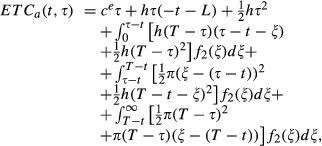
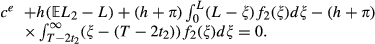
The calculation of the inventory holding cost and backorder cost depends on the completion time of the first stage, the arrival time of the expedited order, and the completion time of the second stage. We assume that T > 2L. There are a total of seven cases we need to consider.
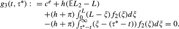
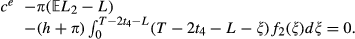
(a) t ≤ − ‰L: This is the case when the first stage completion time is well ahead of the demand season and the expedited units, if any, arrive before the demand interval starts. Denote ETC
a
(t, τ) as the expected total cost, if the first stage is finished at time t and the expediting quantity is τ, with the subscript “a” corresponding to case (a). Then,
The first‐order condition (FOC) of ETC
a
for an interior solution


It can be shown that the expected total cost ETC
b1 is linear in τ with a slope of k
1 given as follows:
The expected total cost ETC
b2 is convex in τ, and the first order condition can be characterized by (FOC1). ETC
b3 can also be shown to be convex in τ, and its first‐order condition is given as follows:
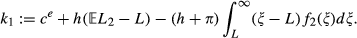
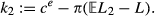
Similarly, we can calculate the expected total cost for other cases. We summarize the characterizing equations and slopes in Table 1. For understanding this table we need two other first order conditions (FOC3) and (FOC4), and a constant k
2 representing a slope, which are defined as follows:
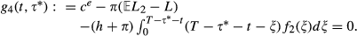
Details of the Seven Cases of ETC Calculations: First‐Order Conditions and Slopes
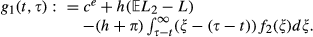
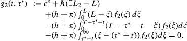
The following lemmas present the properties of g i (t, τ) (i = 1, 2, 3, and 4) and the expected total cost.
g
1(t, τ) is increasing in τ and decreasing in t.
g
2(t, τ) is increasing in τ.
g
3(t, τ) is increasing in τ and decreasing in t.
g
4(t, τ) is increasing in both τ and t.
The expected total cost is convex in τ for any given t.
Lemma 2 can be proved by evaluating the derivatives of the expected total cost function from the left and from the right at the adjoining points of every two adjacent regions. Since the expected total cost is piecewise convex in τ and the derivative is continuous, the expected total cost must be convex in τ in the whole domain [0, T].
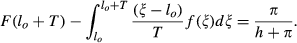
First, with a high expediting cost, the expediting option will not be used. The following proposition characterizes the threshold value of the expediting cost above which the expediting service is considered prohibitively expensive.
If


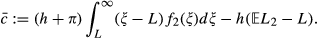
The proofs of all propositions are included in Appendix A. Note that 
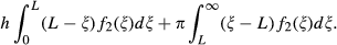
This is the standard expected loss function 


Next, we will derive the optimal expediting policy when the expediting cost c
e
is below a certain threshold. To proceed, we define 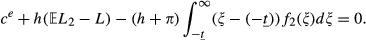
Through this section and the next, we assume that
Let 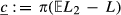


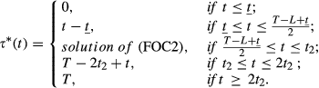
Figure 1a illustrates the form of the optimal expediting policy when the expediting cost c
e
is lower than 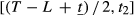
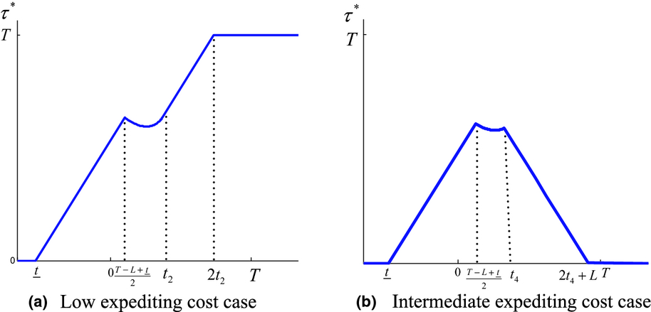
Illustration of Optimal Expediting Policy (L 1, L 2 ∼ exp(1), h = 1.5, π = 5, T = 3, L = 0.8, c e = 1 in (a) and c e = 1.2 in (b))
We now examine the nature of the optimal expediting policy within the so‐called “middle interval” 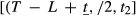

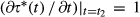


As shown in Figure 1a, within the middle interval, the principle of “longer delay leads to more expediting” (i.e., a later realization of the first stage completion leads to a larger portion being expedited) might break down.
Next, we will derive the optimal expediting policy when the expediting cost c
e
is between 
The following proposition characterizes the optimal expediting policy.
If 

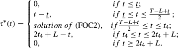
Figure 1b illustrates the form of the optimal expediting policy when 


First, we study how the cost and lead‐time of the expediting service affect the optimal expediting policy.
In the low expediting cost case (i.e.,
Both

With everything else remaining the same, a lower premium makes the expediting option more profitable and leads to its increased use. But for a small expediting lead‐time L, a further reduction might dampen the incentive to expedite. Speeding up the delivery of the expedited units elongates their time in inventory and increases the corresponding holding cost. Similarly for the intermediate expediting cost case, we have the following proposition.
In the intermediate expediting cost case (i.e.,

Note that although a shorter expediting lead‐time dampens the incentive to expedite early in the horizon as in Proposition 4, as L decreases, the threshold 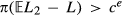
Next, we study how the inventory‐related costs affect the optimal expediting behavior.
In the low expediting cost case (i.e.,
Both Both 
We see that a higher backorder cost induces more expediting. However, the inventory holding cost has two effects: an increase in the unit holding cost will penalize whichever of the ordered units, through regular or expedited delivery, arrive first. When the expediting cost is low, the increase in the unit holding cost impacts the expedited units the most, thus arguing for higher unit holding cost dampening the incentive for expediting. This is because our optimal policy suggests rather “aggressive expediting” (i.e., expedite earlier and have a higher likelihood to expedite the whole order). As shown in the next result, in the case when 
In the intermediate expediting cost case (i.e., 
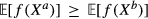
It is also interesting to study the effect of the regular lead‐time variability on the expediting policy. To do so, we introduce the notion of increasing‐convex ordering (see Ross 1983): Let X
a
and X
b
be two non‐negative random variables such that 
Let L
2
a
and L
2
b
be two random variables for the second stage lead‐time such that 


The above result implies that a more variable lead‐time expands the expediting region when 

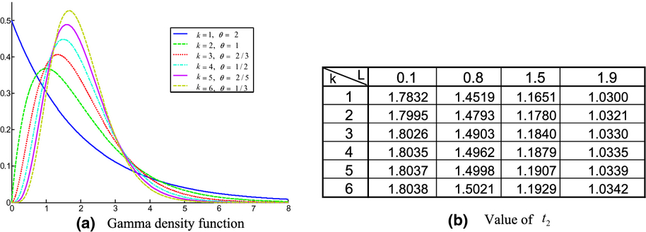
Impact of Variability of L 2 on t 2 for Gamma Distributions (h = 1.5, π = 5, T = 4, L = 0.8, kθ = 2)
From Proposition 2 and 3, we see that within the middle interval, finding the optimal expediting quantity involves solving an integral equation which makes the optimal policy difficult to calculate. One reasonable heuristic that approximates the optimal expediting policy is to ignore the middle interval. In the low expediting cost case (
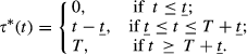
Figure 3a illustrates the form of the heuristic policy and Figure 3b illustrates its performance. The solid line represents the optimal expediting policy and the corresponding expected total cost. The dashed line shows the heuristic policy and the corresponding expected total cost. The dotted line on Figure 3b shows the expected cost if the expediting option is not available. Here, we assume that, under both the optimal and heuristic policy, the regular replenishment order is placed at time −l, where l is the optimal safety lead‐time without the expediting opportunity (optimally choosing a safety lead‐time will be discussed in section 4). As shown, the heuristic policy can achieve 92–94% of the overall cost savings brought by the optimal policy. The proofs of Proposition 4 and 6 imply that the heuristic works the best when c e and h are big or when L and π are small (since the length of the middle interval will be small). This is what we observe in Figure 3b: the gap between the heuristic policy and the optimal policy is smaller the higher c e is.
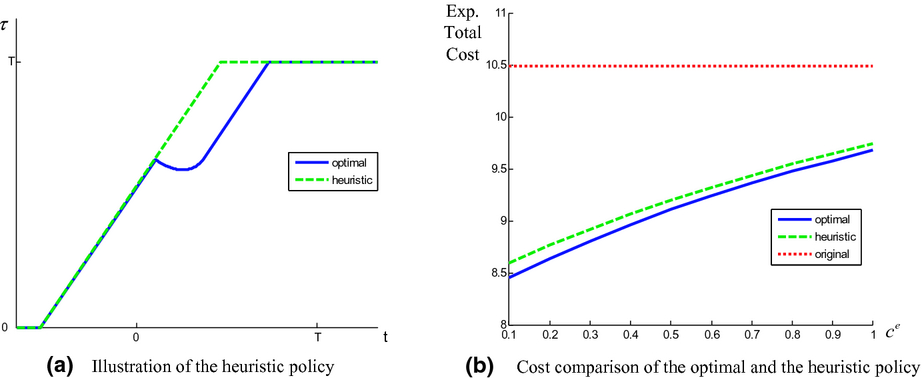
Illustration of the Heuristic Policy for Low Expediting Cost Case (L 1, L 2 ∼ exp(1), h = 1.5, π = 5, T = 3, L = 0.8)
Similarly, a simple heuristic policy for the intermediate expediting cost case (
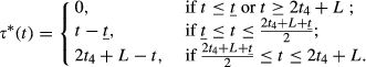
The form of the heuristic policy is shown in Figure 4a. The solid line represents the optimal expediting policy and the dashed line the heuristic policy. Since the middle interval is narrower in the intermediate expediting cost case, the heuristic policy behaves even better than its counterpart in the low expediting cost case. It can achieve 95–98% of the overall cost savings. The proofs of Propositions 5 and 7 imply that the heuristic performs the best when c e is big, or h and π are small, since the length of the middle interval decreases in c e and increases in h and π.
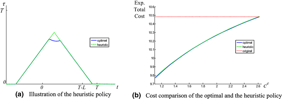
Illustration of the Heuristic Policy for Intermediate Expediting Cost Case (L 1, L 2 ∼ exp(1), h = 1.5, π = 5, T = 3, L = 0.8)
In the above analysis, we assumed that the deterministic expediting lead‐time is shorter than the regular lead‐time L 2 on average. This implies that the expediting service may take longer than the regular lead‐time. Now, we consider the case that the expediting service guarantees a shorter lead‐time.
Let L
2 = L + ε, where ε is a non‐negative random variable with pdf g
2(·) and cdf G
2(·). Define 
Then the optimal expediting policy can be characterized as follows.
If L
2 = L + ε, where ε is a non‐negative random variable, then the optimal expediting policy can be given as follows:
If If


Note that the optimal policy (11) is equivalent to the heuristic policy (9) and is illustrated in Figure 3a. The fact that the expediting service guarantees a shorter lead‐time changes the optimal expediting policy in two ways. First, the “conservatively expedite” region disappears. We have seen in Proposition 1 that, when the expediting cost c
e
is higher than the expected loss of not expediting, the expediting service will not be used at all. Here, since the expediting service guarantees a shorter lead‐time, the expected loss of not expediting only includes the expected backorder cost 

Effect of Expediting on the Safety Lead‐Time
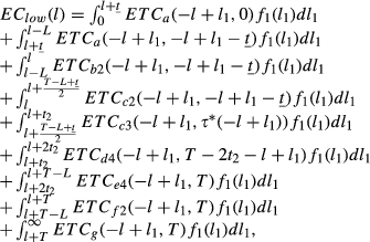
Without the presence of the expediting service, in choosing the safety lead‐time, the retailer minimizes the expected total cost: 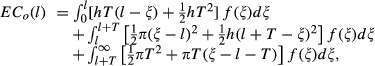
In the presence of the expediting service, if the retailer uses the service according to the optimal policy derived in section 3, then the expected total cost viewed at the time when the replenishment order is placed, that is, at time −l, can be calculated as follows: If the expediting cost is too high, that is, 


The following parameters are used in Figure 5. The expediting lead‐time is fixed at L = 2; the first lead‐time component has a Gamma distribution with shape parameter k
1 = 4 and scale parameter θ
1 = 1, and the second lead‐time component has a Gamma distribution with shape parameter k
2 = 2.5 and scale parameter θ
2 = 1; the order size is T = 6; and the inventory‐related costs are h = 1.5, π = 5. The two threshold values 

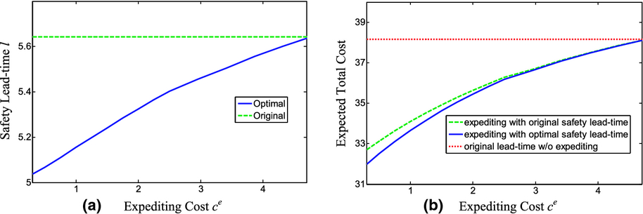
Effect of Expediting on Safety Lead‐Time and Expected Cost (h = 1.5, π = 5, L 1 ∼ Gamma(4, 1), L 2 ∼ Gamma(2.5, 1), T = 6, L = 2)
Figure 5b compares the expected total cost. As a benchmark, the expected total cost without expediting and with the original safety lead‐time determined by Equation (13) is shown by the dotted horizontal line. The solid line is the expected total cost with expediting and the optimal safety lead‐time obtained in Figure 5a. The gap between these two curves indicates the value of expediting. Though choosing the optimal safety lead‐time results in the least expected total cost, it requires higher computational effort. Figure 5b also shows the comparison of the expected total cost under the optimal safety lead‐time l * (the solid line) and under the original safety lead‐time l o (the dashed line). As we can see most of the cost savings result from using the expediting option in an optimal way. The additional benefit from optimizing the safety lead‐time is significantly smaller, in most cases < 10%, as in our example.
In our discussion so far, the order size T was exogenously given. When there are economies of scale in ordering (e.g., a fixed ordering cost), choosing the right order size becomes important. Denote the fixed ordering cost to be K and the variable cost v. Then the expected average cost per period is: 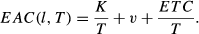
Figure 6 shows the per period expected cost when expediting is used and the safety lead‐time is chosen optimally for different values of T in the following setting: L 1 ∼ Gamma(4, 1) and L 2 ∼ Gamma(2.5, 1), expediting lead‐time L = 2, expediting cost c e = 3, inventory‐related cost h = 1.5, π = 5, fixed ordering cost K = 10, and variable ordering cost v = 1.5. We observe that the expected average cost preserves the robustness property of the traditional EOQ model. That is, a small deviation from the optimal size will not increase the expected cost by much. Hence some simple near‐optimal heuristic may perform well. One candidate is the EOQ quantity. In our numerical example, the EOQ quantity is T EOQ = 7.6012, which is 25% higher than the optimal order size T * = 6.0941. But the expected cost under T EOQ is only 1.3% higher than the minimum expected cost per period.
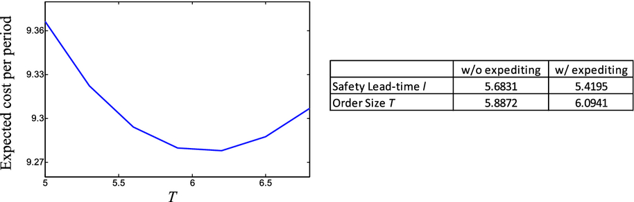
Expected per Period Cost for Different Order Size T and Comparison of Optimal and Original Safety Lead‐Time and Order Size (h = 1.5, π = 5, K = 10, ν = 1.5, L 1 ∼ Gamma(4, 1), L 2 ∼ Gamma(2.5, 1), L = 2, c e = 3)
The small table next to Figure 6 reports the optimal safety lead‐time and order size with and without expediting. We observe that the presence of the expediting service leads to an increase in the order size and at the same time a decrease in the safety lead‐time. In other words, the optimal use of expediting service will support the placement of larger replenishment orders, thus taking increased advantage of economies of scales and using smaller safety lead‐times, which adds to the system responsiveness.
In section 3, we analyzed the model in which the two lead‐time random variables L 1 and L 2 are independently distributed. This is reasonable when the two lead‐time stages have very different nature and the corresponding processes are managed by different parties. For example, the first stage represents production and the second stage represents transportation part of the lead‐time. However, when the majority of the lead‐time consists of transportation time and L 1 and L 2 correspond to two phases of the transportation activity, these two lead‐time stages are usually correlated. They may be negatively correlated, for instance when the logistics manager sees a delay in the first phase, he may assign the best resource to handle the second phase so that the realization of L 2 is likely to be small. In other cases, L 1 and L 2 may be positively correlated, when the uncertainties in the two lead‐time stages are due to the same or a similar factor (e.g., union strike, weather condition, safety inspection, etc).
To analyze the effect of correlated lead‐times, we adopt the simple discrete joint distribution framework considered in Babich et al. (2007) in modeling supply risk. We assume that L
1 can take one of two values l
1L
and l
1S
, where l
1L
> l
1S
and the subscript L and S represent long and short, respectively. For simplicity, we use the same assumption as section 3.5 for L
2. That is, L
2 = L + ε, where L is the deterministic expediting lead‐time and ε is a positive random variable. Similar to L
1, we assume that ε can take one of two values e
L
and e
S
, where e
L
> e
S
. Use p
ij
, (i, j = 0, 1) to represent the joint probability of (L
1, ε). If the lead‐time takes the longer time, the corresponding value of i or j equals 1. For example, p
01 denotes the joint probability of L
1 = l
1S
and ε = e
L
. This joint distribution is completely characterized by the two marginal probabilities ϕ
1 = p
10 + p
11, ϕ
2 = p
01 + p
11, and the joint probability p
11. By setting 

In Proposition 9, we see that the expediting decision depends on the realized value of L
1, or equivalently t (t = −l + L
1). So let us first assume that the first lead‐time stage takes the longer time, that is, L
1 = l
1L
. Given this, the conditional probability for L
2 can be expressed as: 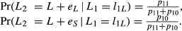
By Proposition 9, the optimal expediting quantity also depends on the threshold value 
It can be easily seen that 

Similarly, if L
1 = l
1S
, the conditional probability for L
2 can be expressed as 


Since 
Three Lead‐Time Stages
Finally, we extend our basic model to include more than two lead‐time stages reflecting the case where the regular shipment stops more than once during the supply process. The question we address is: If there is a one‐time opportunity to expedite part or all of the shipment, should it be used earlier or later? Due to computational complexity, we restrict ourselves to the case where the expediting service guarantees a shorter lead‐time. Particularly, let L i = m i + ε i be the ith stage of the lead‐time (i = 1, 2, 3), where m i is a constant and ε i is a non‐negative random variable. If one decides to expedite at the first breakpoint when L 1 is realized, then the expediting lead‐time is assumed to be m 2 + m 3. If one waits until the shipment goes through the second breakpoint and makes the expediting decision at that time, then the expediting lead‐time is denoted by m 3.
In our numerical examples below, the following parameters are used: ε i is normally distributed with mean m i and standard deviation m i /3 (so the probability of ε i < 0 is small). The cost parameters are: c e = 4, h = 4, π = 3, T = 10, and l = 12. To study the timing issue of expediting, we first fix the location of the first breakpoint and show the optimal expediting decision for different locations of the second breakpoint. For that we fix m 1 = 2 and consider the following three scenarios: case (1) m 2 = 1, m 3 = 5; case (2) m 2 = 3, m 3 = 3; and case (3) m 2 = 5, m 3 = 1, corresponding to the second breakpoint closer and closer to the destination. Figure 7a compares the optimal expediting decisions for the three scenarios, where “0” denotes “shipment has no delay so no need for expediting,” “1” denotes “expedite right now,” and “2” denotes “shipment has delay but it is more profitable to wait until the next stop and make a decision then.” We observe that if the shipment has only a small delay when it goes through the first breakpoint, it is worthwhile to hold the expediting opportunity until more information about the lead‐time is revealed at the second stop. However, the wait option becomes less and less attractive when the second breakpoint is located closer and closer to the destination. The information simply becomes less valuable as the shipment gets close to the destination. Any expediting may not help much.
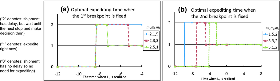
Optimal Expediting Decision when there Are Three Lead‐Time Stages
We also perform the same analysis when the location of the second breakpoint is fixed while the location of the first breakpoint varies. For that we fix m
3 = 2 and consider the following three scenarios: case (1) m
1 = 1, m
2 = 5; case (2) m
1 = 3, m
2 = 3; and case (3) m
1 = 5, m
2 = 1, corresponding to the first breakpoint further and further away from the origin. Figure 7b shows the optimal expediting decisions for the three scenarios. For each scenario, the graph shows the period when 
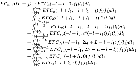
In contemporary global supply chains of “functional goods,” low‐cost‐driven outsourcing from far away suppliers results in challenges to managing long and highly variable lead‐times. In our research we studied the use of order expediting in response to partially resolved lead‐time information in a situation where the lead‐time of a retailer's replenishment orders to meet his constant demand rate consists of two stages. Each stage has a random duration. At the completion time of the first supply stage, the retailer can expedite at a cost premium a portion of his earlier placed order, with the expedited portion arriving in a deterministic lead‐time that is shorter than the average duration of the second stage. To facilitate our study, we assumed that the retailer assigns an interval of demand to each order and thus we focused our study only in a demand interval that is planned to be satisfied from an order placed earlier before the demand starts.
For the situation considered, we formulated the expected total cost of meeting demand for a given safety lead‐time, whose calculation depends on the completion time of the first stage, viewed at the time of the expediting decision. We showed that the expected total cost is convex in the expediting order quantity and that the optimal expediting policy can be characterized explicitly. Two thresholds on the unit expediting cost define three regions of the expediting policy. When expediting is too expensive, it will never be used. When expediting is very cheap, it is optimal to fully exploit the expediting opportunity and use it aggressively (expediting the whole order for extremely long delays). When the expediting cost is in between, it is optimal to adopt the expediting service but only leverage it in a limited way (beyond a certain delay level, decreasing the expedited portion as delay increases). It was observed that the optimal expediting policy does not necessarily have simple monotonicity in the first stage completion time, particularly when the completion of the first stage falls in the so‐called “middle‐interval.” Heuristic policies were presented to simplify the calculation of the expediting policy and numerical examples suggested that the performance of the heuristic policies is satisfactory. It was noted that if the expediting option guarantees a shorter lead‐time than the second stage, then the intuition of “longer delay leads to more expediting” restores.
The impact of some basic model parameters on the optimal expediting policy was studied. In particular, a lower cost of the expediting service, a higher backorder cost, or a more variable supply lead‐time leads to a higher propensity to use the expediting service (i.e., expedite earlier and higher portions). The impact of unit holding cost on the optimal expediting policy depends on the cost of the expediting service. For a low expediting cost, an increase in inventory holding cost reduces the use of expediting (i.e., expedite later and smaller portions). In the intermediate cost case, the opposite occurs with expediting becoming more of an attractive option. Another seemingly counter‐intuitive result is that a decreasing expediting lead‐time might reduce the incentive to expedite and lead to delayed expediting and lower likelihood to expedite the whole order, especially so for small delays in the first supply stage.
We also formulated the expected cost of meeting demand for a given safety lead‐time viewed at the time of placing the order. Numerical examples showed that with the expediting option, the optimal safety lead‐time is smaller than that without the expediting option, and the difference between the two safety lead‐times could be significant. Our study also suggested that the presence of the expediting option supports the placement of larger replenishment orders. However, the marginal benefit of simultaneous optimization of the safety lead‐time and order size is insignificant. So from a planning perspective, the timing and quantity decision for the regular replenishment order can be made without taking into account the expediting option. The focus should be on the careful exercise of the expediting option, as outlined in the optimal expediting policy (or the heuristic policy for practical purposes). We extend our basic model to consider correlated lead‐time stages and in a simple discrete joint distribution model, we see that for positively (negatively) correlated lead‐times, one would count more (less) on the expediting service when there is a delay. Finally, we show that when the replenishment lead‐time consists of more than two stages, the one‐time expediting option should be exercised to respond to shipment delays when enough information is revealed and when it is not too late.
Our research prescribes for logistics managers the optimal way of utilizing an expediting service and offers important insights on factors that may affect their expediting decisions. More importantly, our work provides a useful model to help quantify the value of detailed supply information, hence can be used to evaluate whether and where to install some advanced information technology equipment, such as RFID, in an effort to obtain such real‐time supply information. Further research should try to better understand how differently an expediting service should be used to manage “innovative” products (Fisher 1997) rather than “functional” products studied in this research. Innovative products are characterized by less predictable demand, hence it is necessary to factor demand uncertainty in the analysis. Also, Wang et al. (2010) suggests that demand and lead‐time may be correlated. This may also affect the use of expediting service. Finally, we assume that the expediting service has a deterministic lead‐time. It could be interesting to see how to make use of a service with random expediting lead‐time.
Footnotes
Proofs
Expressions for Expected Total Costs
Acknowledgments
We are grateful to the anonymous reviewers, the Senior Editor, and Departmental Editor J. George Shanthikumar for their valuable comments. We also would like to thank Jian Li for his help in improving the paper, and the support from the Boeing Center for Technology, Information and Manufacturing (BCTIM).
1
It can be shown that (T ‐ L ‐ṯ) / 2 < T, since ṯ < ‐ (T ‐ L) by assumption. Also, in the proof for Proposition 3, it is shown that t4 < (T ‐ L)/2. So (t4 +L) (T + L)/2 < T, where the last inequality follows from the model assumption T < 2L.