
Abstract
We develop, in this article, a sales model for movie and game products at Blockbuster. The model assumes that there are three sales components: the first is from consumers who have already committed to purchasing (or renting) a product (e.g., based on promotion of, or exposure to, the product prior to its launch); the second comes from consumers who are potential buyers of the product; and the third comes from either a networking effect on closely tied (as in a social group) potential buyers from previous buyers (in the case of movie rental and all retail products) or re‐rents (in the case of game rental). In addition, we explicitly formulate into our model dynamic interactions between these sales components, both within and across sales periods. This important feature is motivated by realism, and it significantly contributes to the accuracy of our model. The model is thoroughly tested against sales data for rental and retail products from Blockbuster. Our empirical results show that the model offers excellent fit to actual sales activity. We also demonstrate that the model is capable of delivering reasonable sales forecasts based solely on environmental data (e.g., theatrical sales, studio, genre, MPAA ratings, etc.) and actual first‐period sales. Accurate sales forecasts can lead to significant cost savings. In particular, it can improve the retail operations at Blockbuster by determining appropriate order quantities of products, which is critical in effective inventory management (i.e., it can reduce the extent of over‐stocking and under‐stocking). While our model is developed specifically for product sales at Blockbuster, we believe that with context‐dependent modifications, our modeling approach could also provide a reasonable basis for the study of sales for other short‐Life‐Cycle products.
Keywords
Introduction
Forecasting sales is an important task for most firms. This task can in fact be critical for the survival of companies that deal with innovative, very‐short‐life‐cycle products. Blockbuster is one such company in the rentable‐DVD and game‐media industry. With over 6500 stores in 18 countries (4018 in the United States including franchisees), its annual revenue for fiscal year 2009 is over $4.06 billion, of which more than 60% is attributed to DVD rentals (Blockbuster Incorporated 2009). Industry wide, DVD movie rental and retail (i.e., outright product purchases) activity generated over $24.1 billion in sales in 2006, and rental and retail sales for game software exceeded $6.5 billion annually (Blockbuster Incorporated 2006). Our objective in this article was to develop an effective sales forecast model for short‐life‐cycle products, such as those found at Blockbuster.
The primary sales characteristic of products in the DVD and electronic game industry is that they have highly compressed life cycles. The short active life span is inherent in any entertainment media product. It is customary for products in this industry to realize the majority of sales in the first few weeks they are offered. This high initial sales volume is typically followed by quickly declining sales in subsequent weeks. However, it is also not uncommon to find products that have sales trajectories which exhibit either a classical diffusion pattern (Bass 1969, Mahajan et al. 2000, Niu 2002, Rogers 2003), manifested as a later period increase in sales, or some other characteristics that are altogether different, such as post first period sales spikes. Thus, the DVD and electronic game industry can be viewed as one with highly compressed product life cycles that have little correlation to traditional product seasons. Furthermore, as each product is unique and original, no reliable benchmarks can be used to predict sales of specific products. As a result of these difficulties, the industry has developed an innate, deep‐rooted skepticism regarding the use of decision support systems. This backdrop provides a strong motivation for the development of reliable forecasting approaches.
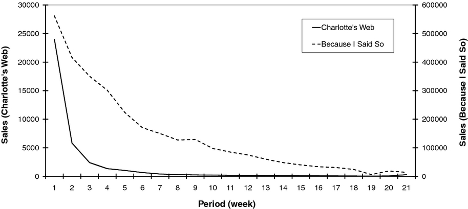
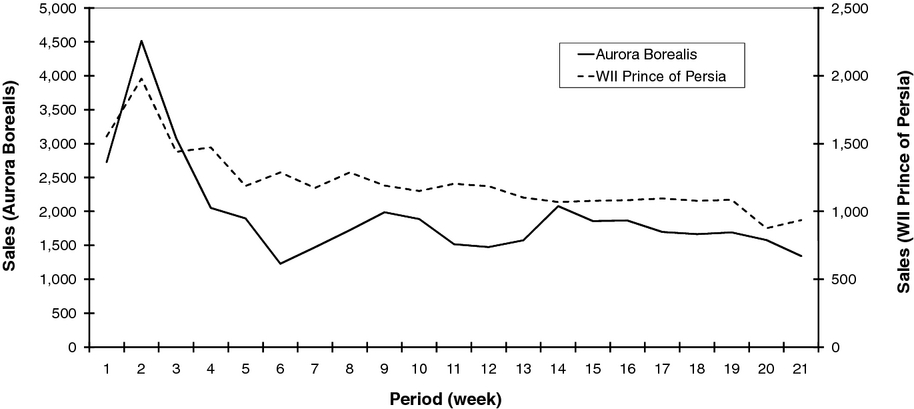
The challenge in forecasting sales in this industry can be illustrated by several generic product examples. For newly released DVD and game products (retail or rental), weekly sales for many titles follow what appears to be a pure exponential‐decay pattern. In Figure 1, the titles “Charlotte's Web” and “Because I Said So” both exhibit steadily declining sales. Notice, however, that there is a subtle difference between the two, in that the latter has a heavier tail for an extended duration, suggesting that some “hidden” sales components may be at play. With somewhat less frequency, there also exist sales patterns that are much different from exponential. In Figure 2, sales for the titles “Aurora Borealis” and “WII Prince of Persia” are interesting examples where the second‐period sales are significantly higher than those of the first. Moreover, while there exist signs of an exponential decay after the second‐period spike, sales in later periods appear to be primarily driven by some “non‐apparent” forces. These disparate sales patterns clearly demonstrate that accurate sales forecasting is difficult.
Exponential Sales Pattern
A further challenge in this environment is that it is important to get the forecast right in the first several periods of product sale. If the company under‐forecasts in the early periods, it would experience lost sales that, due to the competitive nature of the industry, could not be recouped in subsequent periods. In other words, any instance of under‐forecasting in the first few periods would have a negative impact on the profitability of a product. Conversely, any over‐forecasting would result in poor product utilization and hence unnecessary stocking and holding costs. As there are roughly 55 new releases at Blockbuster every week, accurate and timely sales forecasts can significantly reduce operating costs.
Non‐Exponential Sales Pattern
In this article, we will first formulate a sales model for movie and game products at Blockbuster and then, after validation, use the model to develop sales forecasts.
Our model formulation is based on a decomposition of the total sales into three components. The first component is due to consumers who are strongly committed to purchasing the product. The second is due to consumers who are potential buyers (whose purchase decisions could be influenced by previous buyers). The third is due to either a networking effect from previous buyers on their closely tied social groups or re‐rents. This decomposition is motivated by and helps explain the observed diverse sales patterns at Blockbuster. Another important feature of our model is that we allow dynamic interactions between these sales components within each sales period as well as period‐by‐period updates of model parameters.
The sales model is tested against extensive sales data from Blockbuster. It fits actual sales extremely well. With the model validated, we also demonstrate that when used in conjunction with publicly available environmental data, such as theatrical sales, studio, genre, MPAA ratings, etc., it is capable of delivering reasonable sales forecasts. We further develop a method that can be used to adjust and improve the initial forecasts based on actual first‐period sales, which can help Blockbuster to respond to any discrepancies in the initial order. As noted previously, excessive initial over‐ or under‐stocking of products has negative cost consequences. Therefore, our forecasting method has the potential to enhance revenue and reduce cost for Blockbuster.
Our work provides several useful contributions to the extant literature (see section 2). The explicit formulations of three sales components, the interaction between these components, and the dynamic parameter updates, are novel. When coupled with good quality input data, our model can be used to conduct sales forecasts, which could lead to better purchasing and inventory decisions for Blockbuster's retail operations (see section 4.4). Finally, the sales decomposition is quite generic, and therefore, can be used in the modeling of sales for short‐life‐cycle products in other scenarios.
The remainder of this article is organized as follows. In section 2, we review some of the available literature. Sections 3 and 4 are devoted, respectively, to model development and to an empirical study on the performance of our model, using actual sales data from Blockbuster. Section 5 contains concluding remarks.
Numerous approaches for forecasting sales have been studied in the literature. Most of the methods are developed for settings that are not specific to short‐life‐cycle products, and a significant number of them are based on the Bass Model (BM; Bass 1969). We will therefore begin with a brief review of the BM, focusing on its main idea and some related variants. This is followed by a summary of other methods. We then conclude this section with a discussion of what we consider as important modeling features for short‐life‐cycle products.
Bass originally envisioned a single large potential‐adopter population. In his model, it is assumed that each potential adopter in this population has an instantaneous adoption (i.e., purchasing) rate that depends on two forces. The first force is due to an intrinsic interest in the given product, independent of the number of previous adopters, and the second is due to a positive influence from previous adopters. This leads to a differential equation (involving two parameters denoted by p and q that correspond to these two forces) for the fraction of potential adopters who would have adopted by time t, for t ≥ 0 (Bass 1969, p. 217, or Niu 2006, p. 679). For a given “large” population size, the solution of this differential equation then yields an S‐shaped cumulative‐sales curve. As this solution is deterministic, a sequence of independent and identically distributed (i.i.d.) error terms is finally added to this model to yield successive sales over given time periods (of same duration).
Bass interprets these aforementioned forces as originating from the distinction between “innovators” (or early adopters) and “imitators” (or late adopters). Interestingly, an earlier 1962 edition of Rogers's text actually provided the motivation behind his formulation (see Bass 1969, p. 215). This primitive notion of innovators vs. imitators can be formalized in a number of different ways. Some examples of these can be found in a review by Hardie et al. (1998), and in related work by Mahajan et al. (1990), Niu (2002, 2006), Rogers (2003), Schmidt and Druehl (2005), Tanny and Derzko (1988), and Van den Bulte and Joshi (2007). As will be seen in section 3 below, the formulation of our model, which extends Niu (2006), is also related to this notion (see the committed‐ and potential‐buyer populations in section 3).
In their review of the general literature, Hardie et al. (1998) surveys eight forecasting methods. They test all eight methods against 19 data sets from a variety of products to determine which methods work better, and under what settings. The products in their data sets are items such as shelf‐stable juices, cookies, salty snacks, and salad dressings. Their results show that the BM performs well compared with other forecasting methods.
Rogers (2003) and Mahajan et al. (1990) present distinctly different approaches on how to treat different populations. Bass conceptualized the innovator and imitator populations as purchasing concurrently throughout the life cycle. In contrast, Rogers (2003) conceptualized these populations as being time sequential, meaning that early purchases were due to one population and later purchases were due to the other. In other words, the two populations do not have concurrent purchase activity. Similar to Rogers (2003), Mahajan et al. (, p. 1990 describe how the innovator and imitator populations coalesce into time sequential purchasing populations. A related comparison of these formulations can also be found in Mahajan et al. (2000), where the authors further discuss the innovators‐vs.‐imitators concept.
Another interesting fact regarding the Bass formulation is that it does not segregate the innovator and imitator populations. In an attempt to better understand the effect of having an explicit segregation of these two populations, Tanny and Derzko (1988) propose and test a “two‐compartment” model. They conclude that their model does not lead to superior empirical performance over the BM.
Continuing the spirit of Tanny and Derzko (1988) and other related work (e.g., Steffens and Murthy 1992), Van den Bulte and Joshi (2007) studied a model that has two distinct market segments, namely influencers and imitators (analogous to innovators and imitators). They assume that these populations make purchases concurrently and that there is an asymmetric influencing effect from the influencers onto the imitators. Both these features (i.e., having two concurrent populations and allowing interactions between the populations) are desirable improvements over previous work.
We now provide a summary of a number of other forecasting models. Several of them are developed for music titles and theatrical movie releases, which are in some regards similar to Blockbuster's products. In particular, they also have short life cycles.
Garber et al. (2004) present a model for the rate of product sales based on the notion of a “localized sales density.” The authors posit that if the density of product purchasers within a geographical area is high enough, then a word‐of‐mouth effect will become very strong, resulting in what they refer to as a “contagion process.” Conversely, if the density of purchasers within a geographical area is low, then momentum behind product sales diminishes rapidly.
Jedidi et al. (1998) analyzed box office releases using an exponential‐decay model. They developed a technique that categorized a new movie as a member of one of four mutually exclusive movie clusters, where the clusters differ in opening strength and decay rates.
Moe and Fader (2001) studied weekly music sales, also using an exponential‐decay model. Similar to Jedidi et al. (1998), they associated each product with a “cluster,” but they developed a more rigorous approach. In Moe and Fader's model, each cluster had two parameters, namely a constant rate of purchase and a market‐penetration level. These parameters were estimated from past performance of products in that cluster. Sales forecasting then involves the classification of to which cluster a new product belongs, and applying the parameters from that cluster.
Sawhney and Eliashberg (1996) modeled an individual's time to see a movie as the sum of two random variables, namely the time to decide to see the movie and the time to act on the decision. The authors also assumed that these time intervals are independent, meaning that the time it takes to decide does not influence how fast an individual will act and vice versa. From their empirical analysis, the authors observed that it was reasonable to assume that the distributions of these time intervals are exponential, Erlang, or gamma. Indeed, the authors had good success at forecasting sales given only two or three actual sales data points.
Eliashberg et al. (2000) developed a model called MOVIEMOD to forecast box office movie performance. In this model, it is assumed that, prior to the release of a movie, individuals (potential consumers) can be in one of six possible “behavioral” states, namely undecided, considerer, rejecter, positive spreader, negative spreader, and inactive (Mahajan et al. 1984). All consumers begin in the undecided state and may evolve over time to other states according to an “interactive” Markov chain (Conlisk 1976). The formulation by Eliashberg et al. (2000) reflected the impact of word‐of‐mouth interactions between individuals, marketing activities, and movie experience. Their model was calibrated using consumer clinic experiments, and the resulting forecasts worked quite well.
Lee et al. (2003) and Ainslie et al. (2005) both utilized a hierarchical Bayesian framework for forecasting sales. In Lee et al. (2003), a model was developed to forecast music album sales prior to an album's release; and in Ainslie et al. (2005), a model was developed to forecast movie theatrical performance when consumers have the ability to choose from one of multiple movies. Both papers allowed for dynamic population sizes and sales updates between periods as actual data becomes available, and this was made possible by the Bayesian framework.
Lastly, in Lilien et al. (1981), Hahn et al. (1994), and Fader et al. (2004), a variety of forecasting techniques for consumable products (for example, peanut butter) were considered. For such products, there existed a significant amount of repeat purchases. Clearly, demands for consumables were quite different from that of innovative, short‐life‐cycle products, such as DVD or game products.
The prior work cited above is clearly valuable in furthering research in sales forecast models. However, our primary focus in this article was on movie and game products, which have short life cycles. For such products, we believe that it is important for the model to capture three main features: (i) formulation of multiple consumer sub‐populations, (ii) allowing interactions between consumer sub‐populations, and (iii) having dynamic parameter updates over time, both within each sub‐population and across different sub‐populations. Feature (i) is similar in spirit to Tanny and Derzko (1988); in our setting, the primary rationale is that some consumers may have already been exposed to the product (or product information) and therefore have formed an opinion that is strong enough to alter their purchase behavior. Both (ii) and (iii) are, similar to the BM, motivated by the fact that existing buyers of a product have a dynamic influence over the entire residual population; moreover, these two features are of particular importance for short‐life‐cycle products because such products typically have rapidly changing sales trajectories. To the best of our knowledge, a sales forecast model that satisfactorily addresses these features does not appear to be available in the literature. This perhaps is due in part to the difficulty in the formulation of features (ii) and (iii).
In this article, we will develop a sales model that incorporates all three features above. The construction of our model relies closely on recent stochastic extensions of the BM by Niu (2002, 2006). The model is presented in the next section.
The Model
To facilitate understanding, we begin with some informal motivation. Our basic proposition is that DVD and game sales for both rental and retail products can be effectively modeled by considering three sales components that are derived from two distinct consumer populations.
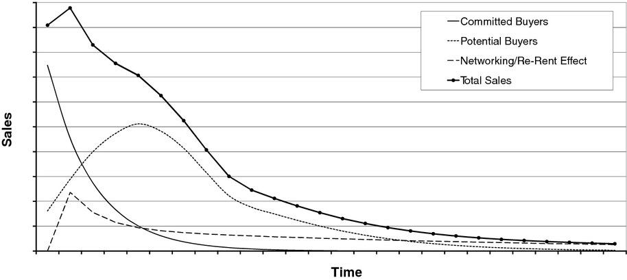
First, we assume that there is a sales component due to a segment of consumers who have already decided to purchase (or rent) a product after its release (possibly due to prior exposures to the product, e.g., the theatrical release of a movie or prelaunch advertising). We refer to this segment as committed buyers. As committed buyers have already made their decisions a priori, we will further assume that the timing of their purchases is independent of the rest of the population. More specifically, we define each period as a week, and postulate that the trajectory of weekly sales from this segment of consumers decays exponentially over time according to an intrinsic purchase rate. This is illustrated in Figure 3 as the committed‐buyers curve.
Decomposition of Total Sales
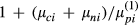
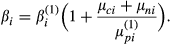
Second, we assume that there is a sales component due to a segment of consumers whose purchase timing follows a bell‐shaped diffusion curve. We will refer to this segment of consumers as potential buyers. In contrast to the committed buyers, we assume that successive weekly sales from this segment of consumers depend on a pair of recursively updated purchase rates, both of which are tied to the extents of the intrinsic interest in the product and of the force of the unidirectional influencing effect from an existing buyer. A typical sales trajectory of this segment of consumers is illustrated by the potential‐buyers curve in Figure 3.
Lastly, we assume that there is a tertiary sales component due either to the effect of networking within a closely tied group of consumers in the case of DVD rentals and all retail products, or to re‐rents in the case of game rentals. This gives rise to two model variants, which we will refer to as the Networking Model and the Re‐Rent Model.
In the Networking Model, we assume that there is a networking effect, which explicitly takes into account the fact that current‐period sales may have a stronger impact in the subsequent period on the purchase activity of other potential buyers within their respective social groups. This is reasonable for retail and DVD rental products. The trajectory of this third sales component is shown as the networking/re‐rent effect curve in Figure 3. This curve exhibits no first period sales, a second period sales spike (which is due to the networking effect from those who bought in the first period), and finally an exponential‐looking decay. Note that the final decay is an aggregation of the impacts of the current sales from both the committed buyers and the potential buyers, and the precise trajectory of this decay is dependent on the relative sales strengths of these two populations.
In the Re‐Rent Model, which is for game rentals, we replace the networking effect by a re‐rent effect. Specifically, we postulate that a fraction of a given period's new renters will re‐rent in the subsequent period, and that the impact of re‐rents significantly dominates that of the networking effect, so that the latter could be ignored. These assumptions are reasonable because the intensity or difficulty of a game may entice a substantial number of new renters to rent again. The sales trajectory from this re‐rent effect is analogous to that from the networking effect, and therefore is also displayed as the networking/re‐rent effect curve in Figure 3.
When combined, these three sales components yield the total‐sales curve, which is also shown in Figure 3. In general, the resulting composite sales curve could exhibit some combination of (i) an initial peak (due to a high volume of sales to the committed buyers), (ii) a second period spike (due to the networking or re‐rent effect from the first period), and (iii) a late‐period uptick (due to the sales peak of the potential buyers).
We will present the detailed formulations of the Networking and the Re‐Rent Models in sections 3.1 and 3.2, respectively.
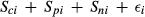
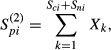
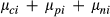
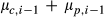
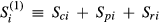
The Networking Model formulated here is for DVD and game retail, and for DVD rental products. We will assume that, for each of the periods i = 1,…,N, where N is a fixed horizon, there are three sales components,


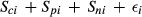
The total sales for period i,


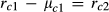
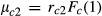
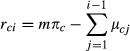
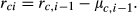
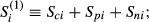
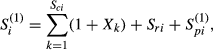
Now, define


The complete specification of (1) requires that we provide a full set of values for the


Formulation of the Means
We will start with the


Game Platform Sizes
Game Platform Sizes

To evaluate 


Beyond period 1, we shall find it convenient to define 


As a generic example, let us consider period 2. Observe that, at the start of period 2, the mean size of residual committed buyers 


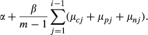
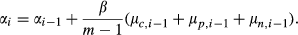
Repeating this argument then yields that for 1 ≤ i ≤ N, 

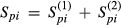
We now consider (2) as given and turn to the formulation of the 


Paralleling the committed‐buyer population, we will assume that the fraction of the market ceiling m that is considered to be potential buyers is 

For 1 ≤ i ≤ N, let 

We begin with period 1. We will first set 


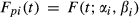
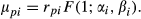
Consider a product that has a potential‐adopter population of size n (the term “adopter” is used here to avoid confusion with the terms “committed buyers” and “potential buyers” in our model). The SBM assumes that each potential adopter will purchase exactly one unit of the product, and that the cumulative number of adopters of the product evolves according to a pure birth process with state‐dependent birth rates. For any given n, the birth rates depend on two parameters, which are denoted by α and β. Specifically, it is assumed that if the current state (i.e., the total number of existing adopters) is j, where 0 ≤ j ≤ n, then the birth rate (i.e., the rate of time to next purchase) of the process is 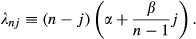
In (5), the first term n − j is the size of the residual potential‐adopter population. The second term is the rate for any of the residual potential adopters to make a purchase. The parameter α is an intrinsic purchase rate, independent of the existing adopters, for any of the potential adopters to make the purchase, given that the purchase has not yet been made; and its magnitude reflects the strength of the primitive appeal of the product. The parameter β is called the induction rate, and it reflects the strength of the total force of influence an existing adopter of the product has on the entire population. An important concept behind (5) is that the total induction force β from every existing adopter is apportioned uniformly to all other members of the entire population, so that each of the other members receives a share of magnitude β/(n − 1) (if a potential adopter has already made the purchase, the exerted influence is ignored). This apportionment is what explains why the existing adoption count j is multiplied by β/(n − 1) in (5).
For an SBM with specification (n;α,β), it is shown in Niu 2002, p. 252) that if n is sufficiently large, then the distribution of time to purchase for a randomly selected potential adopter can be approximated by 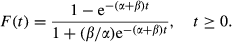
We now proceed to formulate 

Interleaved Sales History
To overcome this difficulty, we will develop a two‐step approximation procedure. In the first step, we will put together a preliminary analysis of sales to potential buyers that does not consider any influencing effect from the interleaved committed‐buyer sales; and then, in the second step, we will make an adjustment to the preliminary analysis that incorporates an incremental sales component which reasonably accounts for the effect of induction from the interleaved sales due to the committed buyers.
We begin with two basic assumptions: From any time epoch t, t ≥ 0, onward, (i) if a potential buyer has not yet made the purchase, then, in the absence of any influence from existing buyers, the distribution of time to purchase for that potential buyer is exponential with rate α; and (ii) if a committed or potential buyer has already made the purchase, then the distribution of time to having a “contact” between that buyer and any one of the remaining potential buyers, and thereby inducing a sale if the latter has not yet made the purchase, is exponential with rate β/(m − 1), where m = 88,000,000. It is important to note that the apportionment of β here is based on the entire market ceiling m, and not just 

A careful reflection on these two assumptions suggests that, with m given, we can take the viewpoint that the rates α and β are the defining attributes of every potential buyer. In the same vein, we can also view 
Denote by 


We hasten to point out that as given in (7), 


We also note that the ratio 


The proof of the claim is essentially the same as that for (26) and (27) in Niu (2006). An adaptation is provided here for completeness. At the beginning of period 1, we have 


Now, for t ≥ 0, define 


The aim of the second step of our analysis is to make an upward adjustment to (8) that takes into account the impact of the dynamic influence from successive purchases made by the committed buyers.
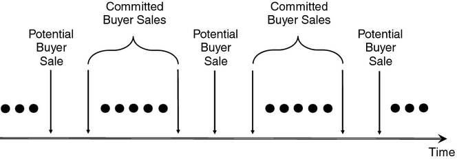
Observe (see Figure 4) that between every pair of consecutive purchases by potential buyers, we have a random number of purchases made by committed buyers. It is stipulated in assumption (ii) that a committed buyer will begin to contribute an induction force of magnitude β/(m − 1) on each member of the potential‐buyer population as soon as that buyer makes the purchase. This has so far been ignored in the preliminary estimate (8). We will now propose a remedy.
Recall that the mean number of committed‐buyer purchases in period 1 is given by 


Conceptually, successive contributions made by the committed buyers to the induction force on the potential buyers should accrue sequentially over time, one by one. An analysis at this level of detail appears to be intractable. The key approximation in our remedy is that we will lump all committed‐buyer purchases between a pair of consecutive (hypothetical) purchases in 
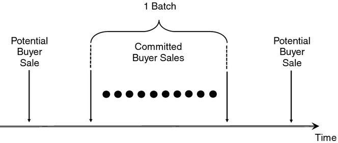
Batching of Committed‐Buyer Sales
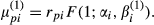
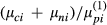
Now, according to the formulation of 


It is interesting to note that although 

We now go beyond period 1 and consider an arbitrary period i, i ≥ 2. We will continue to model sales in a period based on the SBM. However, with i ≥ 2, there would exist an existing sales history at the beginning of period i. Therefore, we need to develop a scheme that dynamically updates the specifications of the successive SBMs to properly reflect any given “expected history” (Niu 2006, p. 686, section 3.2).
We begin with the formulation of the networking effect. Our inclusion of a networking effect in the model is motivated by the fact that sales to the committed and the potential buyers in a period could have a stronger near‐term impact on some members (e.g., those in the same social group) of the residual potential‐buyer population than the force already built into the induction rate β. This naturally suggests that we allow the sales component 


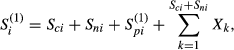
Next, we consider 


Paralleling 


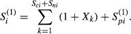
With 


Observe that at the start of period i, the expected total number of existing purchases is given by 


Denote the rate in (13) by 


The rest of the analysis for period i is similar to that for period 1. The only remaining difference is that we now have a networking effect. We will therefore be brief.
For t ≥ 0, define 


To determine a reasonable boost to (15), we will make the additional assumption that the cumulative number of purchases in period i that are due to the networking effect is governed by an independent Poisson process at rate 


Finally, for t ≥ 0, let 
In this subsection, we will develop a recursive scheme that yields a set of approximations for the 
Recall that the total sales 


We begin with the observation that, as 


Under this construction, if we define 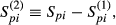


We will next decompose 


With the decomposition of 
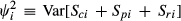
To compute the variance of 


As the variance of a Poisson random variable is equal to its mean, the Poisson assumption above allows us to calculate the variance of the approximation in (23) in terms of the known means. This calculation is now straightforward, and is worked out in section B of Online Appendix S1. The result is: 


It is perhaps interesting to observe that if 


Model Summary
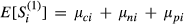
We now provide a summary of the Networking Model. In this model, it is assumed that sales in successive time periods are given by the heteroscedastic nonlinear regression equation defined in (1). The mean 

To compute the means in (1), we decomposed 


An important aspect of the accelerated SBM is that the intrinsic purchase rate 

To compute the standard deviations in (1), we proposed a Poisson approximation for the total sales in each period, given in (23), and used this approximation to estimate the variance of the total sales, which is given in (25). A desirable feature of the estimates for the 
With m set exogenously, the full specification of our model requires seven parameters, namely 


The Re‐Rent Model
We now move on to the formulation of the Re‐Rent Model. The structure of this model is basically the same as that of the Networking Model. Therefore, we will mainly discuss features that are either new or different, and our discussion will be brief.
The Re‐Rent Model is developed here for game rental products. Specifically, for each time period i, we assume that the total sales is given by the sum 


The market ceiling for a game product is denoted by m. Unlike DVD movie products, which have a common market ceiling, the value of m now depends on the game hardware. For each hardware platform, we will set m according to the total number of console units for that platform. The sizes of different platforms are listed in Table 1. The listed values came from the website of PVC Gaming News and Reviews (
There are two reasons for not aggregating game rentals across all platforms. The first is that certain titles may be released only on specific gaming platforms; and the second is that some gaming platforms are more advanced, and therefore elicit different renter behavior (such as a higher degree of product fanaticism) than others.
Apart from setting m differently, the formulation and analysis of the committed‐buyer population is the same as that for the Networking Model. Therefore, the recursion for 
For the potential‐buyer population, there are, however, a few necessary modifications in the formulation. All of the modifications are due to the reasonable assertion (which we make) that a repeat rental by a renter will not generate any incremental influence beyond the induction force that has already been activated by that renter at the time of the first rental.
Consider period i, i ≥ 1. We will assume that a fraction η of the renters counted in 

Next, observe that in contrast to the Networking Model, where each purchase due to the networking effect comes from a new potential buyer (i.e., one who has not yet made a purchase), the re‐rents in the model here, by definition, do not draw from the residual potential‐buyer population. It follows that (12) and (14) should be modified to 


Note that apart from boosting the total expected sales 

We now consider the 


An Empirical Study
The core of our empirical study is a thorough analysis of 352 product titles (170 DVD rental titles, 98 DVD retail titles, 69 game rental titles, and 15 game retail titles), using the models developed in section 3. All of these titles are new products released in the 10‐week time frame from April 2, 2007, through June 9, 2007. The actual sales data were collected from the Blockbuster order management system for the US operations.
An important goal of our empirical work was to test the Networking and the Re‐Rent models against the available data sets, while the models were still under development. The benefit of this approach is that it allowed us to benchmark the validity of various proposed features of the models. For this iterative calibration, we utilized version 7.1 of the
To make parameter predictions for other product titles, we collected a set of “environmental” data that we believe should have a reasonable impact on product sales. Environmental data for DVD movie products (e.g., theatrical sales, MPAA rating, etc.) were obtained from the website 2007; and environmental data for game products (e.g., ESRB rating, genre, replayability rating, etc.) were obtained from the website 2007 Using the collected environmental data and the fitted parameters for the entire set of 352 test titles, we next developed a suite of regression equations (with the environmental information as independent variables) that are individually designed for each parameter (the dependent variable) in our models. The econometric modeling package
Finally, to improve the performance of our forecasts, we further developed a method that makes an adjustment to the initial predictions based on the actual first‐period sales. We believe that the resulting procedure should be of interest to industry practitioners, as it could offer improved ordering or replenishment decisions.
The remainder of this section is organized as follows. In section 4.1, we describe the parameter‐fitting procedure in detail; in section 4.2, we discuss the regression models that are used to make reasonable initial predictions of parameter values for new products; and in section 4.3, we present a method that significantly improves the initial forecasts using actual first‐period sales.
Fitting Parameters
As mentioned above, both the
Our approach is to first use the
As we have 352 different products, it is natural to expect that there would exist many different types of sales trajectories. Therefore, we opted to first perform our iterative model development on a smaller subset of 12 test titles. This test set was chosen because the sales characteristics of these titles covered a diverse range of patterns. The rationale is that if our models are calibrated against this test set, then the resulting models would have a good chance of performing well for the remaining products. This turns out to be true, and in fact, some aspects of our model formulation were actually motivated by the patterns observed in this set of test titles.
The fitted parameters and their standard errors for the titles in the test set are given in Table 2. For most titles, the asymptotic standard errors, which are shown in parentheses below the fitted parameters, are quite reasonable. Note that in a few cases, the fitted values of β, ν, and η are given as 0.000000. This suggests that the induction rate, the networking effect, or the re‐rent effect, respectively, did not play a significant role in the sales for these products.
Fitted Parameters for the 12 Test Titles
Fitted Parameters for the 12 Test Titles


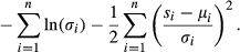
The fit statistics for each of the 12 test titles are provided in Table 3. It can be seen that the 
Fit Statistics for the 12 Test Titles


We now summarize the results for the entire set of 352 titles. First and foremost, we found that overall, the 


As discussed at the beginning of section 3 (see Figure 3, in particular), the key feature in our models is a decomposition of the total sales into three components. To see how the sales components work together effectively to cover a diverse range of sales patterns, we next present the detailed model fits for two examples, one for the Networking Model and the other for the Re‐Rent Model. We also provide three additional examples in section D.1 of Online Appendix S1.
Our first example is “Aurora Borealis.” This is a DVD rental, and hence the Networking Model is used. The fitted sales are plotted in Figure 7. It can be seen that the sales trajectory exhibits a second‐period spike, which is followed by a rapid decay, and then a slight late‐period increase. This is clearly a very challenging trajectory. Nevertheless, our model produced an 
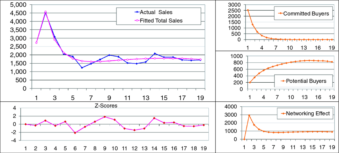
Aurora Borealis
In Figure 8, the fitted sales for our second example, “XBox 360 Forza Motorsport 2,” is plotted. This is a game rental, and hence the Re‐Rent Model is used. The sales trajectory of this game exhibits a sharp drop from the first to the second period, and this is followed by a nearly linear decay pattern. Despite the peculiarity of this trajectory, our model managed to produce an 
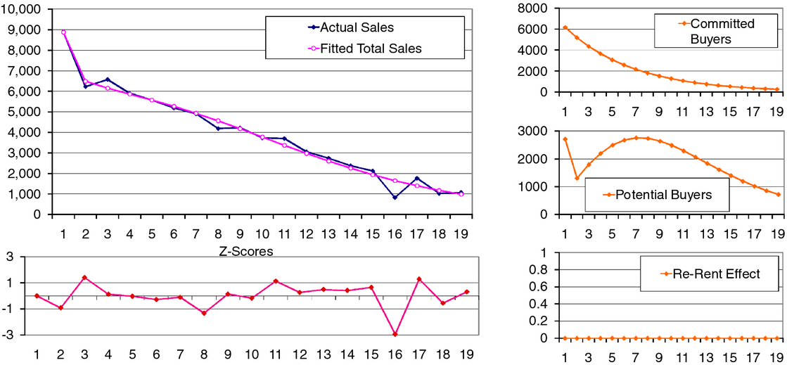
XBox 360 Forza Motorsport 2
These two detailed examples (together with the ones in Online Appendix S1) clearly indicate that our models are capable of offering an improved understanding of the sources of variability in the sales trajectories of these short‐life‐cycle products.
We next report a number of empirical facts regarding the fitted parameters for all 352 data sets. The parameter 


Finally, we comment on the relative strengths of different parameters. The parameters 


As discussed in section 4.1, the Networking and the Re‐Rent Models have been shown to be capable and robust enough to describe the DVD and game sales in the Blockbuster environment. In particular, the sales trajectory for each of the 352 titles has been characterized by a set of seven parameters; that is, for any given set of parameters, the successive expected total sales of a title can be explicitly computed via the recursions developed in section 3. Our goal now is to estimate, for a given new product, these seven parameters prior to any sales activity, based solely on environmental data. For this purpose, we used the parameter characterizations to develop a set of regression equations that, depending on the product type (e.g., movies or games), relate each of the parameters to an appropriate set of environmental variables. Our approach in developing these regressions involved three basic steps, which we summarize next.
First, for each product category, we conducted a correlation analysis, using the fitted parameters for titles in that category, to determine which environmental variables are likely to have a reasonable impact on the parameter values. In our correlation analysis, we also examined how strongly the variables in any proposed set of environmental variables are related to each other; and this was helpful in avoiding possible multi‐collinearity issues.
Second, for each of the parameters, we excluded from consideration all titles with a “low” significance level for that parameter. Our specific criterion is that if the p‐value for a fitted parameter of a title is higher than 0.05, then that title is not used in the analysis for that parameter. Note that this implies that a particular title could be used in the analysis of some of the parameters, but is excluded from the analysis of the other parameters. This is not unreasonable as an insignificant parameter is not expected to have a substantial impact on the values of the remaining fitted parameters.
Lastly, for each parameter, we carefully experimented with various functional forms for the regression equation, using the fitted values from the selected subset of titles, until one with reasonable fit is found for that parameter.
As DVD movie rental is of primary interest at Blockbuster, we will discuss in the remainder of this section results for this product category only (based on the Networking Model).
For movie rental, we identified, after much effort, nine environmental variables that seemed to be most relevant in predicting parameters. These are: (i) four‐week gross theatrical sales, (ii) presence of significant awards, (iii) large studio, (iv) medium studio, (v) large genre appeal, (vi) medium genre appeal, (vii) MPAA rating of UNRATED, (viii) MPAA rating of R, and (ix) MPAA rating of PG‐13. Except for four‐week gross theatrical sales, which is a numeric variable, all other variables in this list are non‐numeric, and are therefore formulated as indicator variables.
In the interest of brevity, we will now further limit our discussion to the parameter 
Our starting point is the belief that the extent of consumer awareness of a movie title should have an influence on the size of the committed‐buyer population. Moreover, it seems reasonable to expect that the 4‐week gross theatrical sales of a movie, which we denote by y, serve as a good proxy for consumer awareness. Indeed, we found a strong positive correlation between 


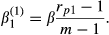
Motivated by the further belief that as the only numeric variable, ln (y) would offer a stronger differentiating power than the other environmental variables, our strategy for constructing the regression for 

Our specific choice of the functional form in the backbone relation is 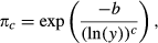


Predicted

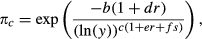
To improve upon (34), we implemented a multiplicative adjustment to each of the shape parameters b and c using two additional environmental variables, large studios and the presence of significant awards (both of which are indicator variables). These two environmental variables, which we shall denote by r and s, respectively, were selected due to a combination of the extents of their correlations with 

Finally, to assess the performance of (35), we used the environmental data alone to predict the 


Using the regression models developed in section 4.2 and in section D.2 of Online Appendix S1, we are now able to forecast sales for a DVD movie title prior to its release, based solely on publicly available environmental data. To assess the performance of our method, we selected a new test set of 11 movie titles and conducted sales forecasts. The titles in this test set are chosen randomly from new releases during the weeks of July 16, 2007 and July 23, 2007; thus, they have not previously been used in any way in our model development.
The performance statistics of our sales forecasts for these 11 titles (based on environmental data) are given in Table 4 under the section heading “Initial Forecast Statistics” (the section labeled “Adjusted Forecast Statistics” will be discussed later in this subsection). The reported statistics are mean absolute deviation (MAD), mean absolute percent deviation (MAPD), and mean squared error (MSE). Of these standard statistics, MAPD is most informative, as it is scaled by the size of the sales volume of a title. It can be seen that our sales forecasts are reasonable for some titles (e.g., an MAPD of 21.87% for “The Number 23”), but are poor for several titles (e.g., an MAPD of 225.81% for “Avenue Montaigne”). Note that we are unable to compare the forecast accuracy of our approach against that of the method employed at Blockbuster as their method is proprietary.
Forecast Statistics for Test Data Set
Forecast Statistics for Test Data Set


Given that our sales model is solidly supported by the empirical results in section 4.1, the performance of the initial sales forecasts should be viewed as a reflection of the predictive power of the environmental variables. In general, if for example, data on product preorders (see, e.g., Moe and Fader 2002, Hui et al. 2008), which has higher power than the environmental data that we have used, were available, it could have been used to improve our forecasts. As such data are not available, we will develop in the remainder of this subsection a procedure that adjusts the initial forecasts based on the actual first‐period sales. The use of first‐period sales allows us to reasonably gauge the “best‐case” performance of our forecasting scheme, in the sense that this is similar to having preorder information.
As noted in section 4.2, the environmental variable y has the strongest correlation with 


We begin with the adjustment for β. From section D.2.4 of Online Appendix S1, the backbone regression equation for β is 
To adjust the predictions for 


The performance of the adjusted sales forecasts for all 11 test titles is reported in Table 4, under the section heading “Adjusted Forecast Statistics.” It can be seen that the MAPDs improved uniformly. The dramatic reduction in the MAPDs for “The Host” and “Avenue Montaigne” is particularly noteworthy.
Finally, we illustrate the forecast adjustments for two of the test titles, “Premonition” and “Factory Girl.” Corresponding results for the remaining nine titles are provided in section D.3 of Online Appendix S1.
Forecasting results for “Premonition” are plotted in 11. The initial sales forecast matches the actual sales trajectory reasonably well. However, the forecast has a slight sales spike in the second period, which is absent in the actual sales trajectory. The spike is removed in the adjusted sales forecast, and this can be attributed primarily to the adjustment in the predicted β.
Sales Forecasts for “Premonition"
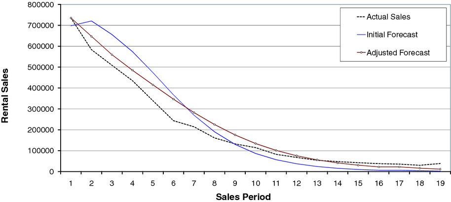
The sales forecasts for “Factory Girl” is shown in Figure 12. The initial sales forecast for the first period, in this case, is substantially lower (over 50,000) than the actual sales for that period. Moreover, the sales forecast is almost linear between periods one and fourteen, which is dramatically different from the actual sales. The trajectory of the adjusted sales forecast is seen to offer significant improvements both in magnitude and in shape. Thus, all three adjustments to the initial predictions for 

Sales Forecasts for “Factory Girl"
In this subsection, we outline the potential benefits of improved forecasts on Blockbuster's retail operations. We will first describe the forecasting method currently in use at Blockbuster, and then illustrate its potential financial impact.
The prevalent forecasting tools at Blockbuster, and this industry in general, are typically confined to rudimentary heuristic methods that are dependent on both historical analogies and personal expertise. At Blockbuster, the management adopts an approach that, similar to the Delphi method, uses a combination of theatrical performance, recent performance of like titles, and the existence of competing titles. This forecasting method is more of an art than a science. Consequently, the results are typically not reproducible and have an inherent degree of error, which is often significant. Therefore, to avoid lost sales, most companies in this industry prefer to err on the side of having inventories that are higher than their sales projections.
The extent of over‐stocking (which is due to a lack of confidence in the forecasting method) at Blockbuster can be illustrated by the set of sample products listed in Table 5. Observe that stocking levels for these products are typically higher than first‐week demands. This is particularly alarming for rental products, as they can be rented multiple times in a week. Moreover, these discrepancies vary dramatically. For rental products, in one instance, the quantity purchased for consumer rentals is as high as three times what was rented; and for retail products, in one instance, the quantity purchased for sales to customers is 26 times what was sold in the first week.
Sample of Rental and Retail Products
Sample of Rental and Retail Products
The cost of over‐stocking can be roughly estimated as follows. For retail products, the average product cost is about $15. If we assume that there are 20 new titles per week for 52 weeks in a year, and that the average size of over‐stocking is 250 pieces per title (conservatively assuming only 1000 pieces purchased and 25% over‐stocking), then product costs for over‐stocking would exceed $4 million annually. For rental products, we can extrapolate from the six titles in Table 5. If we assume that the ideal scenario is for all stores to have sufficient products to meet 100% of first week sales, and that there are 1.3 rents per week per copy (which comes from historical data), then, against this ideal scenario, the company would end up with an average excess of 3108 pieces per title. Now, with about 35 new titles per week for 52 weeks, and still assuming a product cost of $15 per piece, this equates to about $84 million annually.
These cost estimates indicate that there exists significant opportunities for cost reduction in Blockbuster's retail operations (a similar estimate can be made to show significant revenue loss due to under‐stocking). Our method clearly has the potential to enhance revenue and reduce cost for Blockbuster. For example, after an initial order (which could be based on a combination of both our initial forecast and expert opinion at Blockbuster) is placed, our adjusted forecast, which takes into account the actual first‐period sales can be used to revise the ordering decision for subsequent periods. That is, our method can help the operations manager to quickly respond to any mismatch in the initial order, and thereby improve the net profit for the remainder of the life cycle of a product.
In this article, we have used the actual sales history of 352 different new product releases from Blockbuster to develop and test two versions of a sales model. Our model integrates: (i) multiple consumer sub‐populations, (ii) cross interactions between the sub‐populations, and (iii) dynamic updates, both within and across time periods, for the purchase rates of the consumers in the sub‐populations.
Using publicly available environmental data and actual first‐period sales, we demonstrated that the model is capable of delivering reliable sales forecasts for DVD movie rental. We also discussed the potential for the model to make a significant financial impact on Blockbuster's retail operations.
The key feature in our sales model, namely the demand decomposition exhibited in Figure 3, is by no means particular to just new product releases at Blockbuster. This modeling approach, which we believe is a useful contribution of this article, can be adapted to suit other short‐ (and possibly long‐) life‐cycle products. The formulation can also be integrated into other models for operational decisions (see, e.g., Bassamboo et al. 2009, Debo et al. 2006, Ho et al. 2002, Kumar and Swaminathan 2003). We are currently pursuing further research in such models in the context of online movie rental operations.
Our work suggests two possible managerial implications. The sales decomposition suggests that managers could try to “conceptually” manipulate the relative sizes of different market segments. For example, even though explicit identifications of the segments are not possible, in‐store or online advertising could be used in an attempt to boost the size of the committed‐buyer population. The sales trajectory of a product can be expected to have lower variability if the size of this population is relatively larger.
Our sales model has been shown to be accurate (see Figure 6). The performance of sales forecasts based on our model, however, will further depend on the availability of quality input data. This suggests that Blockbuster could narrow down its forecasting effort to that of building reliable methods for predicting model parameters. In this article, the sales forecasts (see section 4.3) are based on environmental information. In general, if independent forecasts from in‐house experts and/or preorder or other relevant data are available, they could be built into the parameter‐prediction models to produce improved forecasts.
Finally, we note that we did not consider the effects of price and advertising in our formulation. This is due to the fact that product offerings at Blockbuster typically have a fixed price, and that Blockbuster relies primarily on studio advertising (which can be taken as a form of environmental information). These effects could have significant impacts on the sales trajectory of products in other arenas, and are therefore worthy of further study.