
Abstract
Due to the growing concern over environmental issues, regardless of whether companies are going to voluntarily incorporate green policies in practice, or will be forced to do so in the context of new legislation, change is foreseen in the future of transportation management. Assigning and scheduling vehicles to service a pre‐determined set of clients is a common distribution problem. Accounting for time‐dependent travel times between customers, we present a model that considers travel time, fuel, and CO2 emissions costs. Specifically, we propose a framework for modeling CO2 emissions in a time‐dependent vehicle routing context. The model is solved via a tabu search procedure. As the amount of CO2 emissions is correlated with vehicle speed, our model considers limiting vehicle speed as part of the optimization. The emissions per kilometer as a function of speed are minimized at a unique speed. However, we show that in a time‐dependent environment this speed is sub‐optimal in terms of total emissions. This occurs if vehicles are able to avoid running into congestion periods where they incur high emissions. Clearly, considering this trade‐off in the vehicle routing problem has great practical potential. In the same line, we construct bounds on the total amount of emissions to be saved by making use of the standard VRP solutions. As fuel consumption is correlated with CO2 emissions, we show that reducing emissions leads to reducing costs. For a number of experimental settings, we show that limiting vehicle speeds is desired from a total cost perspective. This namely stems from the trade‐off between fuel and travel time costs.
Introduction
The ever‐growing concern over greenhouse gases (GHG) has led many countries to take policy actions aiming at emissions reductions. Most notable is the Kyoto Protocol, which requires countries to reduce a basket of the six major GHG by the year 2012 by 5.2% on average (compared to their 1990 emission levels). Next to this, a number of other initiatives have emerged particularly to control CO2 emissions. For example, more than 12,000 industrial plants in the EU are subjected to CO2 caps, enabling the trade of emissions rights between parties. For a comprehensive survey of GHG trade market models, the reader is referred to Springer (2004).
The importance of environmental issues is continuously translated into regulations, which potentially have a tangible impact on supply chain management. As a consequence, there has been an increasing amount of research on the intersection between logistics and environmental factors. Sbihi and Eglese (2007) identified potential combinatorial optimization problems where Green Logistics is relevant. Corbett and Kleindorfer (2001,2001) discussed the integration of environmental management in operations management. Kleindorfer et al. (2001) did so in the context of sustainable operations management. Lee and Klassen (2008) mapped factors that initiated and improved environmental capabilities in small‐ and medium‐sized enterprises over time.
European road freight transport uses considerable amounts of energy (Baumgartner et al. 2008). Vanek and Campbell (1999) note that predictions are that the United Kingdom will meet the Kyoto targets. However, they highlight that within the period from 1985 until 1995, energy use across all sectors grew only by 7% while transport energy use grew by 31%. Similar findings were observed by Léonardi and Baumgartner (2004). They state that in the period 1991–2001 road freight traffic in Germany increased by 40%. Moreover, in 2001 traffic was responsible for about 6% of total CO2 emissions in Germany. More substantial CO2 increases are observed in India by Singha et al. (2004), where the CO2 emissions from road transport in the year 2000 have increased by almost 400% compared to 1985. In the context of examining scenarios for GHG, Yang et al. (2008) mention that in California the transportation sector accounted for over 40% of GHG for 2006, making it by far the largest contributor. Baumgartner et al. (2008) acknowledge that new vehicle designs are more efficient in terms of emissions. However, this is outweighed by the transport growth rate in the EU. Ericsson et al. (2006) mention that CO2, which is directly related to the consumption of carbon‐based fuel, is regarded as one of the most serious threats to the environment through the greenhouse effect. Globally, transportation accounts for about 21% of CO2 emissions. In the same spirit, CO2 is identified as the most important greenhouse gas in the Netherlands, as it accounted for 80% of total emissions in 1995 (see e.g., Kramer et al. 1999). Thus, there is a clear necessity to control CO2 emissions.
Road transport accounts for a large portion of CO2 emissions, of which goods transport constitutes a sizeable portion. Thus, there is a need to address environmental concerns in the context of goods transport. Carrier companies may voluntarily adopt green policies if this is aligned with profitability. This could be in the form of GHG trading mechanisms, or when CO2 becomes a taxable commodity. Another reason for adopting green policies is the marketing potential of a greener company image, for example, controlling the carbon footprint. Furthermore, new regulations might force companies to change practices. It is worth mentioning that the department for environment, food and rural affairs in the United Kingdom values the social cost of carbon between £ 35 and £ 140 per tonne. In essence, pricing carbon emissions leads to an assessment of its economic impact and regulations might be formed accordingly. In conclusion, either for exogenous or endogenous reasons, change is anticipated in transportation management because of environmental factors. We argue that logistics service providers should contemplate how to deal with these issues.
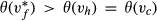
The focus of this article is on incorporating CO2‐related considerations in road freight distribution, specifically in the framework of the Vehicle Routing Problem (VRP). CO2 emissions and fuel consumption both depend on the vehicle speed, which changes throughout the day due to congestion. Thus, it is relevant to study the problem in conjunction with time‐dependent travel times, i.e., where the travel time depends on the time of day at which a distance is traversed. Time‐dependency is modeled by partitioning the planing horizon into free flow speed periods and periods with congestion, that is, lower speeds. We introduce a new variant of the VRP that accounts for travel time, fuel, and CO2 emissions costs. This results in the Emissions‐based Time‐Dependent Vehicle Routing Problem, denoted by E‐TDVRP. The E‐TDVRP builds on the possibility that carrier companies limit the speed of their vehicles. Thus, the vehicle speed limit is explicitly part of the optimization. The traditional Time‐Dependent Vehicle Routing Problem (TDVRP) optimizes exclusively on travel times and does not consider limiting vehicle speed. However, we show that when accounting for fuel, travel time, and emissions, controlling vehicle speed is desirable from a total cost point of view.
The E‐TDVRP is clearly a complex problem, as in addition to the complexity of the TDVRP, it also determines the free flow speed. This implies that one needs to allocate customers to vehicles, determine the exact order in which customers are visited, and set the free flow speed. The free flow speed impacts the resulting travel time function of each arc, and in return, affects the moment vehicles go into congestion. We assume that the congestion speed remains constant, as it is imposed by traffic conditions. This leads to a situation where speeds can be controlled in particular time periods of the day, that is exclusively in free flow periods. The E‐TDVRP can be reduced to two sub‐problems: one where only the CO2 emissions are taken into account in the optimization (that is, a pure environmental model) and one where only travel times are considered (i.e., a pure logistical cost model). As such, we study the trade‐off between minimizing CO2 emissions as opposed to minimizing total travel times. In addition, we develop bounds for the potential reduction in CO2 emissions. These bounds are based on solutions of the standard time‐independent VRP. Since most optimization tools used in industry consider time‐independent travel times, such bounds can concretely aid decision makers in evaluating the maximum reduction in emissions.
The remainder of the article is organized as follows, Section 2 reviews the relevant literature. Section 3 describes the E‐TDVRP model. It also introduces bounds for the potential savings in CO2 emissions. The solution method is discussed in section 4 The experimental settings and results are presented in section 5 Finally, section 6 highlights the main findings and indicates directions for future research.
Literature Review
Van Woensel et al. (2001) highlighted the value of traffic flow information in relation to emissions. Their results showed that calculating emissions under constant speed assumptions can be misleading, with differences of up to 20% in CO2 emissions on an average day for gasoline vehicles and 11% for diesel vehicles. During congested periods of the day these differences rose 40%. Similar results were shown by Palmer (2008), for a number of roads. Such results are motivated mainly by the fact that CO2 emissions are proportional to fuel consumption (Kirby et al. 2000), and thus are speed dependent. The relation between emissions and vehicle speed leads to the study of the VRP problem in a time‐dependent framework. In what follows, we first discuss the literature concerning the TDVRP, and then review the literature dealing with routing and emissions.
Assigning and scheduling vehicles with a limited capacity to service a set of clients with known demand, is a problem faced by numerous carrier companies. It has been extensively researched in the literature as the well‐known VRP. For a comprehensive review, the reader is referred to Laporte (2007). In its most standard version, the problem deals with minimizing costs subject to demand satisfaction and vehicle capacity constraints. Each customer is visited by a single vehicle, each vehicle starts and ends its route at the depot. The relevance of the VRP to real‐life practice coupled with the hard nature of the problem has attracted much research. To model reality more accurately, numerous features have been added to the problem. One of these is including speed changes over the day, in an attempt to account for traffic congestion experienced in certain periods of the day.
Lately, a number of researchers incorporated time‐dependent travel times between customers into the VRP, which gave rise to the TDVRP. The objective of the TDVRP, in most cases, is similar to that of the VRP, that is, minimizing costs (Hill and Benton 1992). However, in the TDVRP the travel time cost depends on the time of day a distance is traversed. Modeling time‐dependency is mostly done by associating different speeds to a number of time zones within the planning horizon. Malandraki and Daskin (1992) motivate variability in travel time by random events, such as accidents and cyclic temporal variations in traffic flow. They propose a mixed integer programming formulation for the TDVRP. Malandraki and Dial (1996) propose a dynamic programming formulation to solve the time‐dependent Traveling Salesman Problem (TSP). However, both these articles modeled travel times by discrete step functions where travel times are associated with different time zones. Although this modeling approach does capture variability in travel times, it enables the undesired effect of surpassing. This effect implies that a vehicle departing at a certain time might surpass another vehicle that started traveling earlier. This limitation was discussed by Fleischmann et al. (2004), Ichoua et al. (2003), Nannicini et al. (2010), and Van Woensel et al. (2008). All these articles model time‐dependencies complying with the First‐In First‐Out (FIFO) assumption, which does not allow for surpassing. This is done by using appropriate piecewise linear functions for travel times. In this article, we adopt travel time functions similar to the ones used by Ichoua et al. (2003), and thus adhere to the FIFO assumption.
Ichoua et al. (2003) modeled the TDVRP by partitioning the day into three speed zones, where the speed differences due to congestion were determined by different factors of the free flow speeds. The travel time profiles were constructed by piecewise linear functions. Fleischmann et al. (2004) discuss a general framework for integrating time‐dependent travel times in a number of VRP algorithms. Furthermore, they provide an overview of traffic information systems from which data can be collected. Modeling of time‐dependent travel times would benefit from these data. Based on empirical traffic data, queueing models were developed by Van Woensel (2003) to model congestion, where the model parameters were set to incorporate different traffic flows and weather conditions. The analysis of the data resulted in average speeds for different time zones (see also Van Woensel and Vandaele 2006). These speeds were later used in Van Woensel et al. (2008) to solve the TDVRP with tabu search. Jung and Haghani (2001) proposed a modified genetic algorithm to solve the TDVRP.
Not much research has been conducted on the VRP under minimizing emissions. Cairns (1999) studied the environmental impact of grocery home delivery, but this was done by converting distance into emissions, irrespective of speed changes. The effect of speed changes is incorporated in the work of Palmer (2008). He studied emissions in the context of grocery home delivery vehicles, where real traffic data were used to derive fuel consumption and emissions. A similar detailed methodology was used by Ericsson et al. (2006). Both Palmer (2008) and Ericsson et al. (2006) considered CO2 minimization as an optimization criteria. Bektaş and Laporte (2011) introduced the pollution routing problem where they accounted for the amount of greenhouse emissions, fuel, travel times, and their costs. The authors present a comprehensive formulation of the problem and solve moderately sized instances. Scott et al. (2010) investigated the influence of the minimization of CO2 emissions on the solutions to shortest path and traveling salesman problems in freight delivery applications. Real life examples are studied using the road network of Scotland. In a more aggregate view, Sugawara and Niemeier (2002) presented an emissions‐based trip assignment optimization model. They also explored potential emission reduction under the assumption that drivers choose emission minimizing routes. Assessing vehicle emissions can be very complex, as emissions depend on factors such as the age of the vehicle, engine state, engine size, speed, type of fuel, and weight (Taniguchi et al. 2001). For our study, we use speed emission functions from the MEET model (European Commission 1999). In this article, we focus on CO2 and leave other pollutants for additional research.
Description of E‐TDVRP
This section starts with a complete description of the E‐TDVRP model and details the most relevant parts of this model. Section 3.1 elaborates on the computation of the travel times. Section 3.2 explains the computation of the CO2 emissions and fuel consumptions. Finally, in section 3.3 the bounds on CO2 emissions are presented.
In general, the VRP is described by a complete directed graph G = (V,A) where V = {0,1,…,n} is a set of vertices and A = {(i,j):i<>j ∈ V} is the set of directed arcs. The vertex 0 denotes the depot; the rest of the vertices represent customers. For each customer, a non‐negative demand


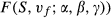
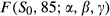
The E‐TDVRP differs from the VRP as it considers time‐dependent travel times. Furthermore, it considers fuel and emissions costs. The objective function of the E‐TDVRP is the sum of all these costs. Limiting the free flow speed of the vehicles is examined in this problem. Therefore, in addition to the routing solution the E‐TDVRP has a decision variable


We define a solution as a set S with s routes


A solution (


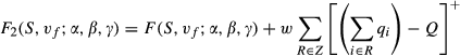
We define three cost factors in the E‐TDVRP: the hourly cost of a driver (with a cost of α €/hour), the cost of fuel (costing β €/liter), and the cost of CO2 emissions (γ €/kg). Since fuel consumption is directly related to CO2 emission, we use the factor of h (equal to


The first part of the objective function considers the travel time costs. The second part considers the composite costs combining fuel and emissions. We explicitly consider both, as the cost parameters for fuel (β) and emissions (γ) are different.
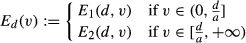
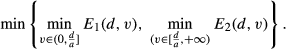
The E‐TDVRP can be reduced into two special cases. Setting α to zero the model minimizes solely the costs of fuel and CO2, which is equivalent to minimizing


For completeness, we summarize the speed‐related notation we will use in the remainder of this section:


Determining

The time‐dependency of travel times throughout the planning horizon, is in essence, driven by changing speeds in different time zones. We subject all links to given speed profiles. This stems from the notion that most motorways, on average, follow the same pattern of having morning and evening congestion periods (see Ichoua et al. 2003 for a similar reasoning). Moreover, collecting data for each link and each time zone is infeasible from an operational standpoint.
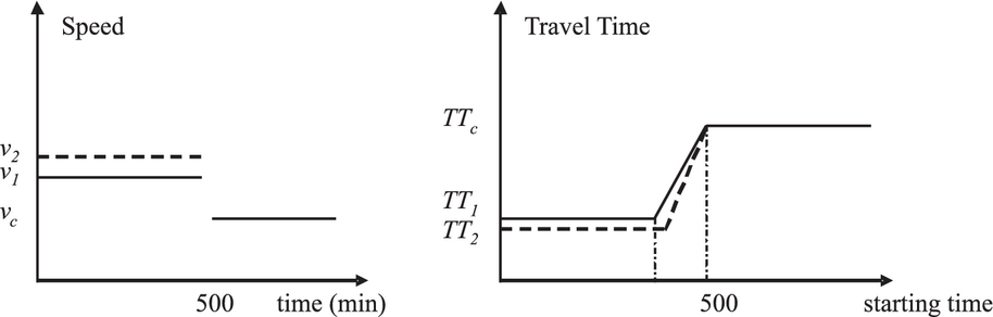
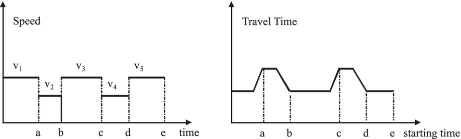
Figure 1 provides an illustration of how speeds are translated into travel time profiles. The left side depicts a speed profile that starts with a congestion speed


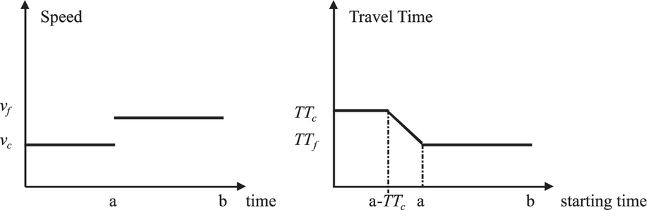
The Conversion of Speed into Travel Times
The linearity in the transient zone stems from the stepwise speed change which imposes different speeds over time. The slope can be defined as


For starting times within


The proposed model is convenient since it requires speed values and the points in time at which the speed changes.


In this article, we use emission functions provided in the MEET report (European Commission 1999). The function θ(v) provides the emissions in grams per kilometer for speed v. Equation (3) depicts the amount of emissions per km, given that a vehicle is at speed v.
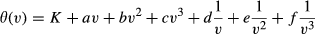
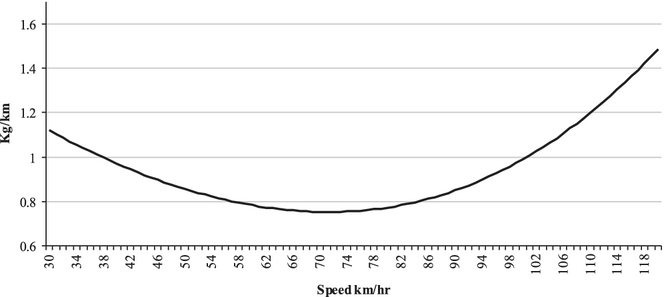
The coefficients (K,a,…,f) differ per vehicle type and size. Here, we focus on heavy duty trucks weighing 32–42 tons. The coefficients for the CO2 emissions for this specific vehicle category are (K,a,b,c,d,e,f) = (1576, −17.6, 0, 0.00117, 0, 36067, 0). Figure 2 depicts this CO2 (kg/km) emissions function. This function has a unique minimum and we define


CO2 Emissions vs. Speed
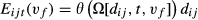
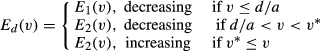
We denote the amount of CO2 emissions in grams produced by traversing arc (i,j) at time t with a free flow speed


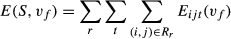
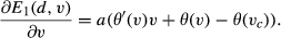
The objective function for term


Both from a practical and an optimization point, we choose to work with integer speeds. Optimizing on


Modifying the speed profile affects the travel time profiles. As explained in section 1, the change of speed at point a starts affecting the travel times already at point


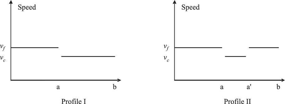
Example for Two Free Flow Speeds
Considering optimizing on


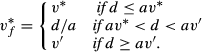
Given


For the case of θ(v) being convex having a unique minimum as is in the case of the CO2 emission function considered, Proposition 1 is straightforward to show. Since


Arguing by contradiction, assume that


As previously mentioned, we only consider integer values for speeds. Thus,


The

The lower bound is realized by traversing the total distance in the VRP solution with a speed

Speed Profiles for the Bounds on E‐TDVRP
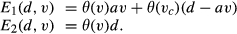
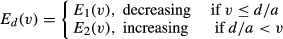
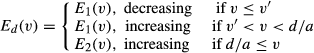
We analyze the case of subjecting the VRP solutions to Profile I. We denote the distance of an arbitrary route by d. We distinguish two cases: If the vehicle is not fast enough to avoid congestion, that is, v < d/a, then the total emissions are given by the emissions in free flow θ(v)av plus the emissions in congestion which are If the vehicle travels fast enough to avoid congestion, that is, v ≥ d/a, then the total emissions would simply be given by θ(v) times the covered distance d.

According to the above distinction, define


Then, total emissions as a function of distance d can be written as a function of speed:
In our case


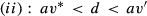
There exists a universal speed


As earlier observed
it is sufficient to put together Case Case Case


The importance of Lemma 1 is that for large enough distances,


Let


The upper bound is constructed by imposing Profile I with


Given the standard VRP solution, these bounds are rather straightforward to calculate, and enable decision makers to easily assess the maximal reduction in CO2 emissions. Furthermore, these bounds are used to validate the proposed solution procedure.
We propose a tabu search procedure for the E‐TDVRP. Tabu search was first introduced by Glover (1989,1989). It makes use of adaptive memory to escape local optima. The method has been extensively used for solving the VRP; see Gendreau et al. (1994,1996 Hertz et al. 2000) for examples. Tabu search is also used to deal with the time‐dependent version of the VRP (see Ichoua et al. 2003, Jabali et al. 2009, Van Woensel et al. 2008). The E‐TDVRP model differs from the TDVRP as it includes the free flow speed


Algorithm 1 E‐TDVRP algorithmic structure
The initial solution 


Similar to Gendreau et al. (1994), we allow capacity‐infeasible solutions, i.e., routes with total demand exceeding the vehicle capacity. Such infeasible solutions are penalized, in proportion to the capacity violation, by the following objective function, extending 
In Equation (8)
(9) each unit of excess demand is penalized by a factor w. This penalty w is decreased by multiplication with a factor ν after ϕ consecutive feasible moves. Similarly, w is increased (multiplied by factor 
Every σ iterations, we consider the best found solution 


Experimental Settings
We conducted two types of experiments. Section 1 describes our experiments with a single speed profile. The other experiments include two speed profiles and are presented in section 2 We experiment with sets from Augerat et al. (1998). The number of nodes in these sets ranges between 32 and 80. To achieve more realistic travel times, the coordinates of these sets were multiplied by 4.9. Note that a test set named “32 k5” means 32 customers including the depot with five vehicles. Optimal VRP solutions for these sets are available from Ralphs (2011).
Single Speed Profile
We set up the speed profile with two congested periods, while throughout the rest of the day the speed is set to the free flow speed (Figure 5, left). Many European roads face such a morning and afternoon congestion period (see Van Woensel and Vandaele 2006). The right side of Figure 5 depicts the travel time function for each starting time for an arbitrary distance. We set 


Speed and Travel Time Profile for the Experimental Setting
Observe that a starting time after 9:00 hours is superior to starting time before 9:00 hours, since the latter risks going twice into congestion. Consequently, we assume that all vehicles leave the depot at 9:00 hours. To compute the upper bound, we set a in Equation (8) to c − b. Considering 


The parameters chosen for the costs and the tabu search algorithm in section 4 are summarized in Table 1. We note that γ is based on the actual carbon market cost of the first half of April 2009 (Point Carbon 2009). All runs are performed on a Intel Core Duo with 2.4 GHz and 2 GB of RAM.
Table 2 shows the results for the reduced model where we focus on emissions, that is, with the objective function 


Cost and Tabu Search Parameter Values
Cost and Tabu Search Parameter Values
We tested the performance of our algorithm on the standard time‐independent VRP from Augerat et al. (1998). The algorithm reached an average optimality gap of 4% over the different sets. Furthermore, we evaluated the performance when setting the free flow speed to 71 km/hour (F(S,71;0,0,1)), which is the speed that minimized the CO2 emissions function as observed in Figure 2. The results showed that adopting this speed leads to an average increase of 2.9% and 6.0% in emissions and travel times, respectively, when compared to the results in Table 2 (see Online Appendix S1 for further details).
Results for the 


To validate the model, we compare the results of 


Upper and Lower Bounds for 


Table 4 gives an overview of the cost‐based solutions for all sets (α = 20 €/hour, β = 1.2 €/l and γ = 11 €/ton). The last three columns give the allocation of costs between its three major components.
Results for

(

) (One Speed Profile)
Results for


The vast majority of costs are attributed to driving cost and fuel cost, which together on average account for 98.6% of the costs. The cost of CO2 is rather insignificant when compared to others: 1.4% on average. Specifically, the current market cost of CO2 has no tangible economic impact on the results. However, due to the direct relation between fuel consumption and CO2, speeds associated with this model are between 80 and 87 km/hour. In fact, in all instances the resulting speed is strictly less than 90 km/hour. This implies that even with the current cost structure speeds are likely to be <90 km/hour.


We analyze the results for the two reduced models. The first one optimizes only on the emissions (
Let 


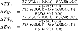
In the above expressions the current situation corresponds to the setting with a fixed speed, that is, 80 or 90 km/hour, where the minimization is on the total travel time. In the alternative situation the objective is to minimize emissions, that is, the objective function 
Table 5 gives an overview of the potential savings in emissions, compared to the amount of travel time needed to be sacrificed to achieve this saving. Columns 2 and 3 exhibit the decrease in emissions, while the last two columns exhibit the increase in emissions. Considering the speed limit of 90 km/hour, Table 5 implies that an average reduction of 11.4% in CO2 emissions can be achieved. However, such a reduction will result in an average increase in travel time by 17.1%. Looking to the situation with a speed limit of 80 km/hour an average of 3.2% reduction in emissions can be achieved, which would require an average increase of 6.6% in travel time. These results show that in the case of 90 km/hour a substantial reduction of CO2 emissions can be achieved.
Trade‐off between Emissions and Travel Times (One Speed Profile)
Trade‐off between Emissions and Travel Times (One Speed Profile)


In this section we consider two speed profiles. In addition to the profile considered in section 1, we add a similar profile but with a congestion speed equal to 70 km/hour similar to (Van Woensel and Vandaele 2006), instead of 50 km/hour. The two profiles were randomly assigned to the various distances in the instances.
We ran 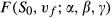
Results for

(Two Speed Profiles)
Results for


Both for the single and for the two speed profile case the resulting speeds (


As the resulting speeds for both one and two speed profiles are within similar ranges, we examine the case where we set 

Table 7 exhibits the results of setting 

Comparison of F(


Carrier companies need to consider employing greener practices in the future. This article establishes a framework for modeling CO2 emissions in a time‐dependent VRP context, by the E‐TDVRP model. It proposes an efficient solution method for the E‐TDVRP. We show the potential reduction in emissions when weighed against travel time. Furthermore, we show that reducing emissions may have a positive impact with respect to reducing cost.
We analyzed the effect of limiting vehicle speed in a time‐dependent VRP setting on the generated amount of CO2 emissions. Time‐dependency was established by subjecting distances to variable speed profiles. CO2 emissions were modeled as a function of speed. The speed, which optimizes CO2 emissions per km, was not observed in any of our experimental settings. This is explained by the relation between limiting free flow speed and the likelihood of running into congestion. In congestion, the vehicle is forced to drive more slowly and emits more CO2. Thus, increasing the free flow speed decreases the amount of time spent in congestion, and thereby may result in less emissions.
Based on the optimal VRP solutions in the literature, we constructed an upper and lower bound for CO2 emissions. We showed that these bounds are tight, on average the gap was 4.7%. From a practical point of view these bounds are simple and fast to calculate. They require standard VRP solutions that are commonly used in practice. The bounds enable the assessment of the potential reduction in CO2 emissions.
Considering CO2 emissions, the results of the E‐TDVRP were rather close to the lower bound, with a difference of 4.3% on average. This indicates that the chosen solution strategy was adequate. We compared two extreme cases of the E‐TDVRP model, considering only travel times and considering only CO2 emissions. For the first case, two possible speed limits were considered, 80 and 90 km/hour. For a speed limit of 90 km/hour our results showed that achieving an average reduction of 11.4% in CO2 emissions required an average increase in travel time of 17.1%. However, for a speed limit of 80 km/hour, an average increase of 6.6% in travel times achieves a reduction of 3.2% in CO2 emissions.
Considering one and two congestion speeds, the experiments showed that from a realistic cost perspective it is beneficial for vehicles to go below 90 km/hour. We also showed that adopting a speed limit of 85 km/hour yields good results in terms of total cost over all sets. Finally, we conclude that minimizing CO2 emissions by limiting vehicle speed can be costly in terms of travel time. Nevertheless, limiting vehicle speed to a certain extent might be both cost and emission effective.
Additional enhancement of the algorithm may facilitate the solution of larger instances. Future research can also focus upon more accurate emissions modeling. For example, the weight of the vehicle has an impact on the amount of emissions, and in the VRP context this can be incorporated as a function of satisfied demand. In addition, more sophisticated travel time profiles can be constructed to encompass acceleration and deceleration, which in return will enable more accurate emissions modeling. Furthermore, the proposed model can be employed to investigate the costs and benefits of using alternative fuels in the context of VRP.
We have shown that the current market cost of CO2 has no tangible economic impact on the results. However, exploring this value is yet another possible extension to this work. Examining the impact of this value on transportation‐related strategies is a relevant research question.
Footnotes
Acknowledgments
The research of Ola Jabali has been funded by the Netherlands Organization for Scientific Research (NWO), project number 400‐05‐185. Thanks are due to the referees for their valuable comments.
