
Abstract
In make‐to‐stock production systems finished goods are produced in anticipation of demand. By contrast, in stockless production systems finished goods are not produced until demand is observed. In this study we investigate the problem of designing a multi‐item manufacturing system, where there is both demand‐ and production‐related uncertainty, so that stockless operation will be optimal for all items. For the problem of interest, we focus on gaining an understanding of the effect of two design variables: (i) manufacturing speed—measured by the average manufacturing rate or, equivalently, the average unit manufacturing time, and (ii) manufacturing consistency—measured by the variation in unit manufacturing times. We establish conditions on these two variables that decision makers can use to design stockless production systems. Managerial implications of the conditions are also discussed.
Introduction
In make‐to‐stock production systems finished goods are produced in anticipation of demand. By contrast, in stockless production systems finished goods are not produced until demand is observed. In this sudy we examine the problem of designing a multi‐item manufacturing system, where there is both demand‐ and production‐related uncertainty, so that stockless operation will be optimal for all items. Note that we use the term stockless in lieu of make‐to‐order as the latter term is sometimes also used to denote the mode of operation where finished goods are manufactured according to customer specifications, which we do not consider herein.
Our interest in the problem of designing stockless production systems grew out of consulting work we performed for firms in two very different industries. One consulting project was done with a manufacturer of commercial airplanes, the other with an oil and gas company. As shall become apparent to the reader, our findings have applicability to firms in a variety of industries. For the problem under study we focus on gaining an understanding of the effect of two variables that are encountered in the design of production systems. One variable considered is manufacturing speed, measured by the average manufacturing rate or, equivalently, by the average unit manufacturing time. The other variable considered is manufacturing consistency, measured by the variation in unit manufacturing times.
Interest in stockless production systems now spans a number of decades with the earliest work on the subject being that of Popp (1965), which looked at the make‐to‐stock versus stockless operation question for a single item. Since then multi‐item manufacturing settings have been investigated. Some recent work includes that of Federgruen and Katalan (1999), where the impact of adding a stockless item to a make‐to‐stock production system was studied, and that of Arreola‐Risa and DeCroix (1998) and Rajagopalan (2002), which explored which items of a collection ought a firm to produce make‐to‐stock and which items are best produced under stockless operation. The work of Rajagopalan assumed a setup time between items while the earlier work of Arreola‐Risa and DeCroix did not. It should also be mentioned that the problem studied in Arreola‐Risa and DeCroix is different from our work in this study in three fundamental ways. First, they focused on determining the stockless condition for one item within a set of items, while we seek conditions under which stockless operation will be optimal for all items. Second, they studied an existing production system where manufacturing speed and consistency were known and fixed, and the decision variables are the values of the base‐stock levels. In contrast, our production system is being designed, and hence the decision variables are the values of manufacturing parameters so that stockless operation is optimal. Third, we model unit manufacturing time as having a continuous phase‐type or a gamma distribution. Arreola‐Risa and DeCroix used different probability distributions to model unit manufacturing time.
Other recent work has primarily examined scheduling‐related issues and includes that of Zheng and Zipkin (1990), Veatch and Wein (1996), de Vericourt et al. (2000), Veatch and de Vericourt (2003), and Youssef et al. (2004). A significant amount of research has also been conducted on assemble‐to‐order systems (see Song and Zipkin 2003), however that research stream lies outside the focus of this work. Lastly, zero‐inventory situations due to product perishability or duopoly competition can be found in Geismar et al. (2011) and Sun et al. (2008), respectively.
We make three major contributions with this article. First, we establish conditions on the design variables manufacturing speed and manufacturing consistency that decision makers can use to design a production system whose operation is optimally stockless for all items. Second, we identify theoretical properties of our findings that may provide guidance to researchers in their study of similar production systems. Third, we discuss several managerial implications of our results that should be of interest to supply chain managers considering a stockless strategy. Of special interest is the dynamic between risk pooling and stockless production.
The article has five more sections. Section 2 describes the problem setting and the model we employ in this study. Section 3 investigates multi‐item systems, while section 4 looks at the single‐item case. Section 5 illustrates the application of our results in a real‐world project. Section 6 presents our conclusions and future research directions.
Problem Setting and Model
We consider a firm that is a manufacturer of several types of finished goods, where the different types of finished goods are called items. Items are manufactured one unit at a time, have setup times and setup costs that are negligible, share the same production facility, and experience manufacturing times that may exhibit variability from unit to unit, which we assume without loss of generality, that is, the special case of deterministic manufacturing times is, not necessarily excluded. The distribution of unit manufacturing times is the same for all items.
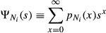
Let M denote unit manufacturing time. To maximize the applicability of our results, we first model M as having a continuous phase‐type (PH) distribution. The continuous PH distribution is dense in the field of all positive‐valued distributions, that is, it can approximate any distribution on the nonnegative reals (see e.g., Kao 1997). Let


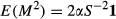
To measure manufacturing speed, we will use the average manufacturing rate, or equivalently, the average unit manufacturing time. Letting μ and E(·) respectively denote the average manufacturing rate and the expected value operator, from Equation we have that
To measure manufacturing consistency, we will use the squared coefficient of variation, which is defined as the ratio of the variance to the mean squared. Letting V(·) and SCV(·) respectively denote the variance and squared coefficient of variation operators, from Equation we have that since

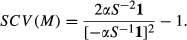
Note that the lower the value of SCV(M), the greater the consistency of unit manufacturing times. Also, because the SCV(·) is a relative measure, it allows for comparison across different manufacturing environments. Although there is no generally accepted standard as to what constitutes a “high” or “low” squared coefficient of variation, a value of < 0.25 is typically viewed as signaling low variability (high manufacturing consistency), while a value > 0.75 is typically viewed as signaling high variability (low manufacturing consistency). See Knott and Sury (1987) for an empirical study that offers further guidance on this subject matter.
It is worth noting that modeling M as having a continuous phase‐type distribution is appealing as it holds with some generality. However, use of continuous phase‐type makes the manipulation of the design variables, that is, manufacturing speed and manufacturing consistency (captured in Equations and , respectively), very challenging. In our consulting work the system designers ultimately decided to model M using the gamma family of distributions. This was done for three reasons: The gamma distribution does not take negative values and manufacturing times were being modeled. The gamma distribution can adopt both symmetric and asymmetric shapes. The gamma distribution allowed for easy manipulation of the design variables.
When M is modeled as distributed according to the gamma family (see e.g., Taylor and Karlin 1998)
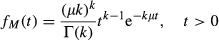
It follows that for the Gamma(μ,k)

Hence the average unit manufacturing time is equal to the reciprocal of the parameter μ, the manufacturing rate or speed, which is one of the design variables of interest. Furthermore, we have that (see e.g., Allen 1990)
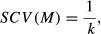
A comparison of Equations and with Equations and makes it clear that the design variables of interest are much easier to manipulate when M has a Gamma(μ,k) distribution than when M has a PH(α,S,k) distribution. The Gamma(μ,k) distribution offers two more advantages that should also be of interest to real‐world system designers.
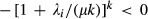
First, Theorem 2 in O'Cinneide (1991) states the following: “The coefficient of variation of an order k PH‐distribution is at least

A second advantage of the Gamma(μ,k) distribution is subtle but very relevant to real‐world system designers. We also know from Theorem 2 in O'Cinneide (1991) that the Erlang distribution minimizes the order k of PH(α,S,k) distributions required to achieve a SCV value, and we know that when k is integer, the gamma distribution becomes an order‐k Erlang distribution. Consequently, if a production system designer wants to model M as a PH(α,S,k) distribution, and at the same time wants to minimize the order k of the PH‐generator S, then the designer would have to model M as having an Erlang distribution, and consequently our gamma distribution results would apply by simply selecting k to be integer.
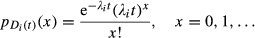
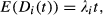
Having established the manufacturing time distributions that we consider in this study, that is, the PH(α,S,k) and Gamma(μ,k) distributions, we next turn our attention to item demand. The items being manufactured face exogenous, discrete, independent, and identically distributed (IID) demands, whose distribution is item‐specific. Back orders are allowed and incur a cost penalty per unit back ordered per unit time, while produced and unsold items incur a per unit inventory holding cost per unit time. Furthermore, both types of costs are stationary with respect to time. Given that demands are discrete and IID, we model them as being generated by a Poisson process. Letting demand for item i by time t be denoted by


To complete the description of our manufacturing setting requires that we posit production‐inventory and production‐scheduling policies, that is, when to release production orders, how many units of each item to produce and stock, and in what sequence to process the production orders. Unfortunately, for the system of interest the optimal forms of these policies are unknown. However a base‐stock policy has been shown to be optimal for a similar system under periodic review (see DeCroix and Arreola‐Risa 1998) and under continuous review (Zipkin 2000). Hence we adopt a base‐stock policy as our production‐inventory policy for the manufacturing setting under study. At the same time, given its widespread usage, we select first‐in first‐out (FIFO) as the production‐scheduling policy.
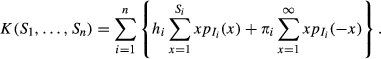
We now formally define the notation of our model. Let:
K = long‐run average inventory holding and back ordering cost per unit time
n = number of items.


The long‐run average inventory holding and back ordering cost per unit time is then:
If we define


Multi‐Item Production Systems
In this section we investigate production systems with multiple items. We divide our study of such systems into two cases: homogeneous items and heterogeneous items. In the homogeneous items case the cost and demand parameters of items are identical, but the items are physically different, such as in flavor or color. In the heterogeneous items case not only are the items physically different, but it is also true that the cost and demand parameters are no longer the same.
In one of the consulting projects alluded to in section 1, items were heterogeneous, while in the other consulting project, which involved multiple plants, in one of the plants items were homogeneous, in several other plants the items were heterogeneous, and in one plant a single item was going to be produced. We consider production systems with heterogeneous items in subsection 3.1, while in subsection 3.2, we turn our attention to production systems with homogeneous items. In section 4, we present results for single‐item production systems.
Heterogeneous Items
In this subsection we investigate manufacturing systems that produce multiple heterogeneous items. Such systems are widespread and can be found in industries as varied as food, clothing, and electronics.
Before presenting our first major results on production systems with multiple heterogeneous items, we need to establish some additional notation. Let λ denote the average total demand rate for the n items produced, where


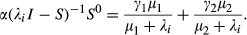
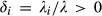
For a production system with multiple heterogenous items, when M has a PH(α,S,k) distribution or a Gamma(μ,k) distribution, stockless operation is optimal, if and only if for each item i
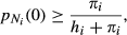


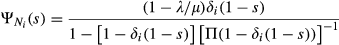
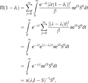
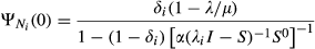
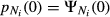
Let In Online Appendix S1 we derive that when M has a PH(α,S,k) distribution, When M is modeled as having a Gamma(μ,k) distribution, in Online Appendix S2 we derive that Because Note that the condition in inequality is equivalent to the newsvendor argument: if


We next discuss several research findings and managerial implications that follow from the result in Theorem , and then present two corollaries of the theorem, respectively called Corollaries 1 and 2.
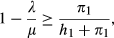
First observe that the right‐hand side (RHS) of the inequality in is a version of the well known critical fractile of the newsvendor model. This fractile plays an important role in many un‐capacitated, one‐period inventory management problems. It is intuitively pleasing to find the same fractile playing a role in our capacitated, multi‐period, production‐inventory system setting. Similar findings have been reported in some of the research already cited (de Vericourt et al. 2000, Veatch and de Vericourt 2003, Veatch and Wein 1996, Zheng and Zipkin 1990).
Further examination of Theorem allows us to deduce an intriguing property of production systems with heterogeneous items: because


For a production system with multiple heterogenous items, when M has a PH(α,S,k) distribution, stockless operation is optimal, if and only if for each item i
From Equation we have that Replacing


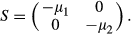
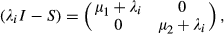
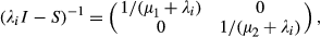
To illustrate the application of Corollary , say for example that after some experimentation the production system designer decides to capture the behavior of M as the mixture of two exponential distributions with parameters


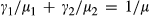

Hence

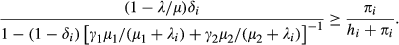
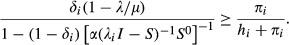
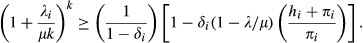
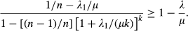
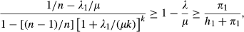
For a production system with multiple heterogenous items, when M has a Gamma(μ,k) distribution, stockless operation is optimal, if and only if for each item i
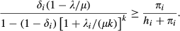
Combining equations Equations and yields

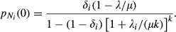
Inspection of the expression in shows the condition for the optimality of stockless production is clearly dependent on both design variables: manufacturing speed (μ) and manufacturing consistency (k). In addition, the managerial implication of Corollary confirms our intuition: given the terms (1 − λ/μ) > 0 and
In the remainder of this section we will establish two propositions that should be of value to production system designers. Let
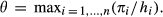
Consider a production system with multiple heterogenous items, where M has a Gamma(μ,k) distribution. Let If the production system is designed to operate at a manufacturing speed μ greater than If the production system is designed to operate at a manufacturing speed μ lower than


We know from Theorem that it is optimal for the production system to be stockless, if and only if for each item i
From basic principles we have that for any item i
Thus if for each item i
To prove part (ii), we know from Corollary that for the production system under study, it is not optimal to be stockless if and only if for each item i
But since

Proposition tells us that when the manufacturing speed is “fast enough,” that is, μ exceeds the threshold

Of special interest is the fact that


Using Proposition we obtain that

Although for the above example Proposition provides guidance when the manufacturing speed is


If a production system with multiple heterogeneous items is designed to operate at a manufacturing speed μ in the range


We know from Corollary that it is optimal for the production system to be stockless, if and only if for each item i
We also know from Equation that the LHS of inequality is always positive. In turn,

Returning to our example of Company B, Proposition tells us that for a production system with for instance a manufacturing speed μ = 140, where


Production system designers can utilize Propositions and to generate “design tables” that list

Design Table for Company B

In order to determine the production system design to adopt, system designers would factor in the capital and operating expenditures associated with each option in the design table. This is precisely what system designers did in our consulting work with minor variations depending on project idiosyncracies.
In this subsection we consider manufacturing systems that produce multiple homogeneous items. An example of such a system can be found in a firm that engages in the production of both pink and blue baby shoes. In such a setting it is not unreasonable to expect that the cost and demand parameters for both colors would be almost identical.
To facilitate a comparison between heterogeneous and homogeneous multi‐item production systems, in this subsection the subindex i = 1 will be used to denote each and every one of the n homogeneous items. In the following corollary, we establish the role that the variables manufacturing speed and manufacturing consistency play in the design of multi‐item production systems with homogeneous items.
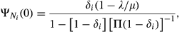
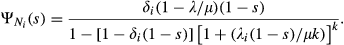
For a production system with multiple homogeneous items, when M has a Gamma(μ,k) distribution, stockless operation is optimal, if and only if Moreover,
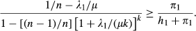
where 
Observe that when items are homogeneous, 

Two managerial implications arise from Corollary that seemingly run counter to the principle of risk pooling. We have that as demands for items are combined or pooled, the likelihood of stockless production being optimal is reduced. In addition, whether or not demand pooling actually affects the optimality of stockless production depends on several factors. These two managerial implications are illustrated next via an example and then formalized in a proposition.
Consider Company C, which is designing a production system with homogeneous items that come in two basic colors (blue and red), and in turn each color comes in four modalities (1, 2, 3, and 4). Thus we have a total of eight homogenous items, where for instance, B1 denotes blue in modality 1 and R4 denotes red in modality 4. The parameters of these eight homogenous items are as follows: 


If Company C then decides, for each color, to pool the demands of modalities 1 and 2 into modality 5, and pool the demands of modalities 3 and 4 into modality 6, we have the following parameters for the resulting four homogeneous items: 


Finally, if Company C decides for each color to pool the demands of modalities 5 and 6 into a single modality 7, the resulting parameter values of the two homogeneous items are 


In short, sometimes pooling will preserve the optimality of stockless production and sometimes it will not. Put another way, we now know that while pooling will always be desirable for companies where it is optimal to have inventories, the same cannot be said for firms that want to achieve stockless production. This reality was discovered in the consulting project with the oil and gas company mentioned in section 1 of this paper.
The dynamic between pooling and stockless production, illustrated above, is captured in the following proposition.
Let 

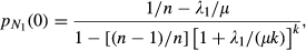
Consider a production system with multiple homogeneous items, where M has a Gamma(μ,k) distribution. Define Risk pooling always works against the optimality of stockless operation. If If Otherwise, risk pooling will affect the optimality of stockless production if and only if 


We will first prove the result in (i). In Online Appendix S3 we demonstrate that the LHS of inequality is an increasing function of n for n ≥ 1. At the same time, risk pooling induces a reduction of n, which decreases the LHS of inequality . Given that risk pooling decreases the LHS of inequality but leaves unchanged the RHS of inequality , means that risk pooling always works against the optimality of stockless operation. Combining the definition of In turn, substituting n = 1 in the LHS of inequality yields 1 − λ/μ. Therefore, because the LHS of inequality is an increasing function of n for n ≥ 1, we have that Hence if If 


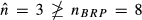
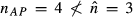
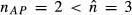
The predictive power of Proposition can be seen by revisiting the Company C example. From the inequality in a we determine 


The intuition behind the impact of risk pooling on the optimality of stockless production, that emanates from Corollary and is captured in Proposition , is as follows: We know from Corollary that the optimality of stockless operation depends on the relationship between Inspection of Recall from Online Appendix S1 that Note that for homogeneous items, as demand is pooled, n decreases and thus Given that as demand is pooled, Because risk pooling reduces The result in (ii) says that if it is not optimal for the initial homogeneous items to be stockless, then risk pooling will not help because it always works against the optimality of stockless operation. The result in (iii) says that if it is optimal to have a stockless operation in the extreme case where the initial homogeneous items would be pooled into a single item, then any lesser amount of risk pooling would not affect the optimality of stockless operation. The result in (iv) says that if it is optimal for the initial homogeneous items to be stockless, and it is not optimal to be stockless in the extreme case where the initial homogeneous items would be pooled into a single item, then there exists a “threshold” amount


Having investigated production systems with multiple items, we now turn our attention to production systems with a single item. Our motive is two‐fold. First, as we mentioned earlier, in the consulting project with multiple plants, one of the stockless production systems being designed at one plant involved only a single item. Second, as we shall demonstrate, stockless single‐item production systems permit results that are parsimonious, and at the same time, more general than the results in Theorem . Since there is only one item, the subscript i will be omitted.
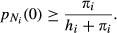
Consider a production system with a single item. For any distribution of unit manufacturing time M and any distribution of demand D, stockless operation is optimal, if and only if
Using similar arguments to those in the proof of Theorem , but where now M and D are generally distributed, we know that it is optimal for the single item to be stockless, if and only if We also know that when M and D are generally distributed, the processing of orders at the manufacturing facility corresponds to a G/G/1 queueing system. Recalling that for a G/G/1 queueing system 
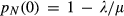
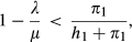
Several research findings and practical implications follow from the result in Corollary . First, while for multiple‐item systems the expressions in , , and eluded an interpretation, an understanding of the conditions for a stockless design to be optimal in a production system with one item is within reach: The manufacturing rate must exceed the demand rate by an amount equal to λπ/h. In turn, this amount is directly related to the demand rate (λ) and to the ratio of the demand back ordering cost rate to the inventory holding cost rate (π/h). The values π and h are inconsequential; it is the ratio π/h that matters.
Our second research finding concerns the already noted trade‐off faced by production system designers: manufacturing speed vs. manufacturing consistency. Corollary tells us that the optimality of stockless operation for a production system with a single item is independent of k and thus of manufacturing consistency. The practical implication of this research finding is surprising: manufacturing speed matters and manufacturing consistency does not. However, it is more surprising that this finding is entirely in agreement with our findings in the multi‐item case, where both manufacturing speed and manufacturing consistency do play a role. Recall that in a multi‐item production system the value of k is relevant when 


Our third research finding, one already mentioned in our statement of Corollary , is that the optimality of stockless operation in a single‐item production system is independent of the distributions of demand and unit manufacturing time. This finding in combination with the second one above yields the following general principle: In cases where a designer does not know the distribution of demand and unit manufacturing time, the designer only needs to focus on the variable manufacturing speed when working on the design of a stockless production system with one item.
In this section we detail how the research results contained in this study were applied to an oil and gas company project. Unconventional oil is petroleum extracted using techniques other than the conventional (oil well) method. Oil industries and governments across the globe are investing in unconventional oil sources due to the increasing scarcity of conventional oil reserves. The Research & Development Division of Company Alpha has developed over several years two technologies for unconventional oil. We will refer to these technologies as technology Y and technology Z. The resulting product from each technology is a sophisticated, heavy, bulky, and expensive apparatus that would be deployed in the ground, by a so‐called deployment crew.
For brevity, the resulting products of each technology will simply be called item Y and item Z, respectively. With the exception of a vital feature involving intellectual property which cannot be described in this article, items Y and Z are identical. Even though it is an oversimplification, the reader may think of two almost identical automobiles, where in one of them the steering wheel is on the right and in the other one the steering wheel is on the left.
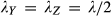
Company Alpha is interested in taking technologies Y and Z from Research & Development to large‐scale production. For this purpose, the firm launched a multi‐year project to design a supply chain that would make large‐scale production economically feasible. One of the strategic decisions that Company Alpha faced in the supply‐chain project was whether to take one of the two technologies to large‐scale production, from now called Strategy 1, or take both technologies to large‐scale production, from now on called Strategy 2. Under Strategy 2, the production and deployment of items Y and Z would be divided equally due to their symmetry.
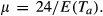
Company Alpha started the supply‐chain design project by focusing on the last two supply chain stages: Final assembly and deployment. The tactical decisions for these two stages were the average deployment rate and the average final assembly rate that would make stockless operation optimal. Several final assembly plant designs were being proposed, but in all of them items would be assembled one at a time. Additionally, the average deployment rate would be the result of the average deployment time per unit in combination with the number of deployment crews. For example, if the average deployment time per unit is 12 hours and there are five deployment crews, then the resulting average deployment rate would be 10 units per day.
Let 


Let 


Further analysis required the specification of the probability distributions of the deployment rate D and the final assembly time per unit 

Due to these circumstances, we first decided to model the deployment of one unit by one deployment crew as a point process. Point processes are one of the most general types of stochastic processes (Cox and Isham 1980). Subsequently, because D is equivalent to the superposition of the deployment processes of the N deployment crews, and N was estimated to be a very large number, based on the behavior of the superposition of a large number of points processes (Çinlar 1968), we proposed to model D as a Poisson process with parameter λ. Regarding 

Due to their symmetry, the unit production cost of items Y and Z, denoted by c, was the same. The value of c depended on the final design of items Y and Z and the market prices of several raw materials and metals including carbon steel, stainless steel, and copper. Letting h be the per unit inventory holding cost per period and r the per inventory holding cost per period expressed as a percentage, then h = rc. In addition, the cost of having a deployment crew waiting for an item to deploy was π per period, where the value of π was calculated from various oil prices and other economic variables.
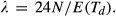
Uncertainty about parameter values such as For Strategy 1, Corollary was used to determine the minimum value of μ that the final assembly process should be designed to have for stockless operation to be optimal. We also knew from Corollary that any variability in the assembly times resulting from a design of the final assembly process could be safely ignored. For Strategy 2, based on Proposition we knew that the final assembly process should be designed to have a value of Proposition was used to explain why a final assembly process design with its associated μ and k values that made a stockless operation optimal under Strategy 2, may or may not be optimal under Strategy 1.


Conclusion
We studied a multi‐item manufacturing setting with demand‐ and production‐related uncertainty, where the problem is to design a production system so that stockless operation will be optimal. We focused on gaining an understanding of the effect of two variables that are commonly encountered in the design of production systems: manufacturing speed and manufacturing consistency. We derived conditions on these variables that establish when stockless operation is optimal. These conditions can be used by production system designers along with information on equipment costs, information costs, and execution costs to arrive at an optimal production system design. We illustrated the application of some of our results in a real‐world project at an oil and gas company.
Our work also yielded several important research findings and managerial implications. First, for stockless production systems with multiple items, both design variables play a role, while for single‐item stockless production systems manufacturing speed matters but manufacturing consistency does not. A second research finding is that even though the optimal design of a multi‐item stockless production system depends on the distributional form of demand and unit manufacturing times, this is not the case for a single‐item stockless production system. A third finding pertains to stockless production systems with heterogeneous items: The optimality conditions for the design variables are only a function of the total demand; in other words, the optimality of one item being or not being stockless is independent of the number of other items in the production system. On the other hand with homogeneous items, a fourth research finding is that the likelihood of stockless production being optimal declines as the demands of different products are pooled, that is, there is essentially a reverse risk pooling effect. Demand pooling could also invalidate the optimality of a stockless production system.
Several avenues may be pursued to extend the preliminary results of the study. Although modeling demand as a Poisson process served our exploratory needs well, it would be of theoretical and practical interest to obtain results for multi‐item production systems when the Poisson process is generalized to a renewal process. Consideration of more complex production systems with multiple manufacturing stages should be worth investigating too. Additional demand back ordering cost structures may be of interest as well.
Footnotes
Acknowledgments
We want to thank Professor William E. Stein for his constructive suggestions to improve this paper. We are also grateful to the reviewers and the senior editor. This paper is much better because of them.