The Backroom Effect in Retail Operations

Abstract

Traditional inventory models fail to take into account the dynamics between the retail sales floor and the backroom, commonly used by retailers for extra storage. When a replenishment order for a given item arrives at a retail store, it may not fit on the allocated shelf space, making backroom storage necessary. In this article, we introduce the backroom effect (BRE) as a consequence of misalignment of case pack size, shelf space, and reorder point. This misalignment results from the fragmented nature of inventory policy decision making in the retail industry and affects basic trade‐offs in inventory models. We specify conditions under which the BRE exists, quantify the expected amount of backroom inventory, derive an optimal short‐term inventory policy, and assess the impact of the BRE on the optimal inventory policy and total costs. Our results indicate that ignoring the BRE leads to artificially high reorder points and higher total costs. The paper concludes with a discussion of theoretical and managerial implications.

Keywords

backroom effect case pack quantity reorder point inventory management retail operations

1. Introduction

Procter & Gamble refers to the moment after a shopper arrives at the retail shelf as the “first moment of truth” (Nelson and Ellison 2005), noting the profound effect that this experience can have on branding, sales, and the supply chain. If the product is out of stock, the shopper might decide to purchase a substitute product, visit a competitor's store, delay purchase, or forgo the purchase altogether (e.g., Campo et al. 2000). Traditional inventory models do not take into account various circumstances that are unique to a retail setting. The purpose of this study is to highlight one such issue, namely, the backroom effect which arises as a consequence of poor alignment among case pack size, shelf space, and the reorder point.

In most retail stores, inventory is held in two locations, that is, on retail shelves and in the backroom. First, shelf space is both valuable and limited. Thus, storing some inventory in the backroom frees up shelf space for displaying a wider product assortment to potential customers and potentially increasing sales. Second, a replenishment order may not fit on the allocated shelf space upon arrival, as there may not be enough empty space on the shelf. Hence, the backroom provides a place to store excess inventory, which we will refer to as “overflow” inventory, instead of having to return the products that do not fit on the shelf. But storing inventory in two locations (shelf and backroom) has disadvantages. First, it leads to increased costs. Between replenishments, store management must monitor shelf and backroom inventories, and replenish the shelves from the backroom as shelf space becomes available when consumers make purchases. Second, storing inventory in the backroom increases operational complexity. Items can be misplaced or completely forgotten in the backroom, leading to inventory record inaccuracies (IRI) and lost sales (DeHoratius and Raman 2008, Raman et al. 2001). Thus, storing inventory in the backroom substantially changes the nature of the optimization problem faced by retailers, which we call the backroom effect (BRE).

It can be argued that the amount of inventory stored in the backroom is a function of the order quantity, the allocated shelf space, and the reorder point. Ideally, these decision variables would be optimized jointly to arrive at an inventory policy that is globally optimal. However, in practice, a retailer's inventory policy is defined piecewise and independently by distinct parties. The case pack size is generally decided unilaterally by the supplier and often becomes the effective store‐level order quantity. The shelf space allocation decisions are typically made only periodically (e.g., semi‐annually) and are largely controlled by a retailer's merchandising department. Thus, in the short run, retail operations can only change the reorder point to affect the dynamics between the retail sales floor and backroom and more generally to minimize costs.

This study contributes to the inventory management literature by modeling the BRE in a typical retail setting. First, we specify conditions under which BRE may be observed. Second, we derive an expression for the expected amount of overflow inventory which reveals complex interactions among case pack size (order quantity), reorder point, shelf capacity, and lead time demand. Third, we explore the impact of the BRE on a traditional (baseline) total cost model that includes purchasing, ordering, backorder, and inventory holding costs. Finally, we use numerical simulation to assess whether ignoring the BRE can have significant negative effects on operational costs.

The remainder of this article is organized as follows: In section 2, we briefly review relevant literature. In section 3, we quantify the BRE and assess its impact on a traditional inventory model. We also present the results of our numerical simulation. Section 4 presents major results, insights, theoretical and practical implications, limitations, and further research ideas.

2. Literature Review

Most items shipped to a retail store are replenished in case packs. For a retail store that replenishes its inventory using an (r, Q) replenishment policy, the case pack size becomes the store's effective order quantity. Alternatively, a retailer may use an (r, nQ) policy to replenish, such that the orders are integer multiples of the case pack (Chen 2000, Donselaar et al. 2010, Hill and Johansen 2006, Veinott 1965). Regardless of which replenishment policy it uses, case pack size significantly affects store operations (Ferguson and Ketzenberg 2006, Ketzenberg and Ferguson 2008) through two primary influences. First, larger case packs reduce the frequency with which the store must be replenished, which improves the stock‐keeping unit's (SKU's) fill rate. Second, larger case packs increase the probability that not all units fit on the shelf when the replenishment arrives at the store, thereby creating the need for backroom storage. Because replenishment from the backroom tends to be unreliable (Raman et al. 2001, Waller et al. 2008), the shelf fill rate declines when a greater percentage of units gets replenished from the backroom. That is, the unreliable replenishment occurs because inventory might be misplaced in storage (Raman et al. 2001), the store may have insufficient labor, or the business processes could be poorly designed (e.g., Gruen and Corsten 2007, McKinnon et al. 2007, Waller et al. 2008, 2010).

The issue of storage space limitation has been addressed in the inventory management literature from different perspectives. Some studies have addressed the effect of storage space limitation, along with other constraints, under deterministic demand (e.g., Haksever and Moussourakis 2005, Hariga and Jackson 1995). Other studies treat demand as stochastic and propose various optimal inventory policies. For example, Beyer et al. (2001) study a multi‐item inventory model with stochastic demands and a restriction on the total storage space. Minner and Silver (2005) consider a similar problem where they assume zero lead times and do not allow backordering. Hariga (2010) models a single item continuous review system and limited warehousing space where excess inventory has to be returned to the supplier. Our model differs from those in previous studies in that (i) inventory is stored in two locations, that is, on the shelf with limited capacity and in the backroom with unlimited capacity and (ii) the only decision variable is the reorder point.

3. Modeling Framework

3.1. Modeling the Backroom Effect

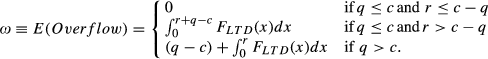
Overflow inventory (the amount of inventory that does not fit on the shelf when a replenishment order arrives at the retail store) lies at the heart of the BRE. Overflow inventory is stored in the backroom and subsequently used to replenish the shelf as shelf inventory declines due to consumer purchases. To model the overflow, consider a retail store which uses a continuous review system to replenish a single SKU with a lead time demand distribution F _LTD(x), an allocated shelf capacity of c units, a reorder point of r units, and a case pack size of q units, which becomes the retailer's effective order quantity. When the case pack size is less than or equal to the difference between the shelf capacity and the reorder point (q ≤ c−r), the probability of overflow is zero, as the shelf will always have enough empty space to accommodate a replenishment order. By extension, the expected amount of overflow is also zero. When the case pack size is strictly greater than the shelf capacity (q > c), the probability of overflow becomes 1 since a case pack will never fit the allocated shelf space even if there is no inventory on the shelf. In this case, the amount of overflow depends on lead time demand. If lead time demand, x, is equal to or greater than the reorder point, there will be no shelf inventory when the replenishment arrives, and the overflow amount will be (q−c). However, if lead time demand is less than the reorder point, there will be some inventory on the shelf (r−x), and the overflow amount will equal ([q−c] + [r−x]). Thus, the expected amount of overflow per order cycle is

\begin{matrix} E (Overflow) & = \int_{0}^{r} (r + q - c - x) f_{LTD} (x) dx + \int_{r}^{\infty} (q - c) f_{LTD} (x) dx = (r + q - c) \int_{0}^{r} f_{LTD} (x) dx \\ - \int_{0}^{r} x f_{LTD} (x) dx + (q - c) \int_{r}^{\infty} f_{LTD} (x) dx = (r + q - c) F_{LTD} (r) \\ - \int_{0}^{r} x f_{LTD} (x) dx + (q - c) (1 - F_{LTD} (r)) = (q - c) + r F_{LTD} (r) - \int_{0}^{r} x f_{LTD} (x) dx = (q - c) + r F_{LTD} (r) \\ - (r F_{LTD} (r) - \int_{0}^{r} F_{LTD} (x) dx) = (q - c) + \int_{0}^{r} F_{LTD} (x) dx . \end{matrix}

When the case pack size is less than or equal to c, but strictly greater than c−r, there may or may not be overflow depending on lead time demand. If the lead time demand, x, is less than (r + q−c), the amount of overflow is (r + q−c−x). Otherwise, it is 0. Consequently, the expected amount of overflow per order cycle can be written as

\begin{matrix} E (Overflow) & = \int_{0}^{r + q - c} (r + q - c - x) f_{LTD} (x) dx = (r + q - c) \int_{0}^{r + q - c} f_{LTD} (x) dx - \int_{0}^{r + q - c} x f_{LTD} (x) dx \\ = (r + q - c) F_{LTD} (r + q - c) - \int_{0}^{r + q - c} x f_{LTD} (x) dx = (r + q - c) F_{LTD} (r + q - c) \\ - ((r + q - c) F_{LTD} (r + q - c) \int_{0}^{r + q - c} F_{LTD} (x) dx) = \int_{0}^{r + q - c} F_{LTD} (x) dx . \end{matrix}

As can be seen, overflow inventory and BRE are driven by a complex interaction among shelf capacity, case pack size (order quantity), and reorder point. Consolidating the above results, the expected amount of overflow per order cycle is expressed as

ω \equiv E (Overflow) = {\begin{matrix} 0 & if q \leq c and r \leq c - q \\ \int_{0}^{r + q - c} F_{LTD} (x) dx & if q \leq c and r > c - q \\ (q - c) + \int_{0}^{r} F_{LTD} (x) dx & if q > c . \end{matrix}

3.2. The Optimal Reorder Point

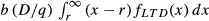
Overflow inventory, stored in the backroom, leads to additional operational costs that can be incorporated into a traditional (baseline) inventory model. The baseline model assumes backordering is allowed, and the expected total cost per year can be written as

T C_{0} (r | q, c) = v D + a \frac{D}{q} + b \frac{D}{q} \int_{r}^{\infty} (x - r) f_{LTD} (x) dx + h (r + \frac{q}{2} - E (LTD)) .

The first term, v D, represents the annual purchasing cost as a product of unit item cost v and expected annual demand D. The second term, a (D/q), refers to the annual ordering cost, where a is unit ordering cost and (D/q) is the number of orders per year. The third term,

b (D / q) \int_{r}^{\infty} (x - r) f_{LTD} (x) dx

, denotes the backorder cost, where b is the unit cost for each backordered item. The expected annual inventory holding cost is approximated as

h (r + q / 2 - E (LTD))

(for derivation, see Appendix A).

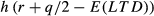
We augment the baseline expected total cost with the expected cost of BRE,

k (D / q) ω

, where k is the unit BRE cost for each item that does not fit on the shelf at the time of replenishment. Thus, the augmented expected total cost per year can now be written as

T C_{1} (r | q, c) = v D + a \frac{D}{q} + b \frac{D}{q} \int_{r}^{\infty} (x - r) f_{LTD} (x) dx + h (r + \frac{q}{2} - E (LTD)) + k \frac{D}{q} ω .

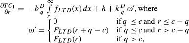
To find the optimal reorder point, we take the first and second derivatives of the expected total cost per year with respect to reorder point:

\begin{matrix} \frac{\partial T C_{1}}{\partial r} = & - b \frac{D}{q} \int_{r}^{\infty} f_{LTD} (x) dx + h + k \frac{D}{q} ω^{'}, where \\ ω^{'} = {\begin{matrix} 0 & if q \leq c and r \leq c - q \\ F_{LTD} (r + q - c) & if q \leq c and r > c - q \\ F_{LTD} (r) & if q > c, \end{matrix} \end{matrix}

\begin{matrix} \frac{\partial^{2} T C_{1}}{\partial r^{2}} = & b \frac{D}{q} f_{LTD} (r) + k \frac{D}{q} ω^{″}, where \\ ω^{″} = {\begin{matrix} 0 & if q \leq c and r \leq c - q \\ f_{LTD} (r + q - c) & if q \leq c and r > c - q \\ f_{LTD} (r) & if q > c . \end{matrix} \end{matrix}

Note that as ∂² TC ₁/∂r ² ≥ 0 for all r > 0 the expected total cost per year is convex. To derive the optimal reorder point, we consider two different cases: (i) q ≤ c and (ii) q > c.

Case
q ≤ c

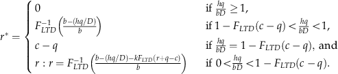
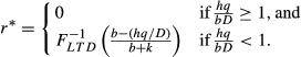
When q ≤ c, it can be shown that the optimal reorder point is
$\frac{hq}{bD}$

(For derivation, see Appendix B.)

Equation indicates that the “I/B” ratio, that is, hq/bD, plays an important role in determining the optimal reorder point. In the I/B ratio, h signifies the annualized inventory carrying cost percentage, whereas b refers to the cost of backordering a single item during a given order cycle. Hence, b is annualized when multiplied by D/q, the number of order cycles in a year. As such, the I/B ratio can be interpreted at the relative magnitude of unit inventory carrying cost compared to the unit backorder cost adjusted by order frequency. In other words, the I/B ratio represents the trade‐off between inventory carrying costs and backorder costs.

As Equation shows, the optimal solution can take on different forms depending on the particular value of the I/B ratio. Specifically, when the I/B ratio is greater than or equal to 1, the optimal solution is found at r* = 0 as the slope of the expected total cost becomes non‐negative at r = 0. 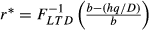When the I/B ratio is less than 1, the optimal solution depends on the location of the I/B ratio relative to a threshold determined by the lead time demand, that is, 1–F _LTD(c–q) = P(LTD > c–q). Above this threshold, the optimal reorder point becomes
$r^{} = F_{LTD}^{- 1} (\frac{b - (hq / D)}{b})$
, which is less than c–q and hence BRE is not observed (Figure a). In this region, the baseline and augmented expected total cost functions (TC ₀ and TC ₁) overlap. As a result, this can be considered the baseline solution. Below this threshold, however, the optimal reorder point exceeds c−q; hence BRE exists and the unit BRE cost k enters the solution (Equation ). Note that TC ₀ and TC ₁ diverge when r > c–q due to the existence of the BRE (Figure b). It can be shown that the reorder point
$r_{0}^{}$
that minimizes the baseline expected total cost function TC ₀ (which ignores BRE) is greater than the reorder point
$r_{1}^{}$
that minimizes the augmented expected total cost function TC ₁.

Figure 1
Expected Total Cost Per Year (q ≤ c)

Case
q > c

When q > c, BRE is always observed and the optimal reorder point can be expressed as
$r^{} = {\begin{matrix} 0 & if \frac{hq}{bD} \geq 1, and \\ F_{LTD}^{- 1} (\frac{b - (hq / D)}{b + k}) & if \frac{hq}{bD} < 1 . \end{matrix}$

(For derivation, see Appendix B.)

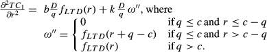
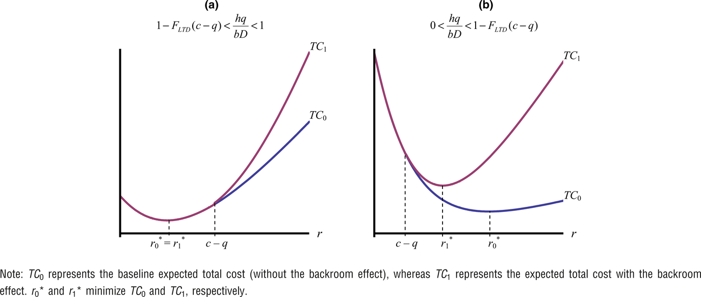
As in the previous case, the I/B ratio drives the behavior of the optimal solution. However, the lead time demand loses its role in setting a threshold as BRE exists for all values of r. When the I/B ratio is greater than or equal to 1, the optimal reorder point becomes 0. But when the I/B is less than 1, there is only a single solution, which is very similar to the baseline solution except that the unit BRE cost, k, enters the solution due to the presence of the BRE (Figure ). It can be shown that the reorder point
$r_{0}^{}$
that minimizes the baseline expected total cost function TC ₀ (which ignores BRE) is greater than the reorder point
$r_{1}^{*}$
that minimizes the augmented expected total cost function TC ₁.

Figure 2
Expected Total Cost Per Year (q > c)

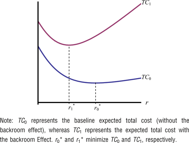
Taken together, the results in Equations and highlight a number of important insights about the dynamics between the backroom and retail sales floor. First, the BRE exists within certain parameter ranges. These ranges reflect various trade‐offs among inventory holding costs, backorder costs, and lead time demand. Second, the BRE, when it exists, changes the optimal reorder point as well as the expected total cost per year. Ignoring the BRE can lead to an artificially higher reorder point and a higher total cost. Thus, managers must take into account the BRE for improved decision making in retail operations. Next, we conduct numerical simulation to test whether the BRE affects the optimal solution and total costs to any significant degree.
3.3. Numerical Simulation

To conduct our numerical simulation, we rely on data derived from retail store audits conducted in the ready‐to‐eat (RTE) cereal category. We consider a slow selling SKU with demand rate of slightly over one unit per week, such that LTD ∼ Gamma (k = 2, θ = 2). The case pack size for this SKU is 12 (q = 12) selling units with a shelf capacity of 15 selling units (c = 15). Figure illustrates the optimal reorder point for different values of the I/B ratio, which represents the trade‐off between inventory holding and backorder costs, and k/b ratio, which represents the trade‐off between BRE costs and backorder costs. Note that the I/B ratio determines the region where BRE exists, which is between 0 and 1−F _LTD(15−12) ≅ 0.56 in this particular case. Above this threshold, BRE does not exist and consequently there is a single curve that characterizes the optimal reorder point in this region. When BRE exists, the optimal reorder point deviates from the baseline depending on the ratio between BRE cost and backorder cost. This difference grows as k increases relative to b. This difference is also amplified with increasing demand. To illustrate, suppose that inventory holding cost is the same as the backorder cost (h/b = 1), and the case pack size q = 12. For an SKU with expected annual demand D = 60 units/year, the I/B ratio

\frac{hq}{bD} = 0.2

, and the deviation from the optimal reorder point is already discernable for different values of k/b. As the annual demand doubles from 60 to 120 units/year, the I/B ratio decreases by half, but the deviation from the optimal reorder point becomes more substantial. Thus, for faster selling SKUs, it is even more important to consider the BRE when determining the reorder point.

Figure 3

Optimal Reorder Point

Figure shows the percentage increase in expected total cost per year when BRE is ignored in calculating the optimal reorder point. More precisely,

Δ = \frac{T C_{1} (r_{0}^{*}) - T C_{1} (r_{1}^{*})}{T C_{1} (r_{1}^{*})} \cdot 100 %

, where r ₀* and r ₁* minimize TC ₀ and TC ₁, respectively. When the I/B ratio is between 1−F _LTD(15−12) and 1, the BRE does not exist; hence, r ₀* equals r ₁* and the percentage difference diminishes to zero. Outside this range, an additional cost is incurred for ignoring the BRE and using r ₀* instead of r ₁*. The cost of using the suboptimal reorder point rises as the unit BRE cost k increases. Furthermore, demand rate amplifies the negative effect of using a suboptimal reorder point. Figure shows that, for the selected parameter values, the cost of ignoring BRE can grow to substantial levels.

Figure 4

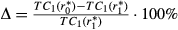
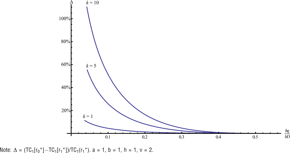
Percentage Difference in Total Cost when the Backroom Effect is Ignored

4. Concluding Discussion

Over the last decade, academic research has begun to provide evidence that retail store execution is one of the most substantial challenges to the proper functioning of a retail supply chain (DeHoratius and Raman 2008, Donselaar et al. 2006, Raman et al. 2001, Ton and Huckman 2008, Ton and Raman 2010). Cumulatively, these findings suggest that even careful planning may result in undesirable outcomes due to poor store execution (Fisher et al. 2009). Adding to the complexity of store execution problems is use of the retail backroom to replenish the sales floor, which results in the BRE.

In this study, we present a modeling framework to explore the BRE on inventory decision making and retail operations. We derive closed‐form expressions for the probability of overflow, expected amount of overflow, and costs associated with overflow. When the BRE considerations are included in a traditional inventory model, they significantly alter the nature of the problem and the optimal inventory policy. A new trade‐off between BRE cost and backorder cost, k/b, enters the optimal solution in addition to the trade‐off between inventory holding cost and backorder cost. Numerical simulation results show that ignoring the BRE can lead to substantially worse inventory decisions for a retailer.

Although prior studies have documented the significant effects of BRE on a retailer's operational performance (e.g., Waller et al. 2010), no research has provided a way to quantify the BRE. Our analytical work formalizes these previous empirical studies by providing a modeling framework that can quantify the magnitude of the BRE and its potential impact on retail performance. Our results indicate that the extent of the BRE is driven by an interaction among case pack size (order quantity), shelf space, reorder point, and lead time demand.

While retailers often acknowledge the BRE, they either ignore it, hoping that their suboptimal policy will not significantly deviate from the optimal policy, or try to avoid it by allocating enough shelf space to eliminate overflow inventory. The first option is not sensible, as we have shown that ignoring the BRE can lead to considerably higher operational costs. Given simplicity and versatility of our modeling framework, retailers can use commonly available software packages (e.g., Excel) to incorporate the BRE in their inventory decision‐making processes. The second option is not prudent either, as it can be wasteful to allocate additional shelf space to an SKU just to avoid overflow inventory. In fact, our results demonstrate that an optimal solution can exist in the region where BRE is observed, depending on the trade‐off between inventory holding costs and backorder costs.

Perhaps the main limitation of our study is its exclusive focus on the reorder point as its sole decision variable. In practice, a complete inventory policy includes case pack size (order quantity) and shelf capacity as decision variables, too. In fact, the BRE can be viewed as a product of misalignment among these three variables. However, such alignment and optimal decisions are difficult to achieve due to the existing fragmented approach to inventory decision making in retailing (Figure ). Although retail operations may be responsible for setting reorder points, shelf space decisions are often made by the retailer's merchandising and/or marketing organizations. Furthermore, case pack size has long constituted a site of battles between retailers and suppliers. Although case pack quantity has substantial financial and operational implications for both suppliers and retailers, it is generally determined unilaterally by the supplier on the basis of pallet dimensions, truck trailer dimensions, and packing machine capabilities (Food Marketing Institute (FMI) and the Grocery Manufacturers of America (GMA) 2000). As each party attempts to optimize the decision variable under their control, their efforts will not be completely effective in achieving full alignment (optimality) among case pack size (order quantity), shelf space, and reorder point. Hence, a promising direction for future research is to model a retailer's inventory problem from a more holistic perspective.

Figure 5

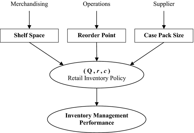
Retail Inventory Decision Making

Another limitation is our use of the simplifying assumption that the sum of the various costs associated with overflow is proportional to the amount of overflow, which may not be true in all cases. Overflow can have effects on labor requirements, shelf stockouts, and IRI costs. A more detailed description of the behavior of overflow costs, either through analytical modeling, discrete event simulation or empirical observation, can greatly enhance the applicability of our modeling framework.

Footnotes

Appendix A

Appendix B

1

Store audits were taken over a 12‐week period from several retail stores by a third‐party. During the audits, the case pack size, shelf capacity, and demand rate, along with other information, were recorded.

2

While the lead time demand is more accurately modeled with a discrete distribution, a continuous distribution is chosen in the interest of clarity of exposition.

References

Beyer

Sethi

S. P.

Sridhar

. 2001. Stochastic multi‐product inventory models with limited storage. J. Optim. Theory Appl. 111(3): 553–588.

Campo

Gijsbrechts

Nisol

. 2000. Towards understanding consumer response to stock‐outs. J. Retail. 76(2): 219–243.

Chen

2000. Optimal policies for multi‐echelon inventory problems with batch ordering. Oper. Res 48(3): 376–389.

DeHoratius

Raman

. 2008. Inventory record inaccuracy: An empirical analysis. Manage. Sci. 54(4): 627–641.

vanDonselaar

K. H.

Gaur

vanWoensel

Broekmeulen

R. A. C. M.

Fransoo

J. C.

. 2010. Ordering behavior in retail stores and implications for automated replenishment. Manage. Sci. 56(5): 766–784.

vanDonselaar

K. H.

Van Woensel

Broekmeulen

R. A. C. M.

Fransoo

J. C.

. 2006. Inventory control of perishables in supermarkets. Int. J. Prod. Econ. 104(2): 462–472.

Ferguson

Ketzenberg

. 2006. Information sharing to improve retail product freshness of perishables. Prod. Oper. Manage. 15(1): 57–73.

Fisher

M. L.

Krishnan

Netessine

. 2009. Are your staffing levels correct? Int. Commer. Rev. – ECR J. 8(2–4): 110–115.

Food Marketing Institute (FMI) and the Grocery Manufacturers of America (GMA) . 2000. Case Pack Optimization: Supply Chain Economics of Variations in Case Pack Quantities for Consumer Packaged Goods. Food Marketing Institute (FMI) and the Grocery Manufacturers of America (GMA), Washington, DC.

10.

Gruen

T. W.

Corsten

. 2007. A Comprehensive Guide to Retail Out‐of‐Stock Reduction in the Fast Moving Consumer Goods Industry. Grocery Manufacturers Association (GMA), Food Marketing Institute (FMI), National Association of Chain Drug Stores (NACDS), The Procter & Gamble Company (P&G), the University of Colorado at Colorado Springs, Washington, DC.

11.

Haksever

Moussourakis

. 2005. A model for optimizing multi‐product inventory systems with multiple constraints. Int. J. Prod. Econ. 97(1): 18–30.

12.

Hariga

M. A.

2010. A single‐item continuous review inventory problem with space restriction. Int. J. Prod. Econ. 128(1): 153–158.

13.

Hariga

Jackson

P. L.

. 1995. Time‐variant lot sizing models for the warehouse scheduling problem. IIE Trans. 27(2): 162–170.

14.

Hill

R. M.

Johansen

S. G.

. 2006. Optimal and near‐optimal policies for lost sales inventory models with at most one replenishment order outstanding. Eur. J. Oper. Res. 169(1): 111–132.

15.

Ketzenberg

Ferguson

. 2008. Managing slow‐moving perishables in the grocery industry. Prod. Oper. Manag. 17(5): 513–521.

16.

McKinnon

A. C.

Mendes

Nababteh

. 2007. In‐store logistics: An analysis of on‐shelf availability and stockout responses for three product groups. Int. J. Logistics: Res. Appl. 10(3): 251–268.

17.

Minner

Silver

E. A.

. 2005. Multi‐product batch replenishment strategies under stochastic demand and a joint capacity constraint. IIE Trans. 37(5): 469–479.

18.

Nelson

Ellison

. 2005. Shelf promotion: In a shift, marketers beef up ad spending inside stores. Wall St. J. September 21 (Eastern Edition), A.1.

19.

Raman

DeHoratius

Ton

. 2001. Execution: The missing link in retail operations. Calif. Manage. Rev. 43(3): 136–152.

20.

Ton

Huckman

R. S.

. 2008. Managing the impact of employee turnover on performance: The role of process conformance. Organ. Sci. 19(1): 56–68.

21.

Ton

Raman

. 2010. The effect of product variety and inventory levels on retail store sales: A longitudinal study. Prod. Oper. Manag. 19(5): 546–560.

22.

Veinott

A. F.

Jr . 1965. The optimal inventory policy for batch ordering. Oper. Res 13(3): 424–432.

23.

Waller

Tangari

Williams

. 2008. Case pack quantity's effect on retail market share. Int. J. Phys. Distribution Logistics Manage. 38(6): 436–451.

24.

Waller

M. A.

Williams

B. D.

Tangari

A. H.

Burton

. 2010. Marketing at the retail shelf: Exploring moderating effects of logistics on SKU market share. J. Acad. Mark. Sci. 38(1): 105–117.