Robust Stochastic Lot‐Sizing by Means of Histograms

Abstract

Traditional approaches in inventory control first estimate the demand distribution among a predefined family of distributions based on data fitting of historical demand observations, and then optimize the inventory control using the estimated distributions. These approaches often lead to fragile solutions whenever the preselected family of distributions was inadequate. In this article, we propose a minimax robust model that integrates data fitting and inventory optimization for the single‐item multi‐period periodic review stochastic lot‐sizing problem. In contrast with the standard assumption of given distributions, we assume that histograms are part of the input. The robust model generalizes the Bayesian model, and it can be interpreted as minimizing history‐dependent risk measures. We prove that the optimal inventory control policies of the robust model share the same structure as the traditional stochastic dynamic programming counterpart. In particular, we analyze the robust model based on the chi‐square goodness‐of‐fit test. If demand samples are obtained from a known distribution, the robust model converges to the stochastic model with true distribution under generous conditions. Its effectiveness is also validated by numerical experiments.

Keywords

stochastic inventory control robust optimization dynamic programming optimal policy

1. Introduction

The stochastic lot‐sizing model has been extensively studied in the inventory literature. Most of the research has focused on models with complete information about the distribution of customer demand. However, in most real‐world situations, the demand distribution is not known; only historical data are available. A common approach is to hypothesize a family of demand distributions and then to estimate the parameters specifying the distribution using the historical data. Once the probability distribution has been identified, the inventory problem is solved following this estimated distribution. This implies that the inventory policy is determined under the assumption that the fitted distribution adequately characterizes the demand to be realized in the future.

The estimated demand distribution may not be accurate, and, hence, the approach of fitting the distribution and optimizing the inventory decisions sequentially may not work as expected. As shown in Liyanage and Shanthikumar (2005) for the newsvendor model, such an approach may generate suboptimal solutions. Besides, in distribution fitting, one needs to assume a parametric family of a demand distribution in the first place, and this hypothesis may also go awry. For instance, we may fit the historical data to a lognormal distribution while it actually follows a uniform distribution.

The robust inventory models, without assuming a parametric family of distributions, provide an approach to address ambiguity in the demand distribution. A brief review of these robust models is provided in section 1.1. These models adopt a minimax approach targeting to minimize the worst case expected cost maximized over the set of distributions. Without exception, the existing literature either considers a prespecified set for demand distributions without detailed discussions about how to generate the set, for example, Notzon (1970), or derives the set of distributions based on certain statistics of the historical data such as the sample mean and variance, for example, Bertsimas and Thiele (2006) and See and Sim (2010). Compared with the classical approach with separate fitting and optimization, the robust models based on historical statistics may miss important information about the demand distribution conveyed in the historical data set, for example, the shape of the distribution, which, in the separate, two‐phase approach, is usually used to determine the parametric family of the distributions.

In this article, we merge the merits of both approaches, namely (i) to fully utilize historical data as in the classical approach and (ii) to concurrently optimize the demand distribution and the inventory decision without assuming a distribution family as in the robust models. We analyze the single‐item stochastic finite‐horizon periodic review lot‐sizing model under the assumption that the demand is subject to an unknown distribution and only historical demand observations (given by histograms) are available. As all practitioners in inventory control start with histograms and then fit an underlying demand distribution, this assumption reflects the practical value of this research.

By adopting the minimax robust optimization approach, rather than first estimating the demand distribution and then optimizing inventory decisions, we combine these two steps to minimize the worst case expected cost over a set of demand distributions, which is defined as all possible distributions satisfying the chi‐square goodness‐of‐fit test. The advantage of this approach is twofold. First, the historical data are used in the same manner as in the goodness‐of‐fit test; thus, we use all the information conveyed by the historical data that can be utilized by the goodness‐of‐fit test in distribution fitting. Second, we avoid the assumption about the parametric family of distributions, which is a must in distribution fitting. We show that the (s,S) policy remains optimal, discuss the behavior of the model as the number of samples increases, and demonstrate through a numerical study that this model outperforms (i) the classical approach where distribution estimation and inventory optimization are separate and (ii) a robust model where the set of distributions is defined by sample mean and variance.

Our two main contributions are as follows. First, we develop a robust minimax model that only requires historical data and allows correlated demand. Note that most minimax models (see, e.g., Ahmed et al. 2007, Notzon 1970) and Bayesian inventory models, for example, updating demand distributions as suggested in Iglehart (1964), in the literature can be interpreted as special cases of our framework.

Unlike the classical inventory model, which solves a single‐variate optimization problem in each period, the robust model needs to identify the ordering quantity and probability distribution represented by a vector of decision variables simultaneously. Despite this complexity, the optimal policy of the robust model still shares the same structure as the corresponding policy in the classical stochastic lot‐sizing model. In particular, the optimal policy is a state‐dependent base‐stock policy for the multi‐period inventory problem without fixed procurement costs, and a state‐dependent (s,S) policy if the fixed procurement cost is considered.

While the first contribution mainly serves as an extension to existing models, the second major contribution regards combining the statistical test in distribution fitting within a single inventory control model. We consider a special case of the general robust framework when the set of demand distributions is directly related to the chi‐square goodness‐of‐fit test. Such a distribution set can be defined by a set of second‐order cone constraints, and, hence, it is tractable to compute the (s,S) levels for each period. To the best of our knowledge, this is the first endeavor to integrate the goodness‐of‐fit statistical test with inventory optimization and to explicitly consider the shape of the distribution in a robust framework.

We also prove that the robust model based on the chi‐square test converges to the stochastic model with true demand distribution under generous conditions if samples are drawn from this distribution and they grow indefinitely. In particular, if the demand distributions are discrete, the robust model converges to the stochastic model with the true demand distribution as the number of independent samples drawn from the true distribution for each period tends to infinity. Moreover, the rate of convergence is in the order of

1 / \sqrt{k}

, where k is the number of samples. Slightly weaker results are obtained for continuous distributions. These convergence results ensure the effectiveness of the robust approach when the sample size is sufficiently large.

When the sample size is relatively small, the performance of the robust model is illustrated by means of computational experiments. We argue that the robust model based on the chi‐square test outperforms the traditional approach, which optimizes the inventory decisions by using fitted distributions, as well as the minimax robust model where the set of distributions is based on the set proposed by Delage and Ye (2010). We also provide insights on the performance of the robust model with different parameters and sample sizes.

In section 2, we describe our robust model, which incorporates historical data, and present the optimality equation in a compact form. The structure of the optimal policies is characterized in section 3. Section 4 considers a special case with robustness defined by the chi‐square goodness‐of‐fit test. We also discuss selected convergence results for the chi‐square test‐based models in the same section. The computational results are presented in section 5. Finally, additional extensions are presented in section 6. We conclude the introduction with the literature review.

1.1. Literature Review

This work is built on two streams of literature: stochastic inventory control and robust optimization. The discrete‐time stochastic inventory model has been studied since the 1950s. Scarf (1960) proposes the concept of K‐convexity and proves that the (s, S) policy is optimal in the presence of a fixed ordering cost. Since then, the research in this area has flourished. We refer the reader to Zipkin (2000) for a detailed review. The concept of K‐convexity has been generalized to attack various problems related to inventory control, for example, Chen and Simchi‐Levi (2004). Efficient algorithms, for example, Guan and Miller (2008) and Halman et al. (2009), have also been proposed to solve other more general stochastic inventory problems.

Robust optimization was pioneered by Soyster (1973), which proposes robust linear programming formulations for linear programs with coefficient uncertainty. This line of research has enjoyed popularity in recent years. Some of the important works include but are not limited to Ben‐Tal and Nemirovski (2000) and Bertsimas and Sim (2004) for robust linear programming, Ben‐Tal and Nemirovski (1998) for robust convex optimization, and Kouvelis and Yu (1997) and Bertsimas and Sim (2003) for robust discrete optimization. More relevant to this research, Iyengar (2005) and Nilim and El Ghaoui (2005) develop a robust optimization framework for dynamic programming models, extend the Bellman recursion to the robust counterpart, and investigate its computational complexity. Delage and Ye (2010) propose a data‐driven robust framework for any single‐stage optimization problem, which minimizes the maximum expectation over a set of distributions defined by the sample mean and variance. They identify sufficient conditions under which the corresponding robust problem is polynomially solvable and provide probabilistic arguments for using this model by considering a confidence region for the mean and variance as a random vector.

In this article, we apply the idea of robust optimization to inventory control models. This notion of robust inventory control is not new in the literature. The earliest work in minimax inventory control is attributed to Scarf (1958), where minimization of the maximum expected cost of the newsvendor model over all distributions with a given mean and variance is considered. Gallego and Moon (1993) present another proof of Scarf's result and consider various extensions of the model. The recent work by Natarajan et al. (2008) extends the result of Scarf (1958) by considering the set of distributions with a given mean, variance, and semivariance information. Perakis and Roels (2008) minimize the maximum regret of the newsvendor model over a convex set of distributions with certain moments and shape.

Notzon (1970) is among the earliest works that considers a minimax multiple‐period inventory model. The demand in each period is assumed to be independent, and its distribution function is ambiguous but within a specified class of distribution functions. The minimax control policy minimizes the maximum expected cost. The optimality of the (s, S) policy is proved.

Bertsimas and Thiele (2006) analyze distribution‐free inventory problems, in which demand in each period is assumed to be a random variable that takes values in a given range. The demand is assumed to be a random variable controlled by only two values: the lower and upper estimators. To capture the trade‐off between robustness and optimality, a parameter is defined to control the budgets of uncertainty at every time period. They show that for a variety of problems, the structures of the optimal policy remain the same as in the associated model with complete information about the distribution of customer demand. A related model from the base‐stock perspective is analyzed in Bienstock and Özbay (2008).

See and Sim (2010) consider a factor‐based demand model with given mean, support, and deviation measures. To obtain tractable replenishment policies, the worst case expected cost among all distributions satisfying the demand model is minimized by solving a second‐order cone optimization problem.

Ahmed et al. (2007) propose an inventory control model that minimizes a coherent risk measure instead of the overall cost function. They show that risk aversion treated in the form of coherence risk measures is equivalent to the minimax formulations, and it is proved that the optimal policies conserve the properties of the stochastic dynamic programming counterparts. They do not consider demand‐dependent evolutions.

Liyanage and Shanthikumar (2005) first provide concrete examples in a single period (newsvendor) setting, which illustrate that separating distribution estimation and inventory optimization, as is done in the classical approach, may lead to suboptimal solutions. They propose the use of operational statistics where it is assumed that the demand distribution function belongs to a specific (predetermined) family and estimate the (single) parameter of the family within an inventory optimization model.

In addition, selected recent papers also consider lost‐sale inventory problems with censored demand data, that is, the observed historical demand data excludes the lost‐sale information as the lost sales are not observable. Huh and Rusmevichientong (2009) propose nonparametric adaptive policies to solve this problem and provide a bound for the asymptotic performance, which, interestingly, is the same as the convergence rate of our model under discrete distributions.

The models by Notzon (1970) and Ahmed et al. (2007) do not take the historical data into account, and they predefine the class of distribution functions. The robust optimization approaches from Bertsimas and Thiele (2006) as well as See and Sim (2010) do not use any historical data except to determine the support, expectation, and deviation measures. On the other hand, Liyanage and Shanthikumar (2005) use historical data but predetermine the family of distributions. In fact, they consider only distributions characterized by a single unknown parameter. This is the only work besides the one proposed in this article that concurrently optimizes the ordering quantity and applies techniques in distribution fitting to determine the demand distribution. Our research combines both strategies by integrating distribution fitting with robust optimization. Specifically, we consider the set of demand distributions that satisfy a certain data fitting criterion with respect to historical data and characterize an optimal policy that minimizes the maximum expected cost.

2. Formulation of Robust Stochastic Lot‐Sizing

The classical multi‐period inventory problem considers a finite planning horizon of T periods. We assume that all shortages are backlogged. For each period t = 1,…,T, let

{\tilde{D}}_{t}

be a random variable representing demand in that period. The sequence of events is as follows.

At the beginning of each period t, the decision maker reviews the net inventory level

x_{t}

, and places an order for

q_{t}

(possibly zero) units. The procurement cost in each period t = 1,…,T − 1 includes two components: a fixed procurement cost K if

q_{t} > 0

and a unit procurement cost

c_{t}

for each unit ordered.

Assuming zero lead time, this order arrives immediately and increases the inventory level up to

y_{t}

, where

y_{t} = x_{t} + q_{t}

. After observing demand

{\tilde{D}}_{t}

, inventory holding cost is charged at a rate of

h_{t}

for any unit of excess inventory after satisfying demand

{\tilde{D}}_{t}

, and a unit backorder cost

b_{t}

is incurred for any unit of unsatisfied demand. The net inventory at the beginning of period t + 1 is reduced to

x_{t + 1} = y_{t} - {\tilde{D}}_{t}

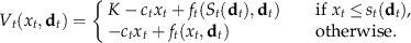
Thus, the total cost for period t given the net inventory levels before and after ordering (

x_{t}

and

y_{t}

, respectively) as well as demand

{\tilde{D}}_{t}

in that period is

C_{t} (x_{t}, y_{t}, {\tilde{D}}_{t}) = K I (y_{t} - x_{t}) + c_{t} (y_{t} - x_{t}) + h_{t} {(y_{t} - {\tilde{D}}_{t})}^{+} + b_{t} {(y_{t} - {\tilde{D}}_{t})}^{-} t = 1, \dots, T,

where

x^{+} = \max (x, 0)

x^{-} = \max (- x, 0)

I (x) = 1

if x > 0 and

I (x) = 0

otherwise.

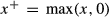
In the standard dynamic programming formulation, we consider

{\tilde{V}}_{t} (x_{t})

, t = 1,…,T, which denotes the optimal expected cost over horizon [t,T], given that the net inventory level at the beginning of period t is

x_{t}

and an optimal policy is adopted over horizon [t,T]. We assume

{\tilde{V}}_{T + 1} (x_{T + 1}) = 0

. Let θ ∈ [0,1] be the discount rate. The optimality equation reads

{\tilde{V}}_{t} (x_{t}) = \min_{y_{t} \geq x_{t}} {E [C_{t} (x_{t}, y_{t}, {\tilde{D}}_{t})] + θ E [{\tilde{V}}_{t + 1} (y_{t} - {\tilde{D}}_{t})]} t = 1, \dots, T .

Note that the distribution of

{\tilde{D}}_{t}

, t = 1,…,T is required to solve this dynamic programming formulation.

In practice, the demand distribution is not known. Rather, an inventory manager has at his or her disposal only historical data. Depending on the realized past demand in the planning horizon, the manager may choose different aggregations of historical data to forecast the demand distribution. For example,

the demand data of the last n observations are considered, which is analogous to the moving average forecast, or

the realized demand in periods 1 to t − 1 is accounted for when forecasting the demand in period t.

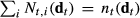
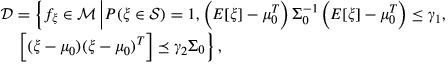
Historical observations are often aggregated to a histogram with respect to unknown distribution

{\tilde{D}}_{t}

. The bins are

[(D_{t, i}, D_{t, i + 1})]

, which denotes the ith possible range of the demand in period t (all observations within a given range are indistinguishable). Let the vector

d_{t} = [d_{1}, \dots, d_{t - 1}]

denote the realized demand in periods 1 to t − 1, where

d_{τ}

, τ = 1,…,t − 1 corresponds to the realized demand in period τ. The number of observations falling within the ith bin is a function of the realized demand

d_{t}

and is denoted by

N_{t, i} (d_{t})

. Finally, we define

n_{t} (d_{t}) = \sum_{i} N_{t, i} (d_{t})

, which corresponds to the total number of available observations under realized demand

d_{t}

. In practice, the decision maker observes only these histograms, that is, the historical samples.

We assume that

D_{t, 1} = 0

and

D_{t, M_{t} + 1} = + \infty

, where

M_{t}

corresponds to the number of bins in the histogram for time period t. Let

P_{t, i} = P ({\tilde{D}}_{t} \in [D_{t, i}, D_{t, i + 1}])

be the probability that demand in period t falls in the interval

[D_{t, i}, D_{t, i + 1}]

under the fitted distribution. Clearly,

n_{t} (d_{t}) P_{t, i}

is the expected number of observations that fall in this interval according to the fitted distribution.

The classical approach to identify the best distribution representing the observed data is to use a goodness‐of‐fit test. The objective is to fit a distribution that “closely” follows the observed data. Under this criterion, there should be a set of distributions depending on

d_{t}

, which satisfy the given goodness‐of‐fit test. We denote this set by

P_{t} (d_{t})

. Throughout this article, we assume that

P_{t} (d_{t})

is compact for any t and

d_{t}

As defined in the dynamic programming field, a decision rule

μ_{t}

at time t is a function of net inventory

x_{t}

, which decides the ordering quantity at time t given

x_{t}

, that is,

y_{t} = μ_{t} (x_{t})

. We formally state our problem in the context of a two‐player game, which is also presented in Iyengar (2005). The first player chooses the decision rule

μ_{t}

at time t and pays the cost. The second player chooses a distribution of

{\tilde{D}}_{t}

P_{t} (d_{t})

after observing the order quantity, and receives a reward equal to the cost paid by the first player. Therefore, the second player may select a different distribution for different

x_{t}

and

μ_{t}

. Let

P_{t} (x_{t}, μ_{t} (x_{t}))

denote the distribution chosen by player 2 at time t given net inventory

x_{t}

and decision rule

μ_{t}

. The set of all distributions available to player two is

Q^{μ_{t}} = {P (x_{t}, μ_{t} (x_{t})) \in P_{t} (d_{t}) over all x_{t}, d_{t}} .

Q^{μ_{t}}

we merely express that for each

x_{t}

μ_{t}

d_{t}

, we might have a different distribution. Moreover, a policy π is defined as the decision rule to be used at every period, that is,

π = (μ_{1}, \dots, μ_{T})

. A policy π also yields a set of distributions

Q^{π}

which can be used by the second player or adversary, where

Q^{π} = Q^{μ_{1}} \times Q^{μ_{2}} \times \dots \times Q^{μ_{T}} .

As the second player will maximize his or her reward, given policy π, net inventory

x_{t}

, and realized demand

d_{t}

, the cost paid by player one from period t to T is

V_{t}^{π} (x_{t}, d_{t}) = \max_{Q \in Q^{π}} E^{Q, \tilde{D}} [\sum_{τ = t}^{T} θ^{τ - t} C_{τ} (x_{τ}, μ_{τ} (x_{τ}), {\tilde{D}}_{τ}) + θ^{T + 1 - t} V_{T + 1} (x_{T + 1}, d_{T + 1})],

where

C_{τ} (x_{τ}, μ_{τ} (x_{τ}), {\tilde{D}}_{τ})

denotes the cost incurred in period τ in Equation , and

V_{T + 1} (x_{T + 1}, d_{T + 1})

is the terminal cost. Also note that Q defines the distributions

{\tilde{D}}_{τ}

, τ = t,…,T. Unless stated otherwise, we assume that

V_{T + 1} (\cdot) = 0

. We also have

x_{τ + 1} = μ_{τ} (x_{τ}) - {\tilde{D}}_{τ} and d_{τ + 1} = [d_{τ}, {\tilde{D}}_{τ}] .

Since the first player will choose a policy that minimizes the cost, the optimal cost from period t to T given net inventory

x_{t}

at time t, and the realized demand

d_{t}

from period 1 to t − 1, is

V_{t} (x_{t}, d_{t}) = \min_{π} \max_{Q \in Q^{π}} E^{Q, \tilde{D}} [\sum_{τ = t}^{T} θ^{τ - t} C_{τ} (x_{τ}, μ_{τ} (x_{τ}), {\tilde{D}}_{τ}) + θ^{T + 1 - t} V_{T + 1} (x_{T + 1}, d_{T + 1})],

for t = 1,…,T. Note that the model minimizes the maximum expected cost arising from any distribution in the set

P_{t} (d_{t})

for any t, which is known as the minimax robust approach. We next state an optimality equation, which is essential to establish the optimal control policies.

Proposition
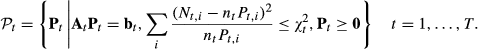
The optimality equation of the robust model is
$V_{t} (x_{t}, d_{t}) = \min_{y_{t} \geq x_{t}} \max_{P_{t} \in P_{t} (d_{t})} {\sum_{i} P_{t, i} (C_{t} (x_{t}, y_{t}, D_{t, i}) + θ V_{t + 1} (y_{t} - D_{t, i}, [d_{t}, D_{t, i}]))}$

for t = 1,…,T, where
$P_{t} (d_{t})$
is the set of distributions satisfying the goodness‐of‐fit condition at period t, and
$C_{t} (x_{t}, y_{t}, D_{t, i})$
is defined by Equation .

Proof
It follows from Theorem 2.1 in Iyengar (2005) when
$P_{t} (d_{t})$
is arbitrary. If
$P_{t} (d_{t})$
is convex, the proposition can also be proved by the von Neumann's minimax theorem (see, e.g., von Neumann 1928).

An immediate observation from Proposition is that we minimize the worst case expected cost over a set of distributions. Therefore, our robust stochastic model may not be as conservative as the classical minimax models, where the worst case is defined by the realized demand instead of distribution, for example, the minimax model discussed in section 2.4 in Notzon (1970).

Note that the Bayesian inventory models assume a prior demand distribution, and the posterior distribution at time t is obtained by updating the prior distribution using
$d_{t}$
; for example, Iglehart (1964) updates the demand distribution belonging to the exponential and range families after observing realized demand information. Our model only requires the set of distributions
$P_{t} (d_{t})$
to be a function of the realized demand
$d_{t}$
. Therefore, we can define it as a singleton updated by a Bayesian rule. In this case, the robust minimax model is reduced to a Bayesian inventory model, which indicates that the Bayesian models are special cases of our minimax model.

Proposition also gives us an interpretation of the robust model from a risk measure perspective when set
$P_{t} (d_{t})$
is convex. Ahmed et al. (2007) establish the correspondence between coherent risk measures and minimax models over convex sets of distributions. From this perspective, our minimax robust model essentially minimizes a coherent risk measure with respect to the total cost. If we consider
$P_{t} (d_{t}) \equiv P_{t}$
for any
$d_{t}$
and t, that is, the set of distributions is independent of any realized demand in previous periods, then the minimax robust model Equation minimizes a coherent risk measure in any period t and it reduces to the model considered in Ahmed et al. (2007). When the set of distributions
$P_{t} (d_{t})$
depends on demand realization
$d_{t}$
, model also minimizes a coherent risk measure in every period t. However, this model is different from that in Ahmed et al. (2007) in the sense that the risk measure in period t is updated by the realized demand in previous periods. Intuitively, if the decision maker lost a significant amount in the previous period, he or she would tend to be more risk averse in subsequent periods. Therefore, it is reasonable to adjust the risk measure based on the realized demand information
$d_{t}$
.

In addition, let constant
$p_{t}$
denote the selling price of the product in period t. We can maximize the expected total profit from periods 1 to T by subtracting term
$p_{t} \sum_{i} D_{t, i} P_{t, i}$
in the objective function of Equation . All of the results, such as the optimal policy and the convergence properties, still hold for such an objective function. In addition, if we suppose that all the distributions in set
$P_{t} (d_{t})$
could have the same expectation
${\hat{D}}_{t} (d_{t})$
, that is, constraint
$\sum_{i} D_{t, i} P_{t, i} = {\hat{D}}_{t} (d_{t})$
is included in the definition of
$P_{t} (d_{t})$
, then the models that minimize cost and that maximize profit are equivalent to each other. However, as long as the demands follow certain distributions, which are not necessarily known to the decision maker, the expected total revenue is independent of any inventory decision, that is, the order quantity in any period t. Therefore, it is sufficient to consider the cost minimization model presented in Equation .
3. Properties of Optimal Policies

In this section, we study optimal policies of the general robust stochastic model . Notzon (1970) and Ahmed et al. (2007) show the optimality of (s, S) policy when the set of distributions in the minimax model is independent of the realized demand

d_{t}

(Ahmed et al. 2007 also assume the set of distributions is convex). Here, we extend the optimality of (s, S) policy to the more general model in Equation .

We assume that the reader is familiar with standard concepts in inventory theory such as K‐convexity and (s, S) policies (see, e.g., Porteus 2002, Zipkin 2000).

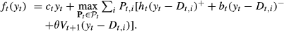
Let us define

U_{i} (y, d) = h_{t} {(y_{t} - D_{t, i})}^{+} + b_{t} {(y_{t} - D_{t, i})}^{-} + θ V_{t + 1} (y_{t} - D_{t, i}, [d_{t}, D_{t, i}]),

which corresponds to the expected cost incurred from period t to T if the inventory level after receiving the order in period t is

y_{t}

and the demand in period t is

D_{t, i}

. Consider the function

f (y, d) = \max_{P \in P (d)} \sum_{i} U_{i} (y, d) P_{i} .^{1}

Since optimality of the (s, S) policy follows directly from K‐convexity, first we are going to establish that the function f(y,d) is K‐convex in y.

Lemma
If
$U_{i} (y, d)$
is K‐convex in y for any given d, then f(y,d) is a K‐convex function in y for any given d.

Proof
Please refer to the Online Supplement.

Lemma shows that K‐convexity is preserved under maximization over a set of distributions. On the basis of this property, we show the K‐convexity of the cost‐to‐go functions.

Proposition
If
$V_{t + 1} (x_{t + 1}, d_{t + 1})$
is a K‐convex function in
$x_{t + 1}$
for any fixed
$d_{t + 1}$
, the cost‐to‐go function
$V_{t} (x_{t}, d_{t})$
is a K‐convex function in
$x_{t}$
for any fixed
$d_{t}$
, and for any t = 1,…,T.

Proof
The proposition is trivially true for t = T + 1. Suppose that the proposition holds for period t + 1, and consider period t. To simplify the notation, let us define
$f_{t} (y_{t}, d_{t}) = c_{t} y_{t} + \max_{P_{t} \in P_{t} (d_{t})} \sum_{i} P_{t, i} [h_{t} {(y_{t} - D_{t, i})}^{+} + b_{t} {(y_{t} - D_{t, i})}^{-} + θ V_{t + 1} (y_{t} - D_{t, i}, [d_{t}, D_{t, i}])] .$

Therefore, the optimality equation in is equal to
$V_{t} (x_{t}, d_{t}) = - c_{t} x_{t} + \min_{y_{t} \geq x_{t}} {K I (y_{t} - x_{t}) + f_{t} (y_{t}, d_{t})} .$

According to Lemma , if
$V_{t + 1} (x_{t + 1}, d_{t + 1})$
is K‐convex in
$x_{t}$
,
$f_{t} (y_{t}, d_{t})$
is K‐convex in
$y_{t}$
. Let
$S_{t} (d_{t})$
be a global minimizer of
$f_{t} (y_{t}, d_{t})$
for any given
$d_{t}$
. Moreover, let
$s_{t} (d_{t})$
be the smallest element of the set
${s_{t} (d_{t}) | s_{t} (d_{t}) \leq S_{t} (d_{t}), f_{t} (s_{t}, d_{t}) = f_{t} (S_{t}, d_{t}) + K}$
. According to the properties of K‐convex functions (see, e.g., Porteus 2002, Zipkin 2000), we have
$S_{t} (d_{t}) - x_{t}$
K‐convexity of
$V_{t} (x_{t}, d_{t})$
follows from K‐convexity of
$f_{t} (y_{t}, d_{t})$
.

From the structure of
$V_{t + 1} (\cdot)$
, we can derive an optimal policy.

Theorem 1
A state‐dependent (s, S) policy is optimal for the robust stochastic model. More precisely, for any t and
$d_{t}$
, there exists
$S_{t} (d_{t})$
and
$s_{t} (d_{t})$
such that
$S_{t} (d_{t}) - x_{t}$
units are ordered in period t if
$x_{t} \leq s_{t} (d_{t})$
and no order is placed otherwise.

Proof
The structure of the policy follows directly from the proof of Proposition and general theory of K‐convexity (see, e.g., Porteus 2002, Zipkin 2000).

If there is no fixed cost, then
$V_{t} (x_{t}, d_{t})$
is convex in
$x_{t}$
for any t. Therefore, a state‐dependent base‐stock policy is optimal, and the base‐stock level given the realized demand
$d_{t}$
is
$S_{t} (d_{t})$
.

A drawback from the practical point of view is the fact that
$s_{t}$
and
$S_{t}$
depend on
$d_{t}$
. We next characterize a special case where different values of
$d_{t}$
correspond to the same (s, S) levels. Suppose that
$d_{t}$
and
$d_{t}^{'}$
denote two different demand realizations from period 1 to t − 1. Let us assume that if demand realizations in periods 1 to t − 1 are
$d_{t}$
or
$d_{t}^{'}$
, then the same demand realization in period t to T generates the same histogram in any period t,…,T. Then, vectors
$d_{t}$
and
$d_{t}^{'}$
correspond to the same (s, S) levels. To formalize this property, let
$s_{t} (d_{t})$
and
$S_{t} (d_{t})$
(respectively,
$s_{t} (d_{t}^{'})$
and
$S_{t} (d_{t}^{'})$
) denote the (s, S) levels corresponding to history
$d_{t}$
(respectively,
$d_{t}^{'}$
). For any τ ≥ t, let the vector
$[d_{t}, {\tilde{d}}_{t}, {\tilde{d}}_{t + 1}, \dots, {\tilde{d}}_{τ - 1}]$
denote the realized demand up to period τ − 1 where the demands from periods 1 to t − 1 are aggregated in vector
$d_{t}$
, and the realized demand in periods t to τ − 1 is labeled by
${\tilde{d}}_{t}, {\tilde{d}}_{t + 1}, \dots, {\tilde{d}}_{τ - 1}$
, respectively.

Proposition
Let
$V_{T + 1} (x_{T + 1}, d_{T + 1}) = V_{T + 1} (x_{T + 1}, d_{T + 1}^{'})$
for any
$x_{T + 1}$
,
$d_{T + 1}$
,
$d_{T + 1}^{'}$
, and consider any τ = t,…,T. Suppose that realizations
$d_{t}$
and
$d_{t}^{'}$
give the same number of samples in interval
$[D_{τ, i}, D_{τ, i + 1}]$
for any i as long as the realized demand in periods t to τ − 1 is the same, that is,
$N_{τ, i} ([d_{t}, {\tilde{d}}_{t}, {\tilde{d}}_{t + 1}, \dots, {\tilde{d}}_{τ - 1}]) = N_{τ, i} ([d_{t}^{'}, {\tilde{d}}_{t}, {\tilde{d}}_{t + 1}, \dots, {\tilde{d}}_{τ - 1}])$
for any i and any realization
$[{\tilde{d}}_{t}, {\tilde{d}}_{t + 1}, \dots, {\tilde{d}}_{τ - 1}]$
of
$[{\tilde{D}}_{t}, {\tilde{D}}_{t + 1}, \dots, {\tilde{D}}_{τ - 1}]$
. Then, we have
$s_{t} (d_{t}) = s_{t} (d_{t}^{'})$
,
$S_{t} (d_{t}) = S_{t} (d_{t}^{'})$
, and
$V_{t} (x_{t}, d_{t}) = V_{t} (x_{t}, d_{t}^{'})$
for any
$x_{t}$
.

Proof
Consider period T. According to the assumption stated,
$N_{T, i} (d_{T}) = N_{T, i} (d_{T}^{'})$
for any i, and, hence, we have
$n_{T} (d_{T}) = n_{T} (d_{T}^{'})$
and
$P_{T} (d_{T}) = P_{T} (d_{T}^{'})$
. By assumption on
$V_{T + 1} (\cdot)$
, we obtain
$s_{T} (d_{T}) = s_{T} (d_{T}^{'})$
and
$S_{T} (d_{T}) = S_{T} (d_{T}^{'})$
from Theorem . Moreover, the result
$V_{T} (x_{T}, d_{T}) = V_{T} (x_{T}, d_{T}^{'})$
follows from Equation .

Suppose that the proposition is true for any period τ > t. Hence,
$V_{t + 1} (x_{t + 1}, [d_{t}, D_{t, i}]) = V_{t + 1} (x_{t + 1}, [d_{t}^{'}, D_{t, i}])$
for any
$x_{t + 1}$
and i. Moreover, we have
$N_{t, i} (d_{t}) = N_{t, i} (d_{t}^{'})$
for any i, which implies
$n_{t} (d_{t}) = n_{t} (d_{t}^{'})$
and
$P_{t} (d_{t}) = P_{t} (d_{t}^{'})$
. According to Theorem and Equation , the results hold for period t.

Suppose that we use the same bin intervals
$[D_{t, i}, D_{t, i + 1}]$
for any period t in the planning horizon. Furthermore, let us assume that we update the histogram in time period t only based on the realized demand in periods 1 to t − 1, or, for example, given a fixed n, we update the histogram in time period t only based on realized demand in time periods t − n through t − 1. Observe that these two scenarios do not allow any forecasting based on the just realized demand. From Proposition , it now follows that the number of different (s, S) levels at time t cannot exceed the number of bins to the power of t. This observation substantially reduces the computational burden.
4. Robust Models Based on the Chi‐Square Test

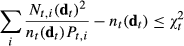
The most widely used goodness‐of‐fit test is the chi‐square test (see, e.g., Chernoff and Lehmann 1954) with the statistical test

\sum_{i} \frac{(N_{t, i} (d_{t}) - n_{t} (d_{t}) P_{t, i})^{2}}{n_{t} (d_{t}) P_{t, i}} \leq χ_{t}^{2} t = 1, \dots, T,

where parameter

χ_{t}^{2}

controls how close the observed sample data is to the estimated expected number of observations according to the fitted distribution

(P_{t, i})_{i = 1, \dots, M_{t}}

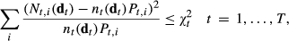
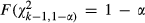
More specifically, suppose that k is the number of bins, c is the number of estimated parameters for the fitted distribution (e.g., c = 2 for normal distributions due to the mean and variance), and consider the null hypothesis

H_{0}

that the observations are independent random samples drawn from the fitted distribution. Chernoff and Lehmann (1954) show that if

H_{0}

is true, the test statistic converges to a distribution function that lies between the distribution functions of chi‐square distributions with k − 1 and k − c − 1 degrees of freedom. Let α denote the significance level, and consider

χ_{k - 1, 1 - α}^{2}

such that

F (χ_{k - 1, 1 - α)}^{2} = 1 - α

, where F(x) is the distribution function of the chi‐square distribution with k − 1 degrees of freedom. It is often recommended that we reject the null hypothesis at the significance level α if the test statistic is greater than

χ_{k - 1, 1 - α}^{2}

(see, e.g., Law and Kelton 2000). In our context,

k = M_{t}

and α, whose interpretation is as above, is given by the decision maker.

Since

P_{t, i}

should define a probability distribution, we have

\sum_{i} P_{t, i} = 1

and

P_{t, i} \geq 0

. Let

P_{t}

denote the vector of

(P_{t, i})_{i}

. The set of distributions that satisfy the chi‐square test is

P_{t} (d_{t}) = {P_{t} | A_{t} P_{t} = b_{t}, \sum_{i} \frac{(N_{t, i} (d_{t}) - n_{t} (d_{t}) P_{t, i})^{2}}{n_{t} (d_{t}) P_{t, i}} \leq χ_{t}^{2}, P_{t} \geq 0} t = 1, \dots, T .

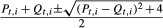
The linear constraints

A_{t} P_{t} = b_{t}

capture at least the fact that

\sum_{i} P_{t, i} = 1

. They can also be used to model more complicated properties of the distribution set, such as constraints on the expected value, any moment, or desired percentiles of the distributions. It is straightforward to establish the compactness of

P_{t} (d_{t})

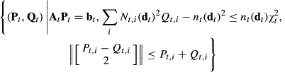
We next give an alternative optimality equation that exploits the structure of Equation . We first provide an alternative characterization of

P_{t} (d_{t})

. We assume that every norm is the Euclidean norm.

Lemma
The set of demand distributions
$P_{t} (d_{t})$
defined in Equation is equivalent to the projection of the set
${(P_{t}, Q_{t}) | A_{t} P_{t} = b_{t}, \sum_{i} N_{t, i} (d_{t})^{2} Q_{t, i} - n_{t} (d_{t})^{2} \leq n_{t} (d_{t}) χ_{t}^{2}, ‖ [\begin{matrix} P_{t, i} - Q_{t, i} \\ 2 \end{matrix}] ‖ \leq P_{t, i} + Q_{t, i}}$

on the space of
$P_{t}$
.

Proof
Since
$\sum_{i} P_{t, i} = 1$
and
$\sum_{i} N_{t, i} (d_{t}) = n_{t} (d_{t})$
, we have
$\begin{matrix} \sum_{i} \frac{(N_{t, i} (d_{t}) - n_{t} (d_{t}) P_{t, i})^{2}}{n_{t} (d_{t}) P_{t, i}} = \sum_{i} \frac{N_{t, i} (d_{t})^{2}}{n_{t} (d_{t}) P_{t, i}} - \sum_{i} 2 N_{t, i} (d_{t}) + \sum_{i} n_{t} (d_{t}) P_{t, i} = \sum_{i} \frac{N_{t, i} (d_{t})^{2}}{n_{t} (d_{t}) P_{t, i}} - n_{t} (d_{t}) . \end{matrix}$

As
$χ_{t}^{2}$
and
$n_{t} (d_{t})$
are finite, we have
$P_{t, i} > 0$
for any i. Therefore,
$\sum_{i} \frac{N_{t, i} (d_{t})^{2}}{n_{t} (d_{t}) P_{t, i}} - n_{t} (d_{t}) \leq χ_{t}^{2}$
is equivalent to
$\sum_{i} N_{t, i} (d_{t})^{2} Q_{t, i} - n_{t} (d_{t})^{2} \leq n_{t} (d_{t}) χ_{t}^{2}, \frac{1}{P_{t, i}} \leq Q_{t, i}, P_{t, i}, Q_{t, i} > 0 .$

Obviously, we have
$\frac{1}{P_{t, i}} \leq Q_{t, i}, P_{t, i}, Q_{t, i} > 0 ⟺ P_{t, i} Q_{t, i} \geq 1, P_{t, i}, Q_{t, i} \geq 0 ⟺ [\begin{matrix} P_{t, i} 11 Q_{t, i} \end{matrix}] ⪰ 0 .$

Note that the eigenvalues of the matrix
$[\begin{matrix} P_{t, i} 11 Q_{t, i} \end{matrix}]$
are
$\frac{P_{t, i} + Q_{t, i} \pm \sqrt{(P_{t, i} - Q_{t, i})^{2} + 4}}{2}$
, and therefore, the positive semidefinite constraint is equivalent to
$\frac{P_{t, i} + Q_{t, i} - \sqrt{(P_{t, i} - Q_{t, i})^{2} + 4}}{2} \geq 0 ⟺ ‖ [\begin{matrix} P_{t, i} - Q_{t, i} \\ 2 \end{matrix}] ‖ \leq P_{t, i} + Q_{t, i},$
which proves the proposition.

Lemma shows that the set
$P_{t} (d_{t})$
can be defined by a set of linear and second‐order cone constraints (see, e.g., Lobo et al. 1998). Note that the second‐order cone constraints are a special class of positive semidefinite constraints, and they have better computational properties than general positive semidefinite constraints. This alternative definition of the set
$P_{t} (d_{t})$
also suggests a compact optimality equation.

Proposition
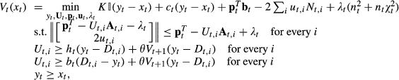
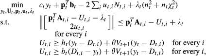
The optimality equation of the robust stochastic model is equivalent to
$\begin{matrix} V_{t} (x_{t}, d_{t}) = \min_{y_{t}, U_{t}, p_{t}, u_{t}, λ_{t}} K I (y_{t} - x_{t}) + c_{t} (y_{t} - x_{t}) + p_{t}^{T} b_{t} - 2 \sum_{i} u_{t, i} N_{t, i} (d_{t}) + λ_{t} (n_{t} (d_{t})^{2} + n_{t} (d_{t}) χ_{t}^{2}) s.t. ‖ [\begin{matrix} p_{t}^{T} - U_{t, i} A_{t, i} - λ_{t} \\ 2 u_{t, i} \end{matrix}] ‖ \leq p_{t}^{T} - U_{t, i} A_{t, i} + λ_{t} for every i U_{t, i} \geq h_{t} (y_{t} - D_{t, i}) + θ V_{t + 1} (y_{t} - D_{t, i}, [d_{t}, D_{t, i}]) for every i U_{t, i} \geq b_{t} (y_{t} - D_{t, i}) + θ V_{t + 1} (y_{t} - D_{t, i}, [d_{t}, D_{t, i}]) for every i y_{t} \geq x_{t}, \end{matrix}$

for any t = 1,…,T.

Proof
Please refer to the Online Supplement.

Note that this is not the standard optimality equation since
$V_{t + 1} (\cdot)$
is present in constraints and not the objective function. We use it later to obtain computationally tractable control policies.
4.1. Computation of (s, S) Levels

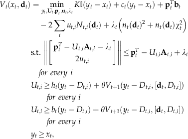
Next, we give a computational approach to compute

s_{t} (d_{t})

and

S_{t} (d_{t})

Theorem 2
Let
$S_{t} (d_{t})$
be an optimal solution to the minimization problem
$\begin{matrix} \min_{y_{t}, U_{t}, p_{t}, u_{t}, λ_{t}} c_{t} y_{t} + p_{t}^{T} b_{t} - 2 \sum_{i} u_{t, i} N_{t, i} (d_{t}) + λ_{t} (n_{t} (d_{t})^{2} + n_{t} (d_{t}) χ_{t}^{2}) s.t. ‖ [\begin{matrix} p_{t}^{T} A_{t, i} - U_{t, i} - λ_{t} 2 u_{t, i} \end{matrix}] ‖ \leq p_{t}^{T} A_{t, i} - U_{t, i} + λ_{t} for every i U_{t, i} \geq h_{t} (y_{t} - D_{t, i}) + θ V_{t + 1} (y_{t} - D_{t, i}, [d_{t}, D_{t, i}]) for every i U_{t, i} \geq b_{t} (D_{t, i} - y_{t}) + θ V_{t + 1} (y_{t} - D_{t, i}, [d_{t}, D_{t, i}]) for every i, \end{matrix}$

and let
$s_{t} (d_{t})$
be the smallest element of the set
${s_{t} (d_{t}) | s_{t} (d_{t}) \leq S_{t} (d_{t}), f_{t} (s_{t}, d_{t}) = f_{t} (S_{t}, d_{t}) + K},$

where
$f_{t} (y_{t}, d_{t})$
is defined by Equation .

A state‐dependent (s, S) policy is optimal for the robust stochastic model with
$P_{t} (d_{t})$
defined by Equation , and the s, S levels are given by
$s_{t} (d_{t})$
and
$S_{t} (d_{t})$
, respectively. If there is no fixed cost, a state‐dependent base‐stock policy is optimal, and the base‐stock level given the realized demand
$d_{t}$
is
$S_{t} (d_{t})$
.

Proof
The minimization problem to calculate
$S_{t} (d_{t})$
follows from the alternative optimality Equation .

Consider the models where the historical data used for period t is independent of the realized demand from periods 1 to t − 1, that is, the number of observations
$N_{t, i}$
in the ith bin and the total number of available observations
$n_{t}$
are constant for any realized demand
$d_{t}$
. Therefore, the set of distributions that satisfy the chi‐square test is defined by
$P_{t} = {P_{t} | A_{t} P_{t} = b_{t}, \sum_{i} \frac{(N_{t, i} - n_{t} P_{t, i})^{2}}{n_{t} P_{t, i}} \leq χ_{t}^{2}, P_{t} \geq 0} t = 1, \dots, T .$

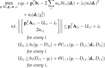
In this case, the optimality equation of the robust model is reduced to
$V_{t} (x_{t}) = \min_{y_{t} \geq x_{t}} \max_{P_{t} \in P_{t}} {\sum_{i} P_{t, i} (C_{t} (x_{t}, y_{t}, D_{t, i}) + θ V_{t + 1} (y_{t} - D_{t, i}))} t = 1, \dots, T,$
where
$P_{t}$
and
$C_{t} (x_{t}, y_{t}, D_{t, i})$
are defined by Equations and , respectively.

Alternatively, it can be written as
$\begin{matrix} V_{t} (x_{t}) & = \min_{y_{t}, U_{t}, p_{t}, u_{t}, λ_{t}} K I (y_{t} - x_{t}) + c_{t} (y_{t} - x_{t}) + p_{t}^{T} b_{t} - 2 \sum_{i} u_{t, i} N_{t, i} + λ_{t} (n_{t}^{2} + n_{t} χ_{t}^{2}) \\ s.t. ‖ [\begin{matrix} p_{t}^{T} - U_{t, i} A_{t, i} - λ_{t} \\ 2 u_{t, i} \end{matrix}] ‖ \leq p_{t}^{T} - U_{t, i} A_{t, i} + λ_{t} for every i \\ U_{t, i} \geq h_{t} (y_{t} - D_{t, i}) + θ V_{t + 1} (y_{t} - D_{t, i}) for every i \\ U_{t, i} \geq b_{t} (D_{t, i} - y_{t}) + θ V_{t + 1} (y_{t} - D_{t, i}) for every i \\ y_{t} \geq x_{t}, \end{matrix}$
for any t = 1,…,T.

The corresponding optimal (s, S) policy levels are also independent of the realized demand
$d_{t}$
.

Theorem 3
The (s, S) policy is optimal for the robust stochastic model (11). In particular, let
$S_{t}$
be the optimal solution to the minimization problem
$\begin{matrix} \min_{y_{t}, U_{t}, p_{t}, u_{t}, λ_{t}} & c_{t} y_{t} + p_{t}^{T} b_{t} - 2 \sum_{i} u_{t, i} N_{t, i} + λ_{t} (n_{t}^{2} + n_{t} χ_{t}^{2}) \\ s.t. & ‖ [\begin{matrix} p_{t}^{T} A_{t, i} - U_{t, i} - λ_{t} \\ 2 u_{t, i} \end{matrix}] ‖ \leq p_{t}^{T} A_{t, i} - U_{t, i} + λ_{t} \\ for every i \\ U_{t, i} \geq h_{t} (y_{t} ‐ D_{t, i}) + θ V_{t + 1} (y_{t} ‐ D_{t, i}) for every i \\ U_{t, i} \geq b_{t} (D_{t, i} ‐ y_{t}) + θ V_{t + 1} (y_{t} ‐ D_{t, i}) for every i, \end{matrix}$

and let
$s_{t}$
be the smallest element of the set
${s_{t} | s_{t} \leq S_{t}, f_{t} (s_{t}) = f_{t} (S_{t}) + K},$

where
$\begin{matrix} f_{t} (y_{t}) & = c_{t} y_{t} + \max_{P_{t} \in P_{t}} \sum_{i} P_{t, i} [h_{t} (y_{t} - D_{t, i})^{+} + b_{t} (y_{t} - D_{t, i})^{-} \\ + θ V_{t + 1} (y_{t} - D_{t, i})] . \end{matrix}$

The policy is to order
$S_{t} - x_{t}$
units in period t if
$x_{t} \leq s_{t}$
, and no order is placed otherwise.

Without fixed procurement cost, a base‐stock policy is optimal, that is,
$S_{t} - x_{t}$
units are ordered in period t if
$x_{t} \leq S_{t}$
, and no order is placed otherwise.

4.2. Summary of Convergence Results

In this subsection, we explore the case of the bins in the histogram being defined by distinctive values in the sample data, and we study the performance of the robust model when the number of samples increases. The important results are summarized in the remaining part of this subsection, and the details of the analysis are presented in Appendix A.

The majority of the results are built on the following convergence property: as

χ_{t}^{2}

approaches to 0, the cost‐to‐go function

V_{t} (x_{t}, d_{t})

of the robust model converges to the corresponding cost‐to‐go function of the stochastic model where the demand distributions follow the empirical distribution defined by the histogram (cf. Proposition A1).

If there exists no fixed procurement, then based on Proposition , if (i)

χ_{t}^{2}

converges to 0 and (ii) the empirical distribution functions converge pointwise to the true distribution function, then the cost‐to‐go function of the robust model converges to that of the stochastic model with the true demand distribution (cf. Proposition ). In particular, if the demand distributions for each time period follow independent continuous distributions, the convergence of the robust model holds as long as the sample size approaches infinity and

χ_{t}^{2}

converges to 0 (cf. Corollary ).

For the models with both fixed and variable procurement cost, we consider the case where the demands follow a discrete distribution over a finite set. Similar to Proposition , the cost‐to‐go function of the robust model converges to that of the stochastic model with the true demand distribution under the conditions that (i)

χ_{t}^{2}

converges to 0 and (ii) the empirical distribution converges to the true distribution (cf. Proposition ). We have also identified a condition under which the convergence holds without

χ_{t}^{2}

approaching 0 (cf. Proposition ). Moreover, if the demand distributions are independent across different periods, as long as the sample size goes to infinity, the cost‐to‐go function of the robust model converges to that of the stochastic model with the true demand distribution, and the rate of convergence is

O (1 / \sqrt{k})

, where k denotes the sample size (cf. Corollary ).

The convergence study not only provides the asymptotic performance of the robust model when the sample size approaches infinitely but also guarantees that the robust models with small bin sizes and small

χ^{2}

values perform well in the presence of a significant number of samples.

5. Computational Results

In this section, we describe computational experiments and present numerical results to support the effectiveness of the minimax robust model based on the chi‐square test. In particular, the robust model proposed in section 4 is compared with (i) the approach which first fits the historical data and then solves the inventory optimization model using the fitted distribution and (ii) the robust model based on Delage and Ye (2010). These two comparisons are presented in the following two subsections, respectively.

5.1. Comparison with Separated Data‐Fitting and Inventory Optimization

As we have mentioned in the previous sections, the traditional approach is to fit the historical data with a distribution and then apply stochastic inventory optimization using the fitted distribution. The main objective of our experiments is to compare performances of this separated approach and the studied minimax robust model with respect to optimality and robustness. At the same time, we would like to assess sensitivity of the robust model to the choices of the bin sizes and

χ^{2}

parameters and provide an empirical approach to choosing these values.

We consider inventory control problems without fixed ordering costs. Following the notation in the previous sections, we let T denote the planning horizon and

c_{t}

h_{t}

b_{t}

denote the variable order cost, unit inventory holding cost, and backorder cost for any period t, t = 1,…,T, respectively. The demand distributions for any period t are assumed to be i.i.d. In the robust model, we restrict ourselves to the case of equal bin sizes, and these, together with

χ^{2}

, are the same for every period in the planning horizon. To simplify the notation, pair

‹ ϵ, χ^{2} ›

denotes the choice of the bin size ε and

χ^{2}

in the robust model.

The procedure of the computational experiments is as follows.

Step 1.
Suppose that the underlying demand distribution has support
${0, 1, \dots, \bar{D}}$
. We randomly generate a distribution among all distributions whose support is a subset of
${0, 1, \dots, \bar{D}}$
. In particular, we pick distribution
$p_{i} = P ({\tilde{D}}_{t} = i) = \frac{U_{i}}{\sum_{i = 0}^{\bar{D}} U_{i}},$
for any
$i = 0, 1, \dots, \bar{D}$
, where
$U_{i}$
for all i are i.i.d. random variables uniformly distributed in the interval [0,1]. We refer to the distribution
$p = {p_{i}}_{i}$
as the true distribution.
Step 2.
Generate n random samples according to the true distribution selected in Step 1.
Step 3.
Fit the samples obtained in Step 2 using Crystal Ball and then choose the l best‐fitted distributions according to the
$χ^{2}$
goodness‐of‐fit statistic.
Step 4.
Solve the standard stochastic inventory control problem with distributions generated in Steps 1 and 3.
Step 5.
Solve the robust inventory control model using a set of bin size and
$χ^{2}$
combinations.
Step 6.
Evaluate the total expected cost with respect to the true distribution p corresponding to the policies of the stochastic models and robust models computed in Steps 4 and 5. We use this step to investigate the optimality of the robust models.
Step 7.
The n samples generated in Step 2 define the empirical distribution
$\hat{p}$
such that
${\hat{p}}_{i} = \frac{the number of times value iappears in the nsamples}{n}$
for any
$i = 0, 1, \dots, \bar{D}$
. Let
$δ = p - \hat{p}$
. We generate m random permutations of vector δ and denote the jth permutation of the coordinates by
$δ^{j}$
. Vector
${\hat{p}}^{j} = \hat{p} + δ^{j}$
also defines a distribution. Note that
${\hat{p}}^{j}$
is equal to p if
$δ^{j} = δ$
, that is, when
$δ^{j}$
is not permuted.

For each distribution defined by vector
${\hat{p}}^{j}$
, we can evaluate the corresponding cost for each policy computed in Steps 4 and 5. Therefore, we obtain m costs for each policy and we report the conditional value‐at‐risk (CVaR) at the 5% level of the m costs for each policy. The purpose of this step is to understand the robustness of different approaches.

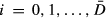
Let us consider a 10‐period problem. The support for the demand distribution is assumed to be the set {0,1,…,29}, that is,
$\bar{D} = 29$
. The cost parameters
$c_{t}$
,
$h_{t}$
, and
$b_{t}$
are generated independently according to uniform distributions within the intervals [12, 15], [2, 5], and [22, 25], respectively. Following the computational procedure, we first draw n = 20 samples from the selected true distribution. Fitting the samples using Crystal Ball, the three best‐fitted distributions according to the chi‐square values are negative binomial, Poisson, and beta. The true distribution p, sample frequency
$\hat{p}$
, and the three distributions are shown in Figure .

Figure 1
True Distribution, Frequency, and Fitted Distributions With 20 Samples

In Steps 4 and 5 of our procedure, we compute the base‐stock levels corresponding to different models: the stochastic model using the true distribution, the stochastic model using the three best‐fitted distributions, and robust models with different bin size and
$χ^{2}$
value combinations. In particular, the following set of bin size and
$χ^{2}$
value combinations are considered: ‹3,1›, ‹3,3›, ‹3,5›, ‹5,1›, ‹5,3›, ‹5,5›.

As stated in our analysis, the robust model picks the demand distribution based on the on‐hand inventory after the order is received, that is, the order‐up‐to level
$y_{t}$
. Although we use the same histogram in each period, the demand distribution returned by the robust model depends also on t. We use the robust model with the bin size/
$χ^{2}$
value ‹3,3› to illustrate these properties.

In Figures and and Table , we use a simple representative sample of cost parameters. Figure shows the robust distributions for the last period t = 10 and the first period t = 1 when the inventory levels after receiving the order
$y_{t}$
are 0 and 20, respectively. For both periods, the distributions returned by the robust model for
$y_{t} = 20$
have lower probabilities in the region 15–26 than those for
$y_{t} = 0$
. The intuition behind this observation is that the robust model picks a demand distribution maximizing the expected cost. For any possible value of the demand, we incur a certain cost corresponding to
$U_{t, i} (y_{t}, d_{t})$
defined in Equation . Therefore, the robust model chooses a lower probability for demand values with lower costs. Value
$y_{t} = 20$
is very close to the demand when the demand falls in the region 15–26. The amount we over‐ or under‐order is low, and, hence, the corresponding over‐ or under‐order cost is also low. Therefore, the corresponding costs associated with the demand values are lower than the costs corresponding to other demand values. As a result, the robust model assigns lower probabilities in these regions compared with the case when
$y_{t} = 0$
.

Figure 2
Demand Distributions Returned by the Robust Model With Bin Size = 3 and
$χ^{2} = 3$

Figure 3
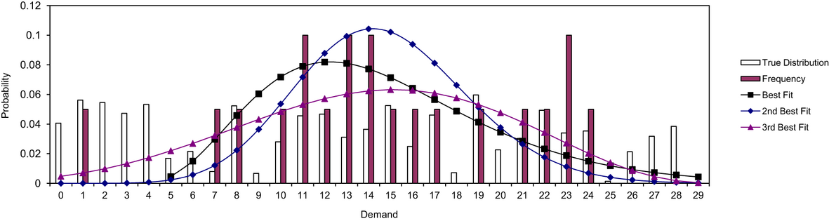
Base‐Stock Levels Computed Using Different Models

Table 1
Performance of Different Models for the Instance in Figure

Stochastic models Robust models

True dist Best fit Second best fit Third best fit ‹3,1› ‹3,3› ‹3,5› ‹5,1 or 3 or 5›

Cost 1 1.0595 1.1834 1.0582 1.0415 1.0211 1.0249 1.1511

CVaR 1 1.0486 1.1802 1.0511 1.0356 0.9774 0.9739 1.1662

If we compare the robust distributions when
$y_{t} = 20$
for period 10 and period 1, we observe that the probability for period 10 is higher for small demand values. This can also be explained by the tradeoff between the over‐ and under‐order costs. In the last period, the over‐order cost is
$c_{10} + h_{10}$
and the under‐order cost is
$b_{10}$
since we set
$V_{T + 1} (\cdot) = 0$
. For any earlier period t < 10, the over‐order costs are significantly lower as we can carry the inventory to the next period and save the order cost
$c_{t}$
, but the under‐order cost is
$b_{t} + c_{t + 1}$
since we not only pay the backorder cost but also procure the product in period t + 1 to satisfy the unmet demand in period t. When
$y_{t} = 20$
, we pay the over‐order costs when the demands are low (e.g., in the region 0–11), and the under‐order costs are incurred when the demand are high (e.g., in the region 21–26). As the over‐order costs are higher and the under‐order costs are lower in the last period, it implies that the ratio between the costs for low demands and the costs for high demands is greater in period 10 than period 1. This is the reason why the robust model assigns higher probabilities for low demands in period 10.

On the other hand, the robust distributions when
$y_{t} = 0$
are almost the same for the two periods with t = 10 and t = 1. In this case, we only have the under‐order cost no matter if the demand is high or low. Although the under‐order cost is higher in period 1 than period 10, the ratios between the costs for low and high demands are almost the same for periods 1 and 10. Therefore, the worst case distributions are similar for these two periods.

The base‐stock levels computed in Steps 4 and 5 are displayed in Figure . For any of the stochastic or robust models, the base‐stock level for period 10 is significantly lower than the remaining periods. As explained before, this is caused by the fact that the over‐order cost is much higher while the under‐order cost is lower in period 10 because of
$V_{T = 1} (\cdot) = 0$
, and thus, we should order less in that period. In addition, the base‐stock level for period 4 is slightly lower for most of the models since period 4 has the highest order and inventory holding cost, while its backorder cost is relatively low.

For the three robust models with the bin‐size 3, the base‐stock levels are nondecreasing with respect to the
$χ^{2}$
value, since the sets of distributions are inclusion‐wise increasing in the
$χ^{2}$
value. In our instances, the backorder cost is much higher than the inventory holding cost. Intuitively, the worst case distribution should assign higher probabilities for high‐demand values. Therefore, the larger the
$χ^{2}$
value is, the higher the probabilities for high‐demand values in the worst case distribution, and, hence, we should order more to minimize the worst case expected cost. As a result, the base‐stock levels are higher for the robust models with greater
$χ^{2}$
values. However, if we set the bin size to 5 for the robust models, the base‐stock levels are the same when the
$χ^{2}$
values are equal to 1, 3, and 5. This observation indicates that the base‐stock levels are less sensitive to the
$χ^{2}$
values when we have larger bins.

We use Steps 6 and 7 to understand the performance of different models. The results are summarized in Table . The first four columns correspond to the results for the stochastic models using true distribution p and the three best‐fitted distributions, respectively. The next four columns show the results for the robust models. Note that the last column corresponds to the robust models with bin size 5 and
$χ^{2}$
values 1, 3, and 5. These three robust models have the same performance for this example as they have the same base‐stock levels. We show the expected cost for different models with respect to the true distribution in the first line, which corresponds to the output of Step 6. In the second line, we report the output of Step 7, that is, the CVaR at 5% level for the costs of m = 1000 distributions generated by
$\hat{p}$
plus random permutations of
$p - \hat{p}$
. For the purpose of comparison, the numbers in Table are calculated by subtracting the cycle stock order cost, that is,
$(\sum_{t = 1}^{T} c_{t}) (\sum_{i = 1}^{\bar{D}} {ip}_{i})$
, from the original cost or CVaR, and normalizing with respect to that of the stochastic model using true distribution.

Obviously, the stochastic model using the true distribution gives the lowest expected cost. The output of Step 7, CVaR, also indicates that this model is robust with respect to perturbations in the input distribution as it has the third lowest CVaR, which is only 2.61% higher than the lowest CVaR.

For the three stochastic models using fitted distributions, the models using the first and third best‐fitted distributions have a very similar performance. The best‐fit case has the best performance among the fitted stochastic models as its CVaR is 0.25% better than the third best‐fit stochastic model, and the cost is only 0.13% higher than that. The performance of the model using the second best distribution is much worse compared with the other two. Its cost and CVaR values are at least 12% higher than those of the remaining two models.

The three robust models with bin size 3 outperform all of the stochastic models using fitted distributions in terms of both optimality (cost) and robustness (CVaR). The robust models with bin size 5 also have better values of the cost and CVaR than the stochastic model using the second best‐fitted distribution. In particular, the robust models with bin size/
$χ^{2}$
value combinations of ‹3,3› and ‹3,5› are significantly better than the stochastic models using fitted distributions. They reduce the cost by more than 3% and CVaR by more than 7% when comparing with the fitted stochastic models. Among the robust models, we prefer the model with bin size/
$χ^{2}$
value combination ‹3,3›, since it improves the cost by 0.38% at the price of a 0.35% increase in CVaR.

There are mainly two reasons why the robust model outperforms the stochastic model with the best‐fit distribution. First, the sample size is relatively small, and hence, the fitted distributions could be significantly different from the true distribution. The robust model, on the other hand, recognizes the difference between the samples and the true distribution and corrects the error by considering a set of distributions close to the empirical histogram. Second, although Crystal Ball considers 16 families of commonly used parametric distributions, it is still possible that the true distribution does not follow any one of these 16 families of distributions. In fact, most distribution encountered in practice cannot be described using parametric families such as the uniform or Poisson distributions. Therefore, as long as the true distribution does not belong to any parametric family of distributions, the best‐fit distribution does not match the true distribution even if the sample size goes to infinity. The robust approach based on the chi‐squared test, which does not make any assumption regarding the parametric family of the underlying distribution, is much more flexible in this perspective.

Next, we repeated the experiment 10 times from Step 1 to Step 7, that is, each time with a different true distribution, demand data, and cost parameters. Table shows the average and standard deviation of the cost and CVaR values for the 10 data samples for the stochastic model using the true distribution, the stochastic model using the best‐fitted distribution, as well as the six robust models already considered. All robust models have lower average and standard deviation of cost and CVaR compared with the stochastic model using the best‐fitted distribution. In terms of both optimality (cost) and robustness (CVaR), the performance of our robust models is better on average (smaller average) and more stable (smaller standard deviation) than the stochastic model using the best‐fitted distribution.

Table 2
Performance of Different Models in 10 Instances

Stochastic models Robust models

True dist Best fit ‹3,1› ‹3,3› ‹3,5› ‹5,1› ‹5,3› ‹5,5›

Cost

Average 1 1.0902 1.0412 1.0361 1.0499 1.0725 1.0597 1.0570

SD 0 0.0893 0.0210 0.0302 0.0330 0.0736 0.0511 0.0519

CVaR

Average 1 1.0894 1.0014 0.9745 0.9746 1.0648 1.0281 1.0212

SD 0 0.1142 0.0507 0.0327 0.0355 0.0917 0.0639 0.0618

The robust models with bin size 3 have lower values of average and standard deviation of both measures than the robust models with bin size 5. Moreover, the robust models with higher
$χ^{2}$
values, for example, when
$χ^{2}$
is set to 3 or 5, have lower CVaR than those with
$χ^{2}$
values set to 1. This observation agrees with our understanding that increasing
$χ^{2}$
values can improve the robustness of the models. However, it may also affect the cost of the models; for example, the average cost for the ‹3,5› robust model is 0.8% higher than that of the ‹3,1› robust model.

The robust model with bin size 3 and
$χ^{2}$
value 3 has the lowest average cost, lowest CVaR, and lowest standard deviation of CVaR among all robust models, and its standard deviation of the cost is the second lowest. This agrees with our suggestion drawn from Figure : the robust model with bin size/
$χ^{2}$
value combination ‹3,3› should be the best among the robust models.

Figure shows the cost and CVaR values for the stochastic model using the best‐fitted distribution and the ‹3,3› robust model in each of the 10 instances. The cost values of the ‹3,3› robust model are at least 7.5% lower than the stochastic model with the best‐fitted distribution for instances 5, 8, 9, and 10. The improvement in instances 9 and 10 even exceeds 20%. The cost values of instances 2 and 3 are almost the same for both models. Instance 7 is the only case where the cost of the robust model is more than 2% (2.04% to be exact) higher than the cost of the stochastic model.

Figure 4
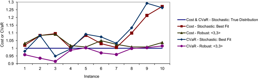
The Stochastic Model Using Best‐Fitted Distribution vs. the Robust Model With Parameters ‹3,3› for 10 Instances

The values of CVaR for the robust model are < 1 for 7 of the 10 instances, they are very close to 1 (at most 0.04% higher than one) for the other two instances, and the largest value is 1.0150. On the other hand, the values of CVaR for the stochastic model with the best‐fitted distribution are < 1 only for three instances and the largest value is 1.2923. We conclude that the ‹3,3› robust model is much more robust compared with the stochastic model using the true distribution.

To understand the sensitivity of different models with respect to the number of samples drawn from the true distribution, we ran 10 additional experiments in which we generated n = 40 samples from the true distribution in Step 2.

Table summarizes the main statistics of the stochastic model using the best‐fitted distribution and our robust models. Similar to the result in Table where we have 20 samples from the true distribution, all the robust models outperform the stochastic model with the best‐fitted distribution in both the average and standard deviation of the two measures.

Table 3
Performance of Different Models for 10 Instances and 40 Samples

Stochastic models Robust models

True dist Best fit ‹3,1› ‹3,3› ‹3,5› ‹5,1› ‹5,3› ‹5,5›

Cost

Average 1 1.0749 1.0278 1.0223 1.0364 1.0457 1.0317 1.0304

SD 0 0.0500 0.0232 0.0262 0.0346 0.0353 0.0297 0.0297

CVaR

Average 1 1.0824 1.0146 0.9904 0.9832 1.0544 1.0170 1.0092

SD 0 0.0768 0.0415 0.0272 0.0216 0.0445 0.0165 0.0126

As expected, the average cost of all robust models and the best‐fit stochastic model improve when the sample size increases from 20 to 40. The robust models with bin size 5 have a slightly greater improvement than the remaining models. For the other three statistics, we also observe improvements for the stochastic model using the best‐fitted distribution as well as the robust models with bin size 5 when the sample size is increased to 40. Again, the robust models with bin size 5 show slightly better improvements in these statistics.

If we compare the robust models with different bin sizes, those with bin size 3 still perform better than those with bin size 5. However, compared with the case of 20 samples, the differences are slightly smaller for all statistics, which suggests that the robust models with bin size 5 improve faster as the sample size increases. Similar to the experiments with 20 samples, the increase in
$χ^{2}$
values also helps to improve the robustness of the models, which is measured by CVaR. The improvements in robustness as
$χ^{2}$
values increase are more significant for 40‐sample experiments than those with 20 samples. In addition, the increased
$χ^{2}$
may also increase the cost; for example, the average cost increases from 1.0278 to 1.0364 if we increase the
$χ^{2}$
value from 1 to 5 for the robust models with bin size 3.

The robust model with parameters ‹3,3› has the lowest average cost, the second lowest average CVaR, and the second lowest standard deviation of the cost. Besides, its standard deviation of CVaR is < 3%. We still consider it as the most efficient model among all the robust models and the stochastic model using the best‐fitted distribution.

To summarize the numerical results, the computational experiments show that the robust models outperform the stochastic models using fitted distributions in terms of both optimality and robustness. The robust models with a lower bin size perform better than those with a larger bin size, but an increase in sample size may decrease the difference in performance caused by the choice of the bin size. In addition, a higher
$χ^{2}$
value helps increase the robustness, but it may sacrifice the cost of the robust models.
5.2. Comparison with the Robust Model Based on Delage and Ye (2010)

	Stochastic models	Robust models
Cost
Average	1	1.0902	1.0412	1.0361	1.0499	1.0725	1.0597	1.0570
SD	0	0.0893	0.0210	0.0302	0.0330	0.0736	0.0511	0.0519
CVaR
Average	1	1.0894	1.0014	0.9745	0.9746	1.0648	1.0281	1.0212
SD	0	0.1142	0.0507	0.0327	0.0355	0.0917	0.0639	0.0618

	Stochastic models	Robust models
Cost
Average	1	1.0749	1.0278	1.0223	1.0364	1.0457	1.0317	1.0304
SD	0	0.0500	0.0232	0.0262	0.0346	0.0353	0.0297	0.0297
CVaR
Average	1	1.0824	1.0146	0.9904	0.9832	1.0544	1.0170	1.0092
SD	0	0.0768	0.0415	0.0272	0.0216	0.0445	0.0165	0.0126

Delage and Ye (2010) propose a robust formulation for single‐stage optimization problems, which minimizes the worst‐case expectation over a set of distributions defined by the estimates of the mean

μ_{0}

and variance‐covariance matrix

Σ_{0}

of the underlying distribution. Let ξ denote the κ‐dimensional vector of random parameters in the optimization problem and

f_{ξ}

the distribution of ξ. The set of distributions considered in Delage and Ye (2010) is

D = {f_{ξ} \in M | P (ξ \in S) = 1, (E [ξ] - μ_{0}^{T}) Σ_{0}^{- 1} (E [ξ] - μ_{0}^{T}) \leq γ_{1}, E [(ξ - μ_{0}) (ξ - μ_{0})^{T}] γ_{2} Σ_{0}},

where

M

is the set of probability measures in

R^{κ}

S \subseteq R^{κ}

is a closed convex set containing the support of ξ, and

γ_{1} \geq 0

and

γ_{2} \geq 1

are two parameters controlling the size of

D

. When

μ_{0}

and

Σ_{0}

correspond to the sample mean and variance, Delage and Ye (2010) identify certain conditions for

γ_{1}

γ_{2}

, and the sample size under which the probability that the distribution of ξ lies in

D

is greater than a given confidence level.

Obviously, the set defined in Equation is also applicable to the robust inventory model discussed in section 2. Similarly to the computational settings in the previous part, suppose that the demand distribution is stationary and we have n samples drawn from the true distribution. Let

\hat{μ}

and

{\hat{σ}}^{2}

denote the sample mean and variance, respectively. If the support of

{\tilde{D}}_{t}

is contained in the set

{0, 1 ., \dots, \bar{D}}

for any t, the set of distributions in Equation can be written as follows:

P^{DY} = {P | \sum_{i = 0}^{\bar{D}} P_{i} = 1, - {\hat{σ}}_{t} \sqrt{γ_{1}} \leq \sum_{i = 0}^{\bar{D}} i P_{i} - \hat{μ} \leq \hat{σ} \sqrt{γ_{1}}, \sum_{i = 0}^{\bar{D}} (i - \hat{μ})^{2} P_{i} \leq γ_{2} {\hat{σ}}^{2}, P \geq 0} .

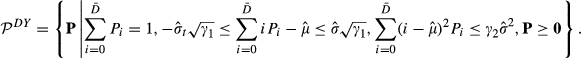
Replacing

P_{t} (d_{t})

in Equation by

P^{DY}

, we obtain a minimax robust inventory model. Without a fixed ordering cost, the optimal policy is a base‐stock policy, and the base‐stock levels can be computed in a fashion similar to Theorem . Next, we apply this approach to all the instances generated in section 1, and we use Steps 6 and 7 in section 5.1 to evaluate its performance.

An important issue when applying the robust model based on Delage and Ye (2010) is to determine the values of the parameters

γ_{1}

and

γ_{2}

. We choose 10 pairs of

γ_{1}

and

γ_{2}

using a statistical analysis similar to that in the computational experiments in Delage and Ye (2010). In particular, we generated 1000 distributions as described in Step 1 in section 5.1. Each of these distributions is referred to as the jth distribution, j = 1,…,1000. The values of

γ_{1}

and

γ_{2}

are selected so that set

P^{DY}

in Equation defined by

γ_{1}

γ_{2}

, and the mean and variance of the jth distribution contains the mean and variance of the (j + 1)th distribution with a confidence level

c^{DY}

. Table displays the values of

γ_{1}

and

γ_{2}

for different

c^{DY}

used in the computation.

Table 4
Values of
$γ_{1}$
and
$γ_{2}$
for the Robust Model Based on Delage and Ye (2010)

$c^{DY}$ 99% 90% 80% 70% 60% 50% 40% 30% 20% 10%

$γ_{1}$
0.1655 0.0668 0.0426 0.0261 0.0182 0.0115 0.0059 0.0028 0.0010 0.0002

$γ_{2}$
1.3572 1.1916 1.1220 1.07450 1.0395 1.0034 0.9693 0.9315 0.8897 0.8381

$c^{DY}$	99%	90%	80%	70%	60%	50%	40%	30%	20%	10%
$γ_{1}$	0.1655	0.0668	0.0426	0.0261	0.0182	0.0115	0.0059	0.0028	0.0010	0.0002
$γ_{2}$	1.3572	1.1916	1.1220	1.07450	1.0395	1.0034	0.9693	0.9315	0.8897	0.8381

For the example discussed in Figure , we apply the robust model based on Delage and Ye for different

γ_{1}

and

γ_{2}

corresponding to the values of

c^{DY}

in Table . Table shows the normalized cost with respect to the true distribution in the second row, and in the third row, the values are the CVaR at 5% level of the costs out of 1000 distributions generated by permutations described in Step 7 of section 5.1.

Table 5

Performance of the Robust Model Based on Delage and Ye (2010) for the Instance in Figure

$c^{DY}$	99%	90%	80%	70%	60%	50%	40%	30%	20%	10%
Cost	1.2142	1.1505	1.1403	1.1352	1.1191	1.1206	1.1122	1.1003	1.0951	1.0868
CVaR	1.0693	1.0461	1.0423	1.0421	1.0380	1.0425	1.0385	1.0385	1.0550	1.0600

In general, the expected cost, which measures the optimality of the model, is decreasing in the confidence level

c^{DY}

, which is expected since the parameters

γ_{1}

and

γ_{2}

, and hence the size of the distributional set, are decreasing in

c^{DY}

. However, the value of CVaR, which measures the robustness of the model, is not increasing in

c^{DY}

. The largest CVaR is obtained when

c^{DY} = 99 %

, which implies that the corresponding distributional set is too large compared with the set of distributions generated by the permutations.

Compared with Table , for most parameters, except for

c^{DY} = 99 %

, the robust model based on Delage and Ye (2010) has lower expected cost and CVaR than our robust model with bin size 5. However, our model with bin size 3 outperforms all results shown in Table . In particular, the performance measures for the ‹3,3› robust model are 1.0211 and 0.9774, respectively, while the lowest expected cost for the model based on Delage and Ye (2010) is 1.0868 (when

c^{DY} = 10 %

) and the lowest CVaR is 1.0380 (when

c^{DY} = 60 %

The robust model based on Delage and Ye (2010) with parameters in Table is also applied to the 20‐ and 40‐sample instances in Tables and . The statistics corresponding to these are presented in Tables and , respectively.

Table 6

Performance of the Robust Model Based on Delage and Ye (2010) for the 20‐Sample Instances in Table

$c^{DY}$	99%	90%	80%	70%	60%	50%	40%	30%	20%	10%
Cost average	1.135	1.125	1.122	1.115	1.117	1.114	1.110	1.112	1.114	1.114
Cost Std. Dev.	0.049	0.052	0.050	0.047	0.045	0.047	0.045	0.053	0.061	0.064
CVaR average	0.957	0.953	0.953	0.951	0.955	0.956	0.957	0.962	0.965	0.969
CVaR Std. Dev.	0.119	0.115	0.115	0.115	0.120	0.122	0.123	0.130	0.134	0.137

Table 7

Performance of the Robust Model Based on Delage and Ye (2010) for the 40‐Sample Instances in Table

$c^{DY}$	99%	90%	80%	70%	60%	50%	40%	30%	20%	10%
Cost average	1.144	1.130	1.126	1.118	1.115	1.109	1.106	1.103	1.100	1.100
Cost Std. Dev.	0.037	0.031	0.030	0.029	0.027	0.027	0.028	0.026	0.025	0.025
CVaR average	1.009	1.004	1.002	1.001	1.001	1.000	1.000	1.002	1.001	1.005
CVaR Std. Dev.	0.067	0.066	0.065	0.064	0.064	0.063	0.062	0.063	0.061	0.069

First, we compare the performance of our robust model in section 4 with the robust model based on Delage and Ye (2010) for the 20‐sample instances. The average cost of the latter is from 1.110 to 1.135 while the corresponding cost in Table is less than 1.073. On the other hand, the model based on Delage and Ye (2010) has lower average CVaR, which varies from 0.951 to 0.969, than our robust model, whose average CVaR is from 0.975 to 1.065. As for the standard deviations, our robust model has a lower standard deviation in CVaR, and its standard deviation in cost is comparable to the model based on Delage and Ye (2010).

We now discuss the 40‐sample instances. The average cost of the model based on Delage and Ye (2010) is almost the same as the 20‐sample instances, but these statistics of our robust model are on average 1.9% lower in the 20‐sample instances. Moreover, our robust model has similar values of CVaR for both 20‐ and 40‐sample instances, while the CVaR of the robust model based on Delage and Ye (2010) increases 4.6% on average when the sample size increases to 40. The two types of robust models have similar standard deviations in cost, but our robust model has a lower standard deviation in CVaR.

The numerical results indicate that our robust model outperforms with respect to the solution quality, which is mainly due to the distributional set derived from the chi‐square test carrying more information about the shape of the distribution compared with the distributional set Equation defined only by the sample mean and variance. The model based on Delage and Ye (2010) is more robust, but the difference in robustness of these two models decreases as we increase the sample size from 20 to 40.

In addition, we identified that the ‹3,3› robust model based on the chi‐square test has the best performance among all of the six combinations of the parameters. For 20‐sample instances, its average cost is 7.3% lower than the lowest cost for the model based on Delage and Ye (2010) (when

c^{DY} = 40 %

) and the corresponding average CVaR is only 2.3% higher than the lowest CVaR of that model (when

c^{DY} = 70 %

). For 40‐sample instances, the average cost and CVaR of the ‹3,3› robust model are lower than the lowest values of the model based on Delage and Ye (2010) (achieved when

c^{DY} = 10 %

and

c^{DY} = 50 %

, respectively) by 7.8% and 1.0%, respectively. We conclude that the ‹3,3› robust model achieves a better tradeoff between optimality and robustness than the model based on Delage and Ye (2010).

6. Conclusions and Extensions

In this study, we propose a robust stochastic model for the multi‐period lot‐sizing problem, in which the demand distribution is unknown and the only available information is historical data. The convergence results for the chi‐square test based models suggest that the solutions to the robust approach are very close to the optimal stochastic programming solutions when the sample size is sufficiently large. When the sample size is relatively small, the extensive numerical results show that the robust model still obtains a close‐to‐optimal solution whose performance is insensitive to the disturbances in demand distributions. This robust framework based on historical data can be extended to many more general finite‐horizon dynamic programming problems, and the convergence properties can also be extended to more general problems.

Although we consider backorder models, most of our results can be extended to lost‐sales models. In particular, for lost‐sales models with only linear procurement cost and under the same technical assumptions, the optimal policy under the robust model is a state‐dependent base‐stock policy.

Footnotes

Appendix A.

Acknowledgments

The authors thank the senior editor and two anonymous referees for their comments to improve the paper. The authors were supported by NSF contract CMMI‐0758069, NASA's Interplanetary Supply Chain Management and Logistics Architectures project, Masdar Institute of Science and Technology (MIST), and grants from Ford, GE, and SAP. The last author was also supported by Hong Kong RGC GRF grant 717111.

1

Note that here we drop subscript t to simplify the notation.

2

{\hat{p}}^{j}

contains any negative component, we set

{\hat{p}}^{j}

to be the positive part of

{\hat{p}}^{j}

plus a random permutation of its negative part, and we repeat this process until

{\hat{p}}^{j} \geq 0

3

Given random variable X, the conditional value‐at‐risk at a quantile‐level q is defined as E[X | X < μ] where μ is defined by P(X < μ) = q.

4

In this section, the over‐order (under‐order, respectively) cost includes not only the inventory holding cost

h_{t}

(backorder cost

b_{t}

, respectively) incurred in period t but also the impact of over‐order (under‐order, respectively) in period t based on the cost‐to‐go function

V_{t + 1} (\cdot)

5

In Delage and Ye (), the means and variances are computed from financial market data in 30 consecutive days, and the confidence level is 99% confidence level.

References

Ahmed

Cakmak

Shapiro

. 2007. Coherent risk measures in inventory problems. Eur. J. Oper. Res. 182(1): 226–238.

Ben‐Tal

Nemirovski

. 1998. Robust convex optimization. Math. Oper. Res. 23(4): 769–805.

Ben‐Tal

Nemirovski

. 2000. Robust solutions of linear programming problems contaminated with uncertain data. Math. Program. 88(3): 411–424.

Bertsimas

Sim

. 2003. Robust discrete optimization and network flows. Math. Program. 98(1–3): 49–71.

Bertsimas

Sim

. 2004. The price of robustness. Oper. Res. 52(1): 35–53.

Bertsimas

Thiele

. 2006. A robust optimization approach to inventory theory. Oper. Res. 54(1): 150–168.

Bienstock

Özbay

. 2008. Computing robust basestock levels. Discrete Optim. 5(2): 389–414.

Billingsley

1986. Probability and Measure, 2nd edn. John Wiley and Sons, New York, NY.

Chen

Simchi‐Levi

. 2004. Coordinating inventory control and pricing strategies with random demand and fixed ordering cost: The finite horizon case. Oper. Res. 52(6): 887–896.

10.

Chernoff

Lehmann

E. L.

. 1954. The use of maximum likelihood estimates in

χ^{2}

tests for goodness‐of‐fit. Ann. Math. Statist. 25(3): 579–586.

11.

Delage

. 2010. Distributionally robust optimization under moment uncertainty with application to data‐driven problem. Oper. Res. 58(3): 596–612.

12.

Gallego

Moon

. 1993. The distribution free newsboy problem: Review and extensions. J. Oper. Res. Soc. 44(8): 825–834.

13.

Guan

Miller

A. J.

. 2008. Polynomial‐time algorithms for stochastic uncapacitated lot‐sizing problems. Oper. Res. 56(5): 1172–1183.

14.

Halman

Klabjan

Mostagir

Orlin

Simchi‐Levi

. 2009. A fully polynomial‐time approximation scheme for single‐item stochastic inventory control with discrete demand. Math. Oper. Res. 34(3): 674–685.

15.

Huh

W. T.

Rusmevichientong

. 2009. A nonparametric asymptotic analysis of inventory planning with censored demand. Math. Oper. Res. 34(1): 103–123.

16.

Iglehart

D. L.

1964. The dynamic inventory problem with unknown demand distribution. Manage. Sci. 10(3): 429–440.

17.

Iyengar

G. N.

2005. Robust dynamic programming. Math. Oper. Res. 30(2): 257–280.

18.

Kouvelis

. 1997. Robust Discrete Optimization and Its Applications. Kluwer Academic Publishers, Dordrecht, Germany.

19.

Law

A. M.

Kelton

W. D.

. 2000. Simulation Modeling and Analysis, 3rd edn. McGraw‐Hill, New York, NY.

20.

Liyanage

L. H.

Shanthikumar

J. G.

. 2005. A practical inventory control policy using operational statistics. Oper. Res. Lett. 33(4): 341–348.

21.

Lobo

Vandenberghe

Boyd

Lebret

. 1998. Applications of second‐order cone programming. Linear Algebra Appl. 284(1–3): 193–228.

22.

Natarajan

Sim

Uichancoz

. 2008. Asymmetry and ambiguity in newsvendor models. Working paper, National University of Singapore, Singapore.

23.

Nilim

El Ghaoui

. 2005. Robust control of Markov decision processes with uncertain transition matrices. Oper. Res. 53 (5): 780–798.

24.

Notzon

. 1970. Minimax inventory and queueing models. Technical Report No. 7, Department of Operations Research, Stanford University, Stanford, CA.

25.

Perakis

Roels

. 2008. Regret in the newsvendor model with partial information. Oper. Res. 56(1): 188–203.

26.

Porteus

E. L.

2002. Foundations of Stochastic Inventory Theory. Stanford University Press, Stanford, CA.

27.

Royden

H. L

. 1988. Real Analysis, 3rd edn. Prentice Hall, Englewood Cliffs, NJ.

28.

Scarf

. 1958. A min‐max solution of an inventory problem. Studies in the Mathematical Theory of Inventory and Production. Stanford University Press, Stanford, CA.

29.

Scarf

. 1960. The optimality of (s,S) policies in the dynamic inventory problems. Mathematical Methods in the Social Sciences. Stanford University Press, Stanford, CA.

30.

See

C. T.

Sim

. 2010. Robust approximation to multi‐period inventory management. Oper. Res. 58(3): 583–594.

31.

Soyster

A. L

. 1973. Convex programming with set‐inclusive constraints and applications to inexact linear programming. Oper. Res. 21(5): 1154–1157.

32.

von Neumann

. 1928. Zur theorie der gesellschaftsspiele. Math. Ann. 100: 295–320.

33.

Zipkin

2000. Foundations of Inventory Management. McGraw‐Hill, New York, NY.

	Stochastic models				Robust models
	True dist	Best fit	Second best fit	Third best fit	‹3,1›	‹3,3›	‹3,5›	‹5,1 or 3 or 5›
Cost	1	1.0595	1.1834	1.0582	1.0415	1.0211	1.0249	1.1511
CVaR	1	1.0486	1.1802	1.0511	1.0356	0.9774	0.9739	1.1662

Robust Stochastic Lot‐Sizing by Means of Histograms

Abstract

Keywords

1. Introduction

1.1. Literature Review

2. Formulation of Robust Stochastic Lot‐Sizing

5. Computational Results

5.1. Comparison with Separated Data‐Fitting and Inventory Optimization

Table 4 Values of γ 1 and γ 2 for the Robust Model Based on Delage and Ye (2010) c DY 99% 90% 80% 70% 60% 50% 40% 30% 20% 10% γ 1 0.1655 0.0668 0.0426 0.0261 0.0182 0.0115 0.0059 0.0028 0.0010 0.0002 γ 2 1.3572 1.1916 1.1220 1.07450 1.0395 1.0034 0.9693 0.9315 0.8897 0.8381

Footnotes

Appendix A.

Acknowledgments

1

2

3

4

5

References