Differences in Retail Inventory Investment Behavior During Macroeconomic Shocks: Role of Service Level

Abstract

In this article, we analyze how retailers change their inventory investment behavior in response to macroeconomic shocks. We examine if service level, as measured by the ratio of stockout to inventory holding costs, can explain the differences in observed behavior across retailers. We use data on macroeconomic indicators and quarterly filings of US public retailers from 1985 to 2009 to estimate a dynamic model of short‐ and long‐term impact of macroeconomic shocks on inventory investment. Our results show that retailers with a high service level increase their inventory investment significantly more than those with a low service level during expansion shocks. Conversely, retailers with a low service level curtail their inventory investment significantly more than those with a high service level during periods of economic contractions. Thus, we show that the aggregate change in inventory investment documented in prior macroeconomics research is driven by different sets of retailers, as predicted by newsvendor logic. We draw implications of our findings to retailers as well as their suppliers.

Keywords

inventory investment macroeconomic shocks expansion contraction inventory holding cost stockout cost service level

1. Introduction

Managing supply chain risk is one of the most critical tasks of supply chain managers (Gurnani et al. 2012). The importance of managing supply chain risk is underscored in the pioneering study of Hendricks and Singhal (2005) that demonstrated the large impact of supply demand mismatches on stock market performance. An important factor that contributes to the risk of supply demand mismatch is uncertain economic cycles (Tang 2006).

Macroeconomic shocks can have an especially large impact on the financial performance of retailers. In the United States, the correlation between GDP¹ and retail sales during the period from 1979 to 2009 is 0.98. This high correlation is driven by the increasing contribution of personal consumption expenditure to the overall GDP, which rose from 62.5% in the 1970s to 70% in 2009. Changes in the overall US economy are thus largely driven by changes in consumer spending, which directly affects retail demand. Therefore, retailers actively change their inventory investment in response to economic shocks to avoid costly supply demand mismatches. A long line of research in macroeconomics that has examined the impact of macroeconomic factors on retail inventory has shown that inventory investment moves pro‐cyclically with business cycles (see Blinder and Maccini 1991 for a review of this literature). In other words, inventory investment increases during expansion periods and decreases during contraction periods. This literature has typically examined changes in industry‐level or country‐level inventory and ignored the firm characteristics that moderate inventory investments in the face of macroeconomic shocks. Thus, it remains unclear whether retailers, belonging to the same segment, differ in their inventory investment behavior in the face of macroeconomic shocks and, if so, what factors might explain the differences across those retailers.

Empirical examination of differences in retailers' inventory investment behavior in response to macroeconomic shocks is important for several reasons. First, suppliers to retailers are impacted not only by changes in end‐consumer demand due to macroeconomic shocks but also by changes in retailers' inventory levels. For example, when Procter & Gamble's sales declined in fiscal year 2009, it blamed the decline in consumer demand as well as inventory reductions at retailers as contributing to its financial downturn.^2,3 Therefore, knowledge of how different retailers change their inventory levels during macroeconomic shocks could help their suppliers plan inventory efficiently. Second, retailers benchmark their inventory performance against that of their competitors and other firms in their industry segment to guide their inventory decisions. Understanding differences in inventory investment behavior across retailers in the face of macroeconomic shocks would help benchmark inventory performance during economically turbulent periods. To summarize, identifying differences in inventory investment behavior across retailers during macroeconomic shocks can help improve inventory management of retailers as well as their suppliers.

In this article, we are motivated by the theoretical literature in operations management to examine if stockout costs and inventory holding costs explain differences, if any, in inventory investment behavior across retailers. In the commonly used newsvendor model, the ratio of these two costs determines the optimal service level of retailers. This, in turn, drives the safety stock held by retailers. We expect macroeconomic shocks to affect not only the mean demand faced by retailers but also the standard deviation of demand. Thus, retailers with different service levels could vary in the amounts by which they adjust their safety stock levels when faced with a macroeconomic shock.

We have the following results. First, we find that inventory investment is pro‐cyclical to macroeconomic shocks. On average, retailers increase (decrease) their inventory investment in response to expansion (contraction) shocks. This result compliments similar findings from the macroeconomics literature by extending the results using more disaggregate firm‐level information. Second, and more importantly, we find that there is significant heterogeneity in inventory investment behavior across retailers. Specifically, we find that a 1% unexpected increase in GDP (expansion shock) in a quarter leads to a 1.7% increase in inventory investments by the end of the subsequent quarter for high service level retailers. This is significantly more than the reaction of low service level retailers (0.60%). Conversely, a 1% unexpected decrease in GDP (contraction shock) leads to a 1.3% decrease in inventory investments by the end of the subsequent quarter for low service level retailers. This decrease is significantly more than that of high service level retailers (0.45%). We call these the short‐term impacts of economic shocks. The long‐term impacts, or the total impacts, of expansion shocks on inventory investments for high (low) service level retailers are a 3.1% (1.14%) increase in their inventory investments. The corresponding values for contraction shocks are a 2.26% (0.77%) decrease in inventory investment. On the basis of the short‐term and long‐term impacts of economic shocks, we determine that it takes three quarters for about 90% of the impacts due to expansion and contraction shocks to dissipate or for inventory investment to return to the prior levels. Thus, the impact of macroeconomic shocks on inventory levels can last a long time and vary significantly across retailers with different service levels.

We have the following contributions to the operations management literature. Our article is the first to provide empirical evidence on the difference in inventory investment behavior across retailers during economic shocks. The macroeconomics literature is interested in explaining the change in aggregate inventory in the economy, so this literature typically treats firms as homogenous entities. For example, Blinder (1981) and Caplin (1985) assume that all firms have identical values of s and S when ordering based on an (s,S) policy. While the operations management literature has identified factors that explain inventory differences across retailers, it has not considered the moderating role of stockout and holding costs on the impact of economic condition on firm‐level inventory. It is common in this literature to use time dummies or macroeconomic factors such as interest rates to control for the average effect of economic condition on inventory investment (Chen et al. 2005, 2007, Gaur et al. 2005a,b, Gaur and Kesavan 2009). Our study demonstrates that there are significant differences in inventory investment behavior across retailers during economic shocks, as predicted by their stockout and holding costs. We show that the aggregate change in inventory investment observed in the economy during expansion and contraction shocks is driven by different sets of retailers. High service level retailers have a larger increase in inventory investment during expansion shocks, and low service level retailers curtail their inventory investment more during contraction shocks.

Second, our article provides empirical evidence on the role of inventory holding cost in driving firm‐level inventory. Notwithstanding the importance of holding cost in theoretical literature, empirical evidence of its impact on firm‐level inventory has been limited. Rumyantsev and Netessine (2007) and Rajagopalan (2012) do not find evidence for holding cost affecting inventory levels in the retail industry. Chen et al. (2005) find limited evidence in the manufacturing sector, where holding cost is associated negatively with work‐in‐process inventory but has no relationship with raw materials, finished goods, or total inventory. Our article uses the same measure as Rumyantsev and Netessine (2007) and Rajagopalan (2012) but differs in the methodology. By examining the impact of economic shocks when safety stock is likely to change due to an increase in demand uncertainty, our article highlights the important role of holding cost in predicting firm level inventory behavior. Third, by demonstrating that the insights from SKU‐level models hold at the firm level, we show that even high‐level managers who deal with firm‐level inventory will benefit from understanding classical inventory models (Rumyantsev and Netessine 2007).

Our article has managerial implications for retailers as well as their suppliers. First, consider the managerial implications for retailers from our study. Inventory is the largest asset in the majority of retailers' balance sheets (Gaur and Kesavan 2009), and managing this critical asset is important for retailers' future financial performance (Kesavan and Mani 2013). One way to improve inventory management is by benchmarking inventory performance. Benchmarking performance has been identified as an essential step for organizations to learn and improve (Garvin et al. 2008). By benchmarking their inventory performance, retailers would get a comparative scorecard that would help them identify areas of improvement in their inventory management. However, the value of benchmarking is diminished when the comparison is performed with firms which are fundamentally different, so the operations management literature has identified several factors that need to be controlled for before benchmarking inventory turnover performance. Our study shows that economic shocks and service levels of retailers are important factors to be considered when benchmarking inventory performance.

Next, we discuss the managerial implication to suppliers (of retailers). The demand‐side risk increases for suppliers when retailers change their ordering behavior during economic shocks. One way to mitigate the demand‐side risk is to improve forecast accuracy (Chopra and Sodhi 2004, Hendricks and Singhal 2012). Our study provides several forecasting guidelines to suppliers (of retailers) when there are macroeconomic shocks. First, our results show that the impact of macroeconomic shocks on retailers' inventory (and purchases) peaks one quarter after the incidence of shock, suggesting that there may be a significant lag between the incidence of a shock and when the retailers react by placing change orders. Thus, suppliers could update their forecasts right after observing the shock in anticipation of a change in the ordering behavior of retailers. Second, the difference in inventory investment behavior across retailers suggests that suppliers may benefit by adopting different forecasting policies based on the type of retailer they serve. Segmenting customers in order to develop a forecast for each part can improve forecast accuracy (Makridakis et al. 1998, Shlifer and Wolff 1979).

2. Literature Review, Conceptual Model, and Hypotheses

2.1. Literature Review

In this section, we review operations management literature that identifies factors that explain changes in firm‐level inventory in the retail sector. We also briefly discuss the literature in macroeconomics that studies aggregate inventory in the context of business cycles.

First, we consider the operations management literature that deals with the retail sector. Gaur et al. (2005a,b) is one of the first papers to systematically study this sector, using publicly available financial data to examine the correlations between firm‐level factors and inventory turns. Using a panel data set of a large number of retailers from 1987 to 2000, its authors show that changes in gross margin, capital intensity, and sales surprise are correlated with changes in annual inventory turns for retailers. They also propose adjusted inventory turns as a new metric to benchmark inventory performance for public retailers. Subsequently, Gaur and Kesavan (2009) retest the hypotheses from Gaur et al. (2005a,b) and enhance their model by additionally considering the effect of scale and replacement of sales surprise by sales growth to separately account for growth effects.

Rumyantsev and Netessine (2007) are motivated to examine whether findings from the classical inventory model hold at the firm level. This is the first study in operations management that uses high‐frequency quarterly data to explain changes in inventory turns at the quarterly level. They use data from retail, manufacturers, and distributors to test hypotheses driven by the theoretical inventory management literature. They find significant correlations between lead time, demand uncertainty, gross margin, and size, but obtain mixed results on the correlation between inventory holding costs, measured using the T‐bill rate, and inventory. They conclude that the classical inventory models explain the behavior of firm‐level inventory as well. Again, this article largely considers only firm‐level factors in explaining changes in inventory turns and finds that the one economic factor, T‐bill rate, produces mixed results.

Rajagopalan (2012) studies inventory turns of retailers. This article augments secondary data from the COMPUSTAT database with primary data on product variety for its analysis. It finds that gross margin, product variety, economies of scale, and seasonality impact inventory turns of retailers. Like Rumyantsev and Netessine (2007), this article also does not find support for inventory holding costs impacting inventory turns of retailers. We use the common set of variables that were found to be significant across the above studies as control variables in ours. Our article differs from the previous literature in that it is the first to explicitly consider the impact of macroeconomic shocks on inventory investments.

Several papers in macroeconomics deal with business cycles and aggregate inventory. Motivating many of these studies is the observation that inventory disinvestment can account for most of the decline in GDP changes during recessions. For example, Blinder and Maccini (1991) state that decreases in inventory investment account for 87% of the decline in GNP during recessions in the post‐war United States. Blinder (1981) concludes that “indeed to a great extent, business cycles are inventory fluctuations” (p. 500). Kahn (1987, 1992) and Bils and Kahn (2000) report similarly high correlations. This observation of the pro‐cyclical behavior of inventory investment with business cycles has fueled research into building theoretical models, so an understanding of inventory investment may shed light on changes in the overall economy. This research has led to examination of several models, such as the production smoothing model, stock adjustment model, and (S,s) model, to explain the observed behavior of inventory. Most of these papers, however, conduct analysis using industry‐level data (for example, Maccini and Rossana 1981, Blinder 1981). More recent research has considered general equilibrium models to explain the inventory investment behavior (for example Wen 2005, Khan and Thomas 2007). Most of these models offer the same prediction that inventory investment is pro‐cyclical with business cycles. Wen (2005) is an exception, as he argues that inventory investment is pro‐cyclical only at low cyclical frequencies, and it can be countercyclical at high frequencies. We follow the vast majority of macroeconomics papers in using low frequency cyclical changes in the GDP to derive our measure of economic shocks.

Our article differs from the above macroeconomics papers in the research objective and methodology employed. The main difference between our article and the macroeconomics literature is the level of aggregation at which the phenomenon is studied. Although the papers in macroeconomics were primarily motivated to examine how the average inventory investment in an industry or a country changes with business cycles, we are interested in examining how firms change their inventory investment in response to macroeconomic shocks. In doing so, we identify two firm‐level factors, inventory holding costs and stockout costs, that explain the differential reaction of retailers to macroeconomic shocks. In addition, while the methodology in macroeconomics papers primarily dealt with measuring the co‐movement of inventory with economic cycles, our article provides a methodology to capture the short‐term and long‐term impacts of economic shocks on inventory investment behavior of retailers. This methodology yields metrics useful to benchmark inventory performance during economically turbulent periods.

2.2. Theory and Hypotheses Development

Retailers forecast demand and use those forecasts to determine their inventory levels. An important factor that drives their demand forecast is the state of the economy. This is reflected in the theoretical operations management literature that has typically assumed that demand depends on exogenous factors such as economic condition. Some researchers have even explicitly incorporated economic condition by modeling demand, rate as being dependent on an underlying state of the world variable and derive optimal policies for stocking inventory (see Sethi and Cheng 1997, Song and Zipkin 1993). It is common in this stream of literature to use a Markov approach to model demand, with the demand distribution depending on the state of the world. Yet, there is no empirical evidence in the operations management literature on how the state of the economy affects inventory levels carried by retailers. Although macroeconomics literature has provided ample evidence of the impact of economic cycles on inventory levels, it has done so at the industry or country level. This literature typically assumes that firms are homogenous in several aspects, including service level. For example, Blinder (1981) and Caplin (1985) assume that all firms follow the same (s,S) policy with identical values of s and S when explaining the inventory investment dynamics; thus the differences across firms are not examined in the macroeconomics literature. In this section, we develop hypotheses to examine the impact of economic shocks on firm‐level inventory investment and factors that explain differences across firms.

We define macroeconomic shocks as unexpected changes in macroeconomic conditions. Macroeconomics literature shows that macroeconomic shocks could be triggered by changes in oil prices, monetary policy, government purchases, taxes, technology, and international factors (Cochrane 1994). This literature also posits difficulties in pinpointing the exact cause of a macroeconomic shock, let alone quantifying how those changes might impact the overall economy. For example, Cochrane (1994, p. 295), who studied different types of shocks, concludes that “we will forever remain ignorant of the fundamental causes of economic fluctuations.” Thus, we are agnostic about the exact cause of the shock and the propagation mechanism by which that shock impacts consumers' demand of retailers in our study.

Economic shocks could induce demand shocks for retailers, causing them to update their demand forecasts. The demand shock faced by a retailer may be considered the sum of two components: (a) a component that is correlated with the macroeconomic shock and (b) an idiosyncratic component. We expect economic shocks to impact both the mean and standard deviation of demand. This is consistent with prior theoretical literature that assumes Markov‐modulated demand, where the demand distribution is impacted by economic shocks. Such Markovian demand has been assumed in a large number of papers in operations management (examples include Karlin and Fabens 1959, Sethi and Cheng 1997, Song and Zipkin 1993). We expect expansion shocks to be associated with an increase in mean demand and contraction shocks to be associated with a decrease in mean demand. Previous empirical research (see Kamakura and Du 2012) supports these assumptions by showing that aggregate consumer expenditure shifts upward and downward during economic expansions and recessions, respectively.

We also expect both expansion and contraction shocks to increase demand uncertainty. A number of papers in the macroeconomics literature show that forecast dispersion among experts increases with volatility of macroeconomic variables (Anderson et al. 2011, Dopke and Fritsche 2006, Dovern et al. 2012, Mankiw et al. 2004). Since standard deviation of demand has been found to be positively correlated with dispersion among forecasters (Gaur et al. 2009, Guar and Kesavan 2007), we expect demand uncertainty to increase during economic and contraction shocks.

We use the newsvendor model to elucidate the impact of economic shocks on inventory levels of retailers for the following reasons. First, the predictions from the single‐period newsvendor model can be generalized to multi‐period decisions under some innocuous assumptions (Petruzzi and Dada 1999). Thus, it is possible to generate predictions from the newsvendor model and test them with data from retailers, even when those retailers do not follow a single‐period ordering. Second, the newsvendor model, unlike many multi‐period models that deal with Markovian demand, offers a closed‐form solution that is useful for generating predictions for our hypotheses. Therefore, we adopt the single‐period newsvendor model to capture the effects of change in mean and standard deviation of demand on purchase quantity.

The newsvendor model uses the mean forecasted demand and forecasted standard deviation of demand as inputs. We illustrate the effects of shocks on ordering quantities using the newsvendor formula for normal distributed demand.⁴ For a normal distribution, the optimal ordering quantity is given by

Q * = μ (W) + Φ^{- 1} (\frac{p}{p + h}) σ (W),

where μ(W) and σ(W) are the mean and standard deviation of demand that depend on the state of world, W, Ф is the normal cumulative distribution function of demand, and p and h are the stockout and inventory holding costs for the retailer. The first term, μ(W), captures the mean demand effect, and the second term captures the safety stock effect. In addition, we assume p/(p + h) > 0.5.

The optimal quantity ordered during expansion shocks, contraction shocks, and a base‐case situation with no shocks can be given by the following:

Ordering quantity during expansion shocks	Ordering quantity during no shocks	Ordering quantity during contraction shocks
Q ^E = μ ^E + zσ ^E	Q = μ + zσ	Q ^C = μ ^C + zσ ^C

where the superscripts E and C refer to expansion and contraction shocks, respectively, μ ^E > μ > μ ^C > 0; σ ^E > σ > 0; σ ^C > σ > 0; z = Φ ⁻¹[p/(p + h)]. The impacts of expansion and contraction shocks on optimal ordering quantity under different conditions are summarized below. The counterfactual comparison is with respect to the base‐case situation with no shocks.

Impact of expansion shocks	Impact of contraction shocks
Q ^E−Q > 0	Q ^C−Q < 0 if μ−μ ^C > z (σ ^C −σ); else Q ^C−Q > 0^a

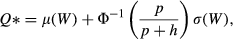
Consider the impact of expansion shocks on the ordering level. We expect the mean demand as well as the standard deviation of demand to increase with expansion shock. Thus, we expect retailers to order more and therefore carry more inventories when there is an expansion shock to the economy. Next, consider the impact of contraction shocks. When they experience a contraction shock, we expect retailers to forecast a lower mean demand but higher standard deviation of demand. Retailers are expected to reduce their ordering quantity when the decrease in mean demand is more than the increase in safety stock. On the other hand, retailers could increase their inventory investment during contraction shocks when the increase of safety stock is more than the decrease in inventory due to decline in mean demand. Thus, the impact of contraction shocks on ordering quantity, and inventory investment, would depend on whether the mean effect dominates or the safety stock effect dominates. Since the relative impact of a contraction shock on mean and standard deviation of demand is an empirical issue, we offer equivocal hypotheses for contraction shocks. Our hypotheses are as follows:

H1a: Inventory investments of retailers increase during expansion shocks.

H1b: Inventory investments of retailers decrease during contraction shocks.

H1b_ALT: Inventory investments of retailers increase during contraction shocks.

The previous hypotheses treat firms as homogenous entities and capture the average reaction to macroeconomic shocks. An important limitation of examining the average reaction of retailers is that it remains unclear whether retailers differ in their inventory investment behavior. More specifically, we wish to examine if retailers who are otherwise similar in all respects except stockout and holding costs have different inventory investment behavior. Such a difference would occur if these retailers differ in the extent to which they change their safety stock.

Consider two groups of retailers who differ based on their service levels, z ₁ > 0 and z ₂ > 0, but are similar in all other respects. As stated earlier, we expect macroeconomic shocks to affect both the mean and standard deviation of demand. For a given change in mean demand, we expect retailers in both groups to change their inventory investment by the same amount. However, the impact of standard deviation of demand on inventory investment would vary across retailers, since firms could differ in the amount by which they change their safety stock. The ordering quantity of the two retailers may be written as:

Retailers	Ordering quantity during expansion shocks	Ordering quantity during no shocks	Ordering quantity during contraction shocks
High service level	$Q_{1}^{E} = μ^{E} + z_{1} σ^{E}$	Q ₁ = μ + z ₁ σ	$Q_{1}^{C} = μ^{C} + z_{1} σ^{C}$
Low service level	$Q_{2}^{E} = μ^{E} + z_{2} σ^{E}$	Q ₂ = μ + z ₂ σ	$Q_{2}^{C} = μ^{C} + z_{2} σ^{C}$

where the superscripts E and C refer to expansion and contraction shocks, respectively. Below, we highlight the impact of expansion and contraction shocks on difference in ordering behavior across two retailers. The counterfactual comparison is with respect to the base‐case situation with no shock. We enumerate the differential impact for different signs of z ₁ and z ₂. Consistent with the assumptions in previous hypotheses we expect μ ^E > μ > μ ^C > 0 and σ ^E > σ > 0; σ ^C > σ > 0. In addition, since retailer 1 is a higher service level compared to retailer 2, we expect z ₁ > z ₂ > 0.

Consider the impact of expansion shocks on the ordering levels of the low and high service level retailers. We find that high service level retailers will order more and hence have a larger inventory investment compared to that of low service level retailers under all scenarios. On the other hand, there are three scenarios in the case of contraction shocks. In scenarios 1 and 2, we find that the inventory investment of low service level retailers will decrease more compared to high service level retailers. However, in scenario 3, we find that the inventory investment of all firms' increases during contraction shocks, as the increase in safety stock due to higher uncertainty dominates the decrease due to decline in mean demand. In this scenario, we find that inventory of high service level retailers increases by more compared to that of low service level retailers.

Impact of expansion shocks	Impact of contraction shocks
$Q_{1}^{E} - Q_{1} > Q_{2}^{E} - Q_{2} > 0$	Scenario 1: $Q_{2}^{C} - Q_{2} < Q_{1}^{C} - Q_{1} < 0$ if z ₂(σ ^C −σ) < z ₁(σ ^C −σ) < (μ−μ ^C); Scenario 2: $Q_{2}^{C} - Q_{2} < 0 < Q_{1}^{C} - Q_{1}$ if z ₂(σ ^C −σ) < (μ−μ ^C ) < z ₁ (σ ^C −σ); Scenario 3: $0 < Q_{2}^{C} - Q_{2} < Q_{1}^{C} - Q_{1}$ if (μ−μ ^C ) < z ₂ (σ ^C −σ) < z ₁ (σ ^C −σ).

Impact of expansion shocks

Impact of contraction shocks

Q_{1}^{E} - Q_{1} > Q_{2}^{E} - Q_{2} > 0

Scenario 1:

Q_{2}^{C} - Q_{2} < Q_{1}^{C} - Q_{1} < 0

if z ₂(σ ^C −σ) < z ₁(σ ^C −σ) < (μ−μ ^C);

Scenario 2:

Q_{2}^{C} - Q_{2} < 0 < Q_{1}^{C} - Q_{1}

if z ₂(σ ^C −σ) < (μ−μ ^C ) < z ₁ (σ ^C −σ);

Scenario 3:

0 < Q_{2}^{C} - Q_{2} < Q_{1}^{C} - Q_{1}

if (μ−μ ^C ) < z ₂ (σ ^C −σ) < z ₁ (σ ^C −σ).

The newsvendor model offers unambiguous predictions when there are expansion shocks:

H2a: Inventory investment of high service level retailers will increase by more compared to that of low service level retailers during expansion shocks.

On the other hand, the predictions of the newsvendor model vary based on the relative impact of contraction shocks on mean and standard deviation of demand:

H2b: Inventory investment of low service level retailers will decrease by more compared to that of high service level retailers during contraction shocks.

H2b_ALT: Inventory investment of high service level retailers will increase by more compared to that of low service level retailers during contraction shocks.

3. Research Methodology

The empirical tests of proposed hypotheses require us to capture variations in inventory investment across retailers (i.e., high service level vs. low services level) as well as across time variations (expansion vs. contraction shocks) for a given retailer. First, we discuss the methodology that we employ to measure macroeconomic shocks from the quarterly GDP reports. This methodology has been widely used in the macroeconomics literature. Second, we explain the autoregressive distributed lag model (ARDL) that permits the dynamic specification required to quantify the short‐term and long‐term impacts of macroeconomic shocks on inventory investment.

3.1. Measuring Economic Shocks

Economic shocks are generated from GDP time series using a two‐step process from Lamey et al. (2007, 2012). In the first step, we use a standard Hodrick‐Prescott (HP) filter to extract the cyclical component of GDP. Next, we generate measures of macroeconomic shocks from the cyclical component.

The observed GDP series is composed of a linear trend and cyclical variation around the trend: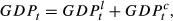

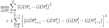
{GDP}_{t} = {GDP}_{t}^{l} + {GDP}_{t}^{c},

where

{GDP}_{t}^{l}

and

{GDP}_{t}^{c}

are trend and cyclical components of the observed GDP at time t. The HP filter (Hodrick and Prescott 1997) is used to decompose the GDP series into its two components. The HP filter extracts a cyclical component from the observed GDP series by solving the following minimization problem:

{SHOCK}_{t}^{Exp} = {GDP}_{t}^{c} - {GDP}_{Prior Trough}^{c},

where λ is the smoothing parameter. The objective is to minimize the first term in the above equation, subject to the second term in the equation. As λ → 0, the long‐term trend approximates the series, and as λ → ∞, all variation in the observed GDP series is attributed to cyclicality. The smoothing parameter is not estimable from data, but rather provided by the researcher. Extensive work in the macroeconomics literature suggests that, for quarterly data, λ = 1600 is most appropriate (see Hodrick and Prescott 1997, Ravn and Uhlig 2002). Since the evolution in a GDP series can be attributed to changes in inflation, consistent with previous research (see Lamey et al. 2007), we use constant dollars by chaining our GDP series to 1983 dollars and using the natural log of the series before applying the filter.

The positive cyclical component represents the expansion in the economy, whereas the negative values are indicative of contractions in the economy. Consistent with prior literature, we measure the magnitude of shocks in following way (see Cover 1992, Lamey et al. 2007, Thoma 1994):

{SHOCK}_{t}^{Exp} = {GDP}_{t}^{c} - {GDP}_{Prior Trough}^{c},

{SHOCK}_{t}^{Cont} = {GDP}_{Prior Peak}^{c} - {GDP}_{t}^{c},

where

{SHOCK}_{t}^{Exp}

and

{SHOCK}_{t}^{Cont}

are the expansion and contraction shocks.

{GDP}_{Prior Trough}^{c}

and

{GDP}_{Prior Peak}^{c}

are the values of

{GDP}^{c}

on prior trough and prior peak, respectively. Thus, with this operationalization,

{SHOCK}_{t}^{Cont}

and

{SHOCK}_{t}^{Exp}

take a positive value that makes it easy to interpret the coefficients.

3.2. Impact of Macroeconomic Shocks on Inventory Investment

We now explain the model used to study the impact of macroeconomic shocks on inventory investment. We consider two methodologies to test our hypotheses. First, we consider an ARDL to estimate the impact of macroeconomic shocks on inventory for the following reasons: (i) it is theoretically well motivated because it is derived from the adaptive expectations model of a manager's response to changes, (ii) it permits us to calculate the short‐ and long‐term impact of macroeconomic shocks on changes in inventory investment, and (iii) it is flexible enough to permit different lag lengths. The ARDL model was first proposed by Nerlove (1958) and has been used extensively since to study short‐ and long‐run impacts of product quality (Mitra and Golder 2006), real interest rates (Edison and Pauls 1993), leading output indicators (Clements and Galvao 2009), and many other variables of interest. The details of model derivation appear in Online Appendix A1.

Second, we consider a Vector Auto Regressive (VAR) model to test our hypotheses. VAR models are multivariate autoregressive models in which each endogenous variable is regressed against its own lagged values and those of other endogenous variables in the system. They have been used extensively in macroeconomics, finance, and marketing since the seminal work of Sims (1980). VAR models are appropriate for modeling long time series data with several endogenous variables. Another notable feature of this technique is that it allows policy simulations or intervention analysis using impulse response functions (IRF). An IRF is used for determining the impact of a unit shock to one endogenous variable on the rest of the system. Since VAR models are criticized for being atheoretical we use them as a robustness check.

3.2.1. Autoregressive Distributed Lag Formulation

Retail industries exhibit strong seasonal trends; therefore, a quarterly analysis of inventory investment should take into consideration seasonality that can explain significant variations in inventory investment across quarters. To account for this, we use change in log inventory between quarter t and t − 4 (ΔLINVT _it) as the measure of inventory investment. We use the symbol Δ to indicate fourth difference. In addition to accounting for quarterly seasonality, fourth differencing also has the following advantages. It enables us to eliminate the retailer‐fixed effect that would typically be included in the retailer‐level inventory investment model (Gaur et al. 2009, Gaur and Kesavan 2009, Rumyantsev and Netessine 2007). In addition, the fourth‐differenced variables can be interpreted as year‐over‐year change. They may be interpreted as the year‐on‐year change in the respective quarterly variable. Thus, the measure of inventory investment is the year‐on‐year growth in quarterly inventory.

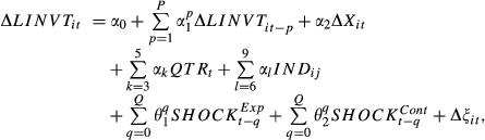
We use a general ARDL(p,q) model to test our hypotheses. Here, p is the number of lags of the dependent variable and q is the number of lags of the independent variable. We model inventory investment (ΔLINVT _it) as a function lagged inventory investment (ΔLINVT _it−p), changes in several contemporaneous control variables (ΔX _it), and contemporaneous and lagged effect(s) of shocks (

{SHOCK}_{t - q}^{Exp}

{SHOCK}_{t - q}^{Cont}

). Finally, we use fixed effects for industry segments at two‐digit SIC (IND _ij) and quarters (QTR _t) to capture any unobserved heterogeneity. We include the quarter dummies to be conservative and account for any residual seasonality effects that may not be captured by the fourth differencing. Our proposed model specification is

\begin{matrix} Δ {LINVT}_{it} & = α_{0} + \sum_{p = 1}^{P} α_{1}^{p} Δ {LINVT}_{it - p} + α_{2} Δ X_{it} \\ + \sum_{k = 3}^{5} α_{k} {QTR}_{t} + \sum_{l = 6}^{9} α_{l} {IND}_{ij} \\ + \sum_{q = 0}^{Q} θ_{1}^{q} {SHOCK}_{t - q}^{Exp} + \sum_{q = 0}^{Q} θ_{2}^{q} {SHOCK}_{t - q}^{Cont} + Δ ξ_{it}, \end{matrix}

where i, j, and t are notations for retailers, industry segment, and quarter, respectively. The above autoregressive formulation permits the impact of macroeconomic shocks on inventory investment to peak immediately or in up to the qth subsequent quarter and thereafter decline geometrically. The delay in impact of shock on inventory investment could be an artifact of lead time in supply chains. As no theory underlies when the shocks should peak, we test for multiple values of p and q to allow our data to determine the best values. While doing so, we also keep in mind that higher order values of q can be problematic, as it leads to greater multicollinearity. Consistent with previous research (see Kalaignanam et al. 2013), we test for lag length using Schwarz Bayesian Criterion (SBC = −2*LL + [Log(N)]*K), where LL is log likelihood, N is sample size, and K is the number of estimated parameters. Please note that in the above equation, inventory investment and other explanatory variables (X) are fourth differenced while the shock variables are differenced with respect to their previous peak or trough.⁵

3.2.2. Short and Long‐Term Impacts

This dynamic model specification permits us to capture the short‐ as well as long‐term impacts of shocks on inventory investment. An illustration of our econometric model specification is shown in Figure 1. For illustration purposes, we use the ARDL(1,1) specification. The inventory investment of retailer i at time t is impacted by a shock at time t and that from time t − 1. These impacts are measured by coefficients

θ_{1}^{0}

and

θ_{1}^{1}

, respectively. The sum of these two coefficients (

θ_{1}^{0} + θ_{1}^{1}

) is the short‐term effect (STE) of shocks. The shock from t − 2 impacts inventory investment at time t − 1, which in turn impacts inventory investment at time t through the coefficient α ₁. Similarly, the shock from t − 3 impacts inventory investment at time t − 2 through the coefficient α _1, and so on and so forth. Thus, the coefficient of the autoregressive term (also called as decay parameter) captures the impact of all shocks preceding t − 1. This impact is called the carryover impact of shocks. The sum total of short‐term effect and carryover effect is called long‐term effect (LTE) and is given by

(θ_{1}^{0} + θ_{1}^{1}) / (1 - α_{1})

. The larger the value of α _1, the more persistent the effects of macroeconomic shocks are on changes in inventory investment (i.e., impact of shocks on inventory investment decays slowly).

Figure 1

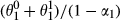
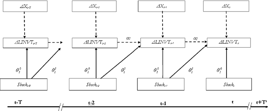
Illustration of Proposed Econometric Model SpecificationNote: For illustration purposes, expansion shock coefficients and ARDL(1,1) specification are exemplified

For the general ARDL(p,q) formulation, we calculate the STE and LTE of macroeconomic shocks on changes in inventory investment using the parameters

θ_{1}^{q}

and

θ_{2}^{q}

, and the decay parameter α ₁.

	Expansion	Contraction
STE	$(\sum_{q = 0}^{Q} θ_{1}^{q})$	$(\sum_{q = 0}^{Q} θ_{2}^{q})$
LTE	$\frac{(\sum_{q = 0}^{Q} θ_{1}^{q})}{(1 - α_{1})}$	$\frac{(\sum_{q = 0}^{Q} θ_{2}^{q})}{(1 - α_{1})}$

To test the statistical significance of the STE and LTE, we calculate the variance associated with them using Cramer's Theorem. The detailed expression for variance of these terms appears in Appendix A2.⁶

3.2.3. Controls

Consistent with our theorization and extant literature, we control for demand‐ and supply‐side factors that may impact inventory investment. The two demand‐side factors that influence inventory investment are changes in sales (measured as change in log sales, ΔLSALES _it) and changes in gross margin (measured as change in log gross margin, ΔLMRGN _it). On the supply side, the lead time of a retailer determines the rate at which the purchases made by a retailer show up in the books of a retailer, hence impacting the observed inventory investment. Consistent with Rumyantsev and Netessine (2007), we proxy for lead time using days payable (measured as change in log days payable, ΔLDP _it). In addition, we control for impact of new store openings or existing store closings on changes in inventory investment by including changes in assets held by retailers (measured as change on log assets, ΔLAT _it). These control variables replace the ΔX in Equation 5:

\begin{matrix} Δ {LINVT}_{it} & = α_{0} + \sum_{p = 1}^{P} α_{1}^{p} Δ {LINVT}_{it - p} + α_{2} Δ {LMRGN}_{it} \\ + α_{3} Δ {LSALES}_{it} + α_{4} Δ {LDP}_{it} + α_{5} Δ {LAT}_{it} \\ + \sum_{k = 6}^{8} α_{k} {QTR}_{t} + \sum_{k = 9}^{12} α_{k} {IND}_{ij} \\ + \sum_{q = 0}^{Q} θ_{1}^{q} {SHOCK}_{t - q}^{Exp} + \sum_{q = 0}^{Q} θ_{2}^{q} {SHOCK}_{t - q}^{Cont} + Δ ξ_{it} . \end{matrix}

3.3. Estimation

There are five issues related to estimating Equation 6. First, to test the impact of service level on the relationship between macroeconomic shocks and changes in inventory investment, we test Equation 6 separately on a subsample of retailers' high and low ratios of stockout to inventory holding costs. The subsample analysis is a more conservative approach to testing moderating impact, as it reduces the sample size. In addition, this approach avoids interaction effects that can create severe multicollinearity, thereby leading to inflated standard errors and incorrect interpretation of the coefficients. We discuss the measurement of these variables and classification of firms in high and low groups in the next section.

Second, the contemporaneous shock terms (

{SHOCK}_{t}^{Exp}, {SHOCK}_{t}^{Cont}

) simultaneously impact the dependent variable (ΔLINVT _it) as well as the contemporaneous terms (ΔLMRGN _it , ΔLSALES _it, ΔLDP _it , ΔLAT _it), thereby biasing our coefficient estimates. For example, firms could have higher demand during expansion shocks resulting in higher margins, sales, and inventory. We handle this simultaneity using lagged values of change in margin (ΔLMRGN _it−q−1, ΔLMRGN _it−q−2), lagged values of change in sales (ΔLSALES _it−q−1, ΔLSALES _it−q−2), lagged values of change in days payable (ΔLDP _it−q−1, ΔLDP _it−q−2), and lagged values of change in assets (ΔLAT _it−q−1, ΔLAT _it−q−2) as our instruments. Our instruments predate the last included macroeconomic shocks by at least one quarter.

Third, the lagged dependent variable (ΔLINVT _it−p) can be influenced by the lagged value of macroeconomic shocks (

{SHOCK}_{t - q}^{Exp}, {SHOCK}_{t - q}^{Cont}

), thereby biasing our estimate of the long‐term impact of economic shocks. Therefore, we instrument it using the lagged value of the dependent variable predating the last shock included in the model by at least one quarter (ΔLINVT _it−q−1 , ΔLINVT _it−q−2).

Fourth, use of lagged dependent variables on the right‐hand side typically results in dynamic panel data bias. We argue that such a bias is not an issue in our case, as fourth differencing should remove any correlation between ΔLINVT _it−1 and Δξ _it. This is because the error in ΔLINVT _it (Δξ _it = ξ _it−ξ _it−4) and the error in ΔLINVT _it−1 (Δξ _it−1 = ξ _it−1−ξ _it−5) have no common error terms, and the errors are not autocorrelated. In addition, please note that ΔLINVT _it−1 is instrumented using previous lagged values, thus further reducing any residual autocorrelation.

Fifth, we estimate Equation 6 separately for expansion and contraction shock periods. This is required because the shock values are exclusive (i.e., only one type of shock exists at a given point of time); including both shocks in the same equation would render estimation impossible.

4. Data

The data for our empirical testing are obtained from COMPUTSTAT, which maintains a database of quarterly SEC filings of publicly traded retailers. The quarterly data for retailer‐level variables are obtained from COMPUSTAT. We extract 25 years of quarterly data (1985–2009) for all publicly traded retailers in two‐digit SIC 52–59, corresponding to retail sector. These SIC codes cover the following segments within retail: construction and home improvement (SIC = 52), department stores (SIC = 53), groceries and produce (SIC = 54), automobile dealers (SIC = 55), clothing and accessories (SIC = 56), furniture and white goods (SIC = 57), restaurants and eating outlets (SIC = 58), and others (drug stores, direct retailers, bookstores, stationery stores, florists, optical stores, news vendors, etc.) (SIC = 59). We obtain data on Consumer Price Index (CPI), used for adjusting variables in our analyses, to constant dollars from the Bureau of Economic Analysis (BEA). We use the 2005 value of the CPI as a base to adjust the variables. Thus, values of variables prior to 2005 are inflated while those observed after 2005 are deflated. Similarly, we obtain the quarterly GDP series of the United States from 1947 to 2009 from the BEA.

4.1. Data Merging and Cleanup

First, we apply the HP filter on the transformed (CPI adjusted and logged) quarterly GDP series (from 1947 to 2009) to detrend the series and extract the cyclical component. Second, we generate macroeconomic shocks from the cyclical component of GDP for merging with the remainder of the retailer‐level data. Since the quarterly GDP reports follow calendar time (Q1 = Jan to Mar, Q2 = Apr to Jun, Q3 = Jul to Sep, and Q4 = Oct to Dec), we retain retailers which have fiscal years ending in either December or January.⁷ We found that January was the second most popular month (after December) to have the fiscal year end in the retail industry. About 38% of the firms had their fiscal year end in January. To avoid discarding such a large amount of data, we decided to include the retailers having January fiscal year ends along with those having December fiscal year ends. We align the macroeconomic shock from January to March with the first quarter data for retailers with fiscal year ends in January. In addition, consistent with Kesavan et al. (2010), we drop SIC 58 (restaurants and eating outlets) and 55 (automobile dealers) from our analyses because retailers in these industries have a significant service component, and, consequently, inventory management behavior is only partly related to macroeconomic shocks. In addition, we drop SIC 54 (groceries and produce) from our analyses as this segment is acyclical to economic shocks.⁸ We trim the top 1% and bottom 1% of observations based on the dependent variable. This approach ensures that our analyses are not unduly influenced by extreme outliers. Our final sample thus consists of over 360 retailers and about 10,000 retailer quarter observations.

4.2. Measurement

4.2.1. Inventory Investment

The dependent variable, inventory investment, is measured as ΔLINVT _it = LINVT _it −LINVT _it−4, where LINVT is Log (INVT _it). Thus, inventory investment measures year‐over‐year change in inventory between the same quarter. The details of operationalization of other variables and their data sources are summarized in Table 1.

Table 1
Variables and Data Sources

Variable Measure Data source

CPI Consumer price index as measure of inflation Bureau of economic analysis (BEA)

Gross domestic product (GDP _t) Log (CPI adjusted GDP) BEA

INVT CPI adjusted inventory (INVTQ) COMPUSTAT

COGS CPI adjusted cost of goods sold (COGSQ) COMPUSTAT

REVT CPI adjusted revenues (REVTQ) COMPUSTAT

AP CPI adjusted accounts payable (APQ) COMPUSTAT

ACT CPI adjusted current assets (ACTQ) COMPUSTAT

LCT CPI adjusted current liabilities (LCTQ) COMPUSTAT

AT CPI adjusted total assets (ATQ) COMPUSTAT

INT CPI adjusted interest paid (XINTQ) COMPUSTAT

LTD CPI adjusted long‐term debt (DLTTQ) COMPUSTAT

SHO Number of shares outstanding (CHSOQ) COMPUSTAT

SHPRC Closing share price at end of quarter (PRCCQ) COMPUSTAT

NI Net income in quarter (NIQ) COMPUSTAT

Log inventories—LINVT _it Log(INVT _it)

Log sales—LCOGS _it Log (COGS _it)

Log assets—LAT_it Log (AT_it )

Gross margin—MRGN _it (REVT _it −COGS _it)/REVT _it)

Log gross margin—LMRGN _it Log (MRGN _it)

Days payable (Lead time)—DP _it 365/(4**COGS* _it/AP _it)

Log days payable—LDP _it Log (DP _it)

Change in inventory investment—ΔLINVT _it LINVT _it −LINVT _it−4

Change in log sales—ΔLSALES _it LCOGS _it −LCOGS _it−4

Change in log gross margin—ΔLMRGN_it LMRGN _it −LMRGN _it−4

Change in log lead time—ΔLDP _it LDP _it −LDP _it−4

Change in log asset—ΔLAT _it LAT _it −LAT _it−4

Debt cost t—DC _it INT _it /(LCT _it + LTD _it)

Equity cost—EC _it NI _it /(SHO _it * SHPRC _it)

Weighted average cost of capital—WACC _it Weighted average of (DC _it + EC _it)

Stockout to inventory holding cost ratio—SCIC _it SCIC _it = 1 if MRGN _it−q−t' /WACC _it−q−1 > 50th percentile within given two‐digit SIC classification, else SCIC _it = 0

Variable	Measure	Data source
CPI	Consumer price index as measure of inflation	Bureau of economic analysis (BEA)
Gross domestic product (GDP _t)	Log (CPI adjusted GDP)	BEA
INVT	CPI adjusted inventory (INVTQ)	COMPUSTAT
COGS	CPI adjusted cost of goods sold (COGSQ)	COMPUSTAT
REVT	CPI adjusted revenues (REVTQ)	COMPUSTAT
AP	CPI adjusted accounts payable (APQ)	COMPUSTAT
ACT	CPI adjusted current assets (ACTQ)	COMPUSTAT
LCT	CPI adjusted current liabilities (LCTQ)	COMPUSTAT
AT	CPI adjusted total assets (ATQ)	COMPUSTAT
INT	CPI adjusted interest paid (XINTQ)	COMPUSTAT
LTD	CPI adjusted long‐term debt (DLTTQ)	COMPUSTAT
SHO	Number of shares outstanding (CHSOQ)	COMPUSTAT
SHPRC	Closing share price at end of quarter (PRCCQ)	COMPUSTAT
NI	Net income in quarter (NIQ)	COMPUSTAT
Log inventories—LINVT _it	Log(INVT _it)
Log sales—LCOGS _it	Log (COGS _it)
Log assets—LAT_it	Log (AT_it )
Gross margin—MRGN _it	(REVT _it −COGS _it)/REVT _it)
Log gross margin—LMRGN _it	Log (MRGN _it)
Days payable (Lead time)—DP _it	365/(4*COGS _it/AP _it)
Log days payable—LDP _it	Log (DP _it)
Change in inventory investment—ΔLINVT _it	LINVT _it −LINVT _it−4
Change in log sales—ΔLSALES _it	LCOGS _it −LCOGS _it−4
Change in log gross margin—ΔLMRGN_it	LMRGN _it −LMRGN _it−4
Change in log lead time—ΔLDP _it	LDP _it −LDP _it−4
Change in log asset—ΔLAT _it	LAT _it −LAT _it−4
Debt cost t—DC _it	INT _it /(LCT _it + LTD _it)
Equity cost—EC _it	NI _it /(SHO _it * SHPRC _it)
Weighted average cost of capital—WACC _it	Weighted average of (DC _it + EC _it)
Stockout to inventory holding cost ratio—SCIC _it	SCIC _it = 1 if MRGN _it−q−t' /WACC _it−q−1 > 50th percentile within given two‐digit SIC classification, else SCIC _it = 0

4.2.2. Service Level

The service level of a retailer is determined by the ratio of stockout to inventory holding cost incurred by the retailer. The stockout cost, or the opportunity cost of lost sales, at the firm level is unobservable to an econometrician. We follow the firm‐level inventory literature to use gross margin as a proxy for stockout cost, as it captures the markup that retailers obtain on the merchandise they sell. Therefore, the larger the gross margin, the higher the opportunity cost of lost sales. We follow Irvine (1981), Raman and Kim (2002), Rumyantsev and Netessine (2007), and Rajagopalan (2012) and use weighted average cost of capital (WACC) as our measure of inventory holding cost. WACC is measured as weighted average of cost of debt incurred and cost of equity earned by a retailer. The weights are the relative proportion of debt and equity. The debt cost is measured as interest paid on outstanding short‐ and long‐term debt. The equity cost is measured as quarterly return generated on the outstanding market value of the retailer. We obtain these data from COMPUSTAT. Consistent with our theorization, we calculate the stockout to inventory holding cost ratio for classifying retailers into different types of service levels. We use median split to classify a retailer into a high or low group if the retailer falls in the top 50th or bottom 50th percentile in the quarter predating the last macroeconomic shock included in the model. Using the median split ensures the most conservative test of our hypotheses.

4.2.3. Sensitivity of Measurement

There are a few issues pertaining to measurement of service level. First, we address unobservable heterogeneity that might confound our analysis. A key assumption underlying our approach is that high and low service level retailers face similar demand shocks. We check the plausibility of this assumption by estimating a demand model in which we capture the impact of macroeconomic shocks. The model specification is similar to that reported in Equation 5. We use changes in gross margin, changes in selling general and administrative expenses, and changes in assets as controls. The results of the demand model are reported in Appendix 3 (see Table A3‐1). The results suggest that during expansion (contraction) shocks the demand for both types of retailers increases (decreases). However, the impact of these macroeconomic shocks on the demand faced by the two types of retailers is similar. Thus, our service level measure is not sensitive to the demand characteristics of these retailers.

Second, prior research (see Anderson et al. 2006) shows that there are direct and indirect components to this opportunity cost. The direct component refers to loss of profit due to the focal item not being sold, which otherwise would have sold had it been available. The indirect cost refers to loss of profit on complementary products and losses arising due to a lower probability of future orders. Since our measurement of stockout cost is at an aggregate level, our measure only proxies for the direct costs. We acknowledge that indirect opportunity costs cannot be captured using an aggregate approach. However, since both types of retailers likely cater to different customer segments, the customers of high service level retailers are likely to be more sensitive to service quality compared to those of low service level retailers. Thus, high service level retailers are also likely to face higher indirect opportunity costs. This artifact suggests that our measurement of stockout costs is conservative. However, we acknowledge that this assumption is not testable using public data.

Lastly, inventory holding cost is driven by the physical cost of holding inventory as well the opportunity cost of capital. Our measure of inventory holding cost, WACC, serves as a proxy for opportunity cost but does not capture the physical cost of holding inventory. While ignoring the physical cost of holding inventory may be justified if it is small relative to the opportunity cost of capital, it remains unclear if this is the case and whether our results are impacted by this limitation of WACC.

4.3. Data Summary

We summarize our data in Table 2. Across the 100 quarters of data, we find on average the quarterly COGS in our sample is $226 m and inventory holding is also $226 m. An average retailer in our sample has assets to the tune of $688 m. The data also suggest that, on average, during expansion (contraction) the GDP increased (decreased) by 0.83% (0.95%) compared to the previous trough (peak). Importantly, the average gross margin, proxy for stockout costs, is 57% of sales. Conversely, the mean WACC (proxy for inventory holding cost) is 1.6% of the capital. The mean SCIC ratio is 98. When comparing the mean values across the high and low service level groups, we find that high service level retailers have a higher gross margin (i.e., stockout costs) and lower WACC (i.e., inventory holding costs) compared to the low service level retailers. The mean values on each control variable are similar across the groups, thereby suggesting that there are no systematic differences, except on service levels.

Table 2
Summary Statistics

Variable Overall High service level Low service level

Mean SD Mean SD Mean SD

INVT ($) 226.124 484.846 226.444 455.238 225.661 524.814

MRGN (%) 57.140 12.002 60.289 9.897 52.580 13.255

WACC (%) 1.581 1.823 0.762 0.399 2.460 2.286

SCIC 97.784 576.249 168.809 926.677 26.723 110.532

SHOCK ^EXP (%) 0.829 0.544

SHOCK ^CONT (%) 0.949 1.170

COGS ($) 226.235 531.640 220.785 514.101 234.129 556.012

AT ($) 688.555 1513.651 690.046 1456.923 686.394 1592.357

Days payable (DP) 79.830 51.492 88.707 52.155 66.965 47.671

Variable	Overall	High service level	Low service level
INVT ($)	226.124	484.846	226.444	455.238	225.661	524.814
MRGN (%)	57.140	12.002	60.289	9.897	52.580	13.255
WACC (%)	1.581	1.823	0.762	0.399	2.460	2.286
SCIC	97.784	576.249	168.809	926.677	26.723	110.532
SHOCK ^EXP (%)	0.829	0.544
SHOCK ^CONT (%)	0.949	1.170
COGS ($)	226.235	531.640	220.785	514.101	234.129	556.012
AT ($)	688.555	1513.651	690.046	1456.923	686.394	1592.357
Days payable (DP)	79.830	51.492	88.707	52.155	66.965	47.671

5. Results

In this section, we discuss the results of our analyses. First, we explain our model selection results by comparing the results of models with different lag length specifications. Second, we discuss our results of testing Hypotheses 1a and 1b. Third, we discuss the moderating impact of stockout to inventory holding cost (i.e., “service levels”) and discuss results for Hypotheses 2a and 2b. Finally, we discuss several robustness checks of our results.

5.1. Model Selection

In Table 3, we report the model fit statistics of different model specifications. We start with the simplest model with no autoregressive terms and no distributed lags of the macroeconomic shocks, ARDL(0,0). We subsequently add lags and autoregressive terms in the model. We report fit statistics separately for expansion and contraction periods. The comparative model fit statistics suggest that the Schwarz Bayesian Criterion is lowest for ARDL(1,1) specification both during expansion and contraction shocks. Thus, we use ARDL(1,1) specification for testing our hypotheses. This one lag of macroeconomic shock variable suggests that the impact of these shocks on changes in inventory investment can peak one quarter after the shock hits the retailer. We discuss the robustness of our results to alternate model specification in section 5.5.

Table 3
Results: Model Comparison

Schwartz's Bayesian Criterion Expansion Contraction

ARDL(0,0) −4925.49 −5540.67

ARDL(0,1) −5482.72 −5825.7

ARDL(0,2) −5510.23 −5697.9

ARDL(1,0) −7368.91 −7438.43

ARDL(1,1)* −7372.46* −7442.26*

ARDL(1,2) −7241.05 −7373.05

ARDL(2,0) −7270.06 −7405.94

ARDL(2,1) −7267.07 −7402.19

ARDL(2,2) −7264.51 −7399.24

Schwartz's Bayesian Criterion	Expansion	Contraction
ARDL(0,0)	−4925.49	−5540.67
ARDL(0,1)	−5482.72	−5825.7
ARDL(0,2)	−5510.23	−5697.9
ARDL(1,0)	−7368.91	−7438.43
ARDL(1,1)*	−7372.46*	−7442.26*
ARDL(1,2)	−7241.05	−7373.05
ARDL(2,0)	−7270.06	−7405.94
ARDL(2,1)	−7267.07	−7402.19
ARDL(2,2)	−7264.51	−7399.24

Note: ARDL (p,q), p (q) number of lags of dependent (shock) variable. * Selected model specification with lowest SBC.

5.2. Inventory Investment Hypotheses

Consider the results of testing Hypotheses 1a and 1b using the ARDL(1,1) model as shown in Table 4. As the independent and dependent variables in the model are logged so the coefficients can be interpreted as elasticities, we find that a 1% increase in expansion (contraction) shock is associated with an increase (decrease) in inventory investment by 1.867%, p < 0.01 (1.075%, p < 0.05). This 1% increase in expansion (contraction) shock corresponds to a 1% increase (decrease) in the GDP compared to the previous trough (peak) (Lamey et al. 2007). We note that the effects of shocks on inventory growth are much larger than that of sales growth. A 1% increase in sales growth is associated with 0.474%, p < 0.01 (0.405%, p < 0.01) increase in inventory growth during expansion (contraction) periods. These results suggest that the change in inventory investment in response to changes in future demand, as implied by economic shock, is much larger than the change due to current period sales.

Table 4
Results: Impact of Macro‐economic Shocks on Inventory Investment

Dependent variable—ΔLINVT _it Expansion Contraction

Coeff. SE Coeff. SE

ΔLINVT _it−1 * 0.419 0.026 0.458 0.022

ΔLMRGN _it * 0.346 0.082 0.176 0.055

ΔLSALES _it * 0.474 0.059 0.405 0.043

ΔLDP _it * 0.054 0.027 0.150 0.022

ΔLAT _it * 0.105 0.039 0.121 0.029

${SHOCK}_{t}^{Exp}$ 1.867 0.699

${SHOCK}_{t - 1}^{Exp}$
−0.917 0.677

${SHOCK}_{t}^{Cont}$
−1.075 0.572

${SHOCK}_{t - 1}^{Cont}$
0.305 0.680

Intercept −0.043 0.019 −0.015 0.007

Quarter effects Three significant One significant

Industry segment effects None significant One significant

H1a H1b

Short‐term effects 0.950 0.347 −0.770 0.250

Long‐term effects 1.636 0.597 −1.420 0.458

Sample size N (No. of retailers) 4357 (355) 5059 (360)

R ² total 0.638 0.675

Dependent variable—ΔLINVT _it	Expansion	Contraction
ΔLINVT _it−1 *	0.419	0.026	0.458	0.022
ΔLMRGN _it *	0.346	0.082	0.176	0.055
ΔLSALES _it *	0.474	0.059	0.405	0.043
ΔLDP _it *	0.054	0.027	0.150	0.022
ΔLAT _it *	0.105	0.039	0.121	0.029
${SHOCK}_{t}^{Exp}$	1.867	0.699
${SHOCK}_{t - 1}^{Exp}$	−0.917	0.677
${SHOCK}_{t}^{Cont}$			−1.075	0.572
${SHOCK}_{t - 1}^{Cont}$			0.305	0.680
Intercept	−0.043	0.019	−0.015	0.007
Quarter effects	Three significant	One significant
Industry segment effects	None significant	One significant
	H1a	H1b
Short‐term effects	0.950	0.347	−0.770	0.250
Long‐term effects	1.636	0.597	−1.420	0.458
Sample size N (No. of retailers)	4357 (355)	5059 (360)
R ² total	0.638	0.675

Note: All italicized coefficients have p < 0.05. *Variable has been instrumented using lags from t − 2 and t − 3.

We may also compute the short‐term and long‐term effects of these shocks on inventory growth. In the short term, we find that a 1% increase in expansion (contraction) shock in the current quarter is associated with an increase (decrease) in inventory investment by 0.950%, p < 0.01 (0.770%, p < 0.01) in the current and subsequent quarter. As far as the total effect is concerned, we find that a 1% increase in expansion (contraction) shock leads to a 1.636%, p < 0.01 (1.420%, p < 0.01) increase (decrease) in inventory investment. We find that 58% of total impact is realized in the first two quarters. The impact peaks in the quarter after the shock occurs and thereafter declines at a geometric rate. Since the decay parameters for both expansion and contraction shocks are similar (0.419 and 0.458), we find that 90% of both types of shocks are dissipated in about three quarters. Thus, in support of H1a and H1b, we find that inventory investment moves pro‐cyclical to macroeconomic shocks.

The model is well specified as evident from significance and directionality of control variables. Consistent with prior literature (Gaur et al. 2005a,b, Gaur and Kesavan 2009, Rumyantsev and Netessine 2007, Kesavan et al. 2010), we find that sales growth, gross margin, lead time, and assets are positively related to inventory investment.

5.3. Stockout and Inventory Holding Cost Hypotheses

In our theorization and conceptual development, we hypothesized that service levels of retailers will drive inventory investment decisions during macroeconomic shocks. We estimate our proposed model specification on different subsamples of retailers with high and low ratios of stockout to inventory holding costs. Consider the reaction of high service level retailers to expansion shocks. The estimation results are presented in Table 5. A 1% increase in GDP compared to the previous trough is associated with a 2.342% (p < 0.01) increase in inventory growth in the current quarter and 1.700% (p < 0.01) in the short term (current quarter + next quarter). A 1% increase in sales growth is associated with only A 0.537% (p < 0.01) increase in inventory growth. Comparing the reaction of retailers to expansion shock and sales, we conclude that retailers with high service levels appear to aggressively increase their inventory in anticipation of future demand. The long‐term effect of the expansion shock is much larger (3.104%, p < 0.01), as expected.

Table 5
Results: Service Level

Dependent variable—ΔLINVT _it High (SCIC = 1) Low (SCIC = 0)

Expansion Contraction Expansion Contraction

Coeff. SE Coeff. SE Coeff. SE Coeff. SE

ΔLINVT _it−1 ¹ 0.452 0.045 0.413 0.028 0.475 0.029 0.435 0.042

ΔLMRGN _it ¹ 0.366 0.100 0.178 0.081 0.139 0.076 0.207 0.076

ΔLSALES _it ¹ 0.537 0.096 0.480 0.059 0.446 0.063 0.406 0.074

ΔLDP _it ¹ 0.096 0.045 0.194 0.028 0.049 0.031 0.114 0.035

ΔLAT _it ¹ −0.093 0.066 0.143 0.037 0.126 0.047 0.102 0.053

${SHOCK}_{t}^{Exp}$ 2.342 1.141 1.455 0.955

${SHOCK}_{t - 1}^{Exp}$
−0.642 1.105 −0.855 0.917

${SHOCK}_{t}^{Cont}$
−0.353 0.792 −1.344 0.779

${SHOCK}_{t - 1}^{Cont}$
−0.101 0.934 0.069 0.930

Intercept −0.060 0.025 −0.007 0.017 −0.027 0.014 −0.024 0.014

Quarter effects One significant One significant One significant None significant

Industry segment effects None significant None significant None significant None significant

Short‐term effects 1.700 0.548 −0.454 0.346 0.601 0.469 −1.275 0.346

Long‐term effects 3.104 0.953 −0.774 0.565 1.144 0.859 −2.256 0.605

Sample size N (No. of retailers) 1969 (295) 2756 (300) 2365 (303) 2276 (305)

R ² total 0.538 0.678 0.679 0.674

H2a Expansion H2b Contraction

Diff SE Diff SE

Short‐term effects (high−low) 1.099 0.507 0.821 0.346

Long‐term effects (high−low) 1.960 0.904 1.482 0.587

Dependent variable—ΔLINVT _it	High (SCIC = 1)	Low (SCIC = 0)
ΔLINVT _it−1 ¹	0.452	0.045	0.413	0.028	0.475	0.029	0.435	0.042
ΔLMRGN _it ¹	0.366	0.100	0.178	0.081	0.139	0.076	0.207	0.076
ΔLSALES _it ¹	0.537	0.096	0.480	0.059	0.446	0.063	0.406	0.074
ΔLDP _it ¹	0.096	0.045	0.194	0.028	0.049	0.031	0.114	0.035
ΔLAT _it ¹	−0.093	0.066	0.143	0.037	0.126	0.047	0.102	0.053
${SHOCK}_{t}^{Exp}$	2.342	1.141			1.455	0.955
${SHOCK}_{t - 1}^{Exp}$	−0.642	1.105			−0.855	0.917
${SHOCK}_{t}^{Cont}$			−0.353	0.792			−1.344	0.779
${SHOCK}_{t - 1}^{Cont}$			−0.101	0.934			0.069	0.930
Intercept	−0.060	0.025	−0.007	0.017	−0.027	0.014	−0.024	0.014
Quarter effects	One significant	One significant	One significant	None significant
Industry segment effects	None significant	None significant	None significant	None significant
Short‐term effects	1.700	0.548	−0.454	0.346	0.601	0.469	−1.275	0.346
Long‐term effects	3.104	0.953	−0.774	0.565	1.144	0.859	−2.256	0.605
Sample size N (No. of retailers)	1969 (295)	2756 (300)	2365 (303)	2276 (305)
R ² total	0.538		0.678		0.679		0.674

	H2a Expansion	H2b Contraction
Short‐term effects (high−low)	1.099	0.507	0.821	0.346
Long‐term effects (high−low)	1.960	0.904	1.482	0.587

Note

All italicized coefficients have p < 0.05.

Variable has been instrumented using lags from t − 2 and t − 3.

The reaction of retailers with low service levels to expansion shock in the short term is 0.601 (p > 0.10) and in the long term is 1.144 (p > 0.10). Thus, in the short term, we find that high service level retailers (1.700, p < 0.01) increase their inventory investment by more compared to low service levels retailers (0.601, p > 0.10). The difference between the two is statistically significant (Difference = 1.009, p < 0.05), supporting H2a. Our conclusions remain unchanged even when we compare the long‐term reactions of these two types of retailers.

Next, consider the reaction of these two types of retailers to contraction shocks. We find that low service level retailers react aggressively to contraction shocks by decreasing their inventory investment. In the short term, a 1% increase in contraction shock is associated with a 1.275% (p < 0.01) decrease in inventory growth. The magnitude of this reaction is significantly more (Difference = 0.821, p < 0.01) compared to that of high service level retailers. Thus, we find statistical support for hypothesis H2b. Our conclusion holds even when we compare the long‐term effects.

In summary, our results indicate that there is a significant difference in inventory investment behavior between retailers with high and low ratios of stockout to holding costs. The observed differences in behavior between the two types of retailers appear rational based on the profit maximizing motive of the newsvendor model. These results have important implications for benchmarking inventory performance. Prior firm‐level inventory models consider factors such as sales growth and change in gross margin in determining the expected inventory level for retailers when benchmarking inventory performance and ignore economic shocks. In the next section, we investigate the implications of including economic shocks and service levels in these benchmarking models.

5.4. Robustness Checks

We perform several robustness checks to enhance confidence in our empirical analyses. We examine the robustness of our results to assumptions about exogeneity of macroeconomic shocks and service levels, to alternate model specifications, alternate measures of shock, alternate operationalization of high vs. low groups, and alternate estimation technique. To conserve space the detailed results of robustness analyses are reported in Appendix A4.

First, we perform Durbin‐Wu‐Hausman augmented regression to test for exogeneity of macroeconomic shocks (see Davidson and MacKinnon 1993). First, we regress macroeconomic shocks (expansion and contraction separately) on their lags from t − 2 to t − 5. These are appropriate instruments because they predate the included shocks by at least one quarter and they do not meet the temporal ordering condition for the decisions made by retailer at time t. Second, we include the residuals from the first stage (current and one lag) in our Equation 6. If the coefficients for residuals are statistically significant one cannot rule out endogeneity of the shock terms. The results suggest that coefficients for residual current and lag term of expansion shock and lag term for contraction shock are not significant. Thus, our assumption that both types of macroeconomic shocks are exogenous to the system is not violated. Most importantly, at an aggregate level the inventory investment across all industries can drive business cycle fluctuations; it is very unlikely that inventory investment decisions made by one retailer has the potential to impact the cyclicality in the economy. In other words, for a retail manager making inventory management decisions, the state of the economy is exogenously determined. No one retailer's inventory investment decision can bring about expansion and contractions in a large capitalistic economy such as the United States.

Second, while we use lagged values of ratio of stockout to holding costs for classifying retailers into high and low groups, we formally test if the relative position of a retailer changes between these groups as a result of macroeconomic shocks. We test this assumption by modeling the impact of expansion and contraction shocks on probability of a firm belonging in high group vis‐à‐vis the low group. We use random effects panel data probit model to estimate group membership of the key dependent variable: SCIC _it. We include the lagged value of the dependent variable (SCIC _it−1) as a control for state dependence. The impacts of expansion and contraction shocks on probability of a firm belonging in the high group vis‐à‐vis the low group is not statistically significant. The test establishes that the relative position of a firm in two groups remains unaffected by the macroeconomic shocks.

Third, we test the sensitivity of our results to several alternate model specifications. Recall that we developed a general ARDL model and chose the ARDL(1,1) specification based on model fit. We estimate a simple model with no autoregressive term and no distributed lag term [ARDL(0,0)]. The results suggest that directionality and significance of coefficients of shock terms as well as control variables are consistent with the results reported in Table 4. We subsequently add one distributed lag term making it a ARDL(0,1) specification. This is closest to our proposed specification, except for lack of an autoregressive term. Again, the significance and directionality of coefficients of shock terms suggest that adding an autoregressive term to the model does not influence our substantive conclusions.⁹ In our results, we find that 99% of impact of shocks is dissipated in about five quarters, and we report results of model with no autoregressive term but four distributed lag terms. Again, the total effect of expansion and contraction shocks is similar in directionality and significance.¹⁰

Fourth, while we use a conservative median split on service levels for classifying retailers into high and low groups, we test the sensitivity of these findings to alternate operationalizations of high and low groups. Alternatively, we classify retailers in high and low groups if they fall in the top 66th and bottom 33rd percentile, respectively. As expected, the results of this analysis are stronger than those reported in Table 4.

Fifth, since we fourth difference our dependent and independent variables, to be consistent with this operationalization we measure macroeconomic shock as fourth difference of cyclical component of GDP (

{SHOCK}_{t} = {GDP}_{t}^{c} - {GDP}_{t - 4}^{c}

). With this operationalization, positive (negative) values of shock indicate unexpected increases (decreases) in GDP. The findings from this analysis are consistent with those reported on Table 4. Thus, our results are not sensitive to operationalization of shocks.

Sixth, we use the quarterly Personal Consumption Expenditure (PCE) series instead of GDP to measure macroeconomic shocks. We find that PCE accounted for 62.5% of the GDP in 1970 and this percentage increased to 70% by 2009. We obtain similar results when we also measure macroeconomic shocks with the PCE series. This result provides additional support to our finding that macroeconomic shocks impact consumer spending and thus retailers' demand forecast and inventory management decisions.

Seventh, it can be argued that the numbers used in our GDP series are not released until a few days after the end of the quarter, and therefore the GDP series used by us may not be forward looking. Thus, we need to test the robustness of our findings to alternate measures of macroeconomic series which captures the forward‐looking behavior of consumers. We use the Consumer Confidence Index (CCI) reported by the Conference Board as an alternate measure of the state of the economy. CCI is measured through an extensive survey of consumer perceptions about the current state of the economy and their anticipated consumption behavior in the near future. While GDP has a clear linear trend and a high‐frequency cyclical component around it, the CCI series is essentially cyclical in nature.¹¹ Thus, changes in CCI are akin to unexpected changes in the cyclical component of GDP (see the above analysis). We operationalize macroeconomic shock as fourth difference change in CCI (SHOCK _t = CCI _t −CCI _t−4). With this operationalization positive (negative) values of shock indicate an increase (decrease) in consumer confidence. The results of this analysis are consistent with those reported in Table 4. This suggests that the quarterly GDP series maps consistently well with forward‐looking measures of consumer confidence.

Lastly, since we pass the entire quarterly GDP series time (1947 to 2009) through the HP filter to derive the cyclical component of GDP, it is plausible that the cyclical component of GDP at time t (where t < 2009) draws upon GDP information from future time periods. This artifact may influence the precision with which we are able to decompose the GDP series. Since our measure of shock captures the non‐anticipatory component, we generate an alternate shock measure which is truly non‐anticipatory in nature and does not rely on the availability of future GDP information. We generate 100 quarterly GDP time series, each containing one additional quarter of GDP information from 1985 to 2009. We pass each of these 100 time series through the HP filter and retain the cyclical component of the last quarter of the series. For example for 1985Q1 we pass the GDP series from 1947Q1 to 1985Q1 through the HP filter and retain the cyclical component of last quarter (1985Q1 in this case). We repeat this exercise 100 times and keep adding an additional quarter to the data. We use these cyclical components to generate expansion and contraction shock variables. We use this alternate shock variable to test out hypotheses. We find support for our proposed hypotheses. This suggests that while we use an entire GDP series to extract cyclical component, the shock measures to a large extent is non‐anticipatory in nature.

6. VAR Analysis of Economic Shocks

In this section, we perform an additional analysis using an alternate methodology and alternate measures to increase confidence in our findings. We use VAR models for this analysis. The VAR models have several advantages, including the ability to estimate multiple ARDL models simultaneously so that we may examine the impact of economic shocks on the entire system, increase the efficiency of estimates by accounting for error correlation between random error terms of each specified endogenous equation, and permit economic shocks to be endogenously determined in the system. The last feature of VAR allows us to relax the exogeneity assumption of economic shocks that we made in our main analysis. In addition, we use purchases as an alternate measure of ordering behavior in this analysis. Purchases made by retailers in a given quarter, where purchases of retailer i in quarter t are calculated using the following accounting identity: PURCH _it = [INVT _it + COGS _it −INVT _it−1]. Since actual orders placed by retailers are not observable with public data, changes in purchases are the closest proxy for changes in ordering behavior that can be observed with public data. Thus, we can determine if our results are driven by changes in ordering behavior, as we argued in our hypotheses.

We specify six endogenous variables in our VAR system: macroeconomic shocks (SHOCK _t), change in sales (ΔLSALES _it), change in gross margin (ΔLMRGN _it), change in asset (ΔLAT _it), change in lead time (measured as change in days payable, ΔLDP _it), and inventory investment measured as change in purchases (ΔLPURCH _it). In addition, we control for industry segment‐specific fixed effects. On the basis of model fit statistics (BIC), we use a two lag specification for our proposed VAR system. The lag terms act as instruments to identify the system. The details of model specifications are reported in Appendix A5.

We use impulse response functions (IRFs) for policy simulations and testing of hypotheses. An impulse response analysis is frequently undertaken after model estimation since interpreting the coefficients of a VAR model is difficult because of severe multicollinearity (Sims 1980). An IRF captures the forecasted response of a system of variables to a unit shock in another variable. The procedure in using IRF analysis for VAR models is as follows. We first estimate the system of equations as specified in the VAR model. Next, we determine the impact of a one standard deviation shock on the other endogenous variables in the system. For example, to check the impact of macroeconomic expansion shock, we compute the effects of a one standard deviation change in macroeconomic shock on the change in purchases over the next 10 quarters. The statistical significance of the impulse response weights are assessed by examining the t‐statistics associated with the forecasted values of the dependent variable (Sims 1980). The total effects are operationalized as the sum of effects of impulse response weights until equilibrium (i.e., mean reversion or new trend) is reached. The results from a regular IRF analysis have been shown to be sensitive to the imposed causal ordering on the variables (see Pesaran and Shin 1998 for details). As advocated by Pesaran and Shin (1998), we used generalized IRFs since this does not require any a priori ordering of variables.

The results for the tests of H1a and H1b are reported as IRF graphs in Figures 2a and 2b. We also summarize the total effects beside each graph. The IRF graphs show the impact of a one standard deviation increase in macroeconomic shock on purchases. The statistical significance of response in any time period can be evaluated by examining if zero falls beyond the two standard deviation band of the response. The results in the overall sample suggest that retailers in general purchase more (0.0382, p < 0.01) when they encounter expansion shocks, thereby supporting H1a. Similarly, consistent with H1b, the results suggest that retailers experience a greater decline in purchases (−0.0602, p < 0.01) when they encounter contraction shocks. The IRF graphs for impact of macroeconomic shocks on purchases are reported in Appendix A6. The results for the tests of H2a and H2b are reported as IRF graphs in Figures 2c to 2f. Consistent with H2a, we find that firms with high service levels experience a greater increase in their purchases compared to firms with low service levels (Diff = 0.0520, p < 0.05). Consistent with H2b, we find that firms with low service levels experience a greater decline in purchases compared to the firms with high service levels (Diff = 0.0944, p < 0.01). The results from a more robust VAR system replicate key results reported in the article, thus enhancing the confidence in our findings and the implications we draw from them.

Figure 2

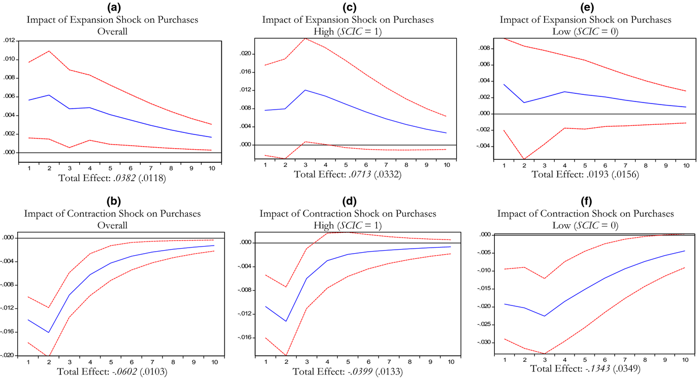
Impulse Response Function of Macro‐economic Shocks on PurchasesNote: X‐Axis—Quarters; Y‐Axis—Purchases; the solid line represents response of purchases to a one SD increase in macroeconomic shocks. The dotted lines represent ±2 SD band

7. Conclusions

The main result of our article is that stockout and inventory holding costs faced by retailers have a significant explanatory power over the observed differences in inventory investment behavior across retailers during economically turbulent periods. Our findings are useful in benchmarking inventory performance of retailers. In addition, suppliers to retailers may mitigate demand‐side risk due to economic shocks by improving forecasting accuracy through clustering or segmenting retailers based on the ratio of their stockout to holding cost. Segmenting customers to develop forecasts for each part has been found to improve forecast accuracy in other contexts (Makridakis et al. 1998, Shlifer and Wolff 1979).

Our article suggests the following venues for future research. First, the supply chain risk management literature has traditionally emphasized supplier selection to mitigate supply‐side risk. Similarly, it would be interesting to consider customer selection as a way to mitigate demand‐side risk during economic shocks. Our findings suggest that the impact of macroeconomic shocks on suppliers would depend on the portfolio of the retailers they serve. Suppliers may be able to pool forecast risks across different types of retailers so that extreme fluctuations in orders are mitigated. Future research may examine if the choice of retailers to serve is a viable supply chain strategy to manage economic risk.

Second, our results suggest future directions to detect the bullwhip effect. Prior empirical research that examines the bullwhip effect tends to aggregate across firms and also time periods and has largely failed to find evidence for this effect. For example, Cachon et al. (2007), who studied this phenomenon using industry‐level data, could not find any evidence of the bullwhip effect in the retail industry. Aggregation of observations across firms without consideration to their stockout and inventory holding costs would attenuate the bullwhip effect at the industry level. Similarly, aggregating across periods of expansion and contraction shocks would lead to an attenuation bias that may make it difficult to detect the bullwhip effect at the industry level. Future research may examine the bullwhip effect separately for different types of retailers and for different types of shocks identified in this article.

Third, our theoretical model and estimation methodology ignore setup costs. Since retailers are likely to make inventory decisions in a multi‐period framework, it would be useful to examine if differences in setup costs across retailers explain differences in inventory investment. Such an exercise would involve the determination of an appropriate measure for setup costs at the firm level.

Fourth, we use gross margin and WACC as proxies for stockout and inventory holding costs, respectively. While we follow previous literature on these measurements, we acknowledge limitations of using such proxies. These proxies may capture other aspects of managerial decision making in addition to the intended variables. For example, the WACC measure may be impacted by several firm decisions such as mergers and acquisitions as well as credit rating. Future research could examine ways to obtain better measures of stockout and holding costs.

Finally, while our study is restricted to estimating the impact of macroeconomic shocks on retailers' inventory level, future research may consider other types of demand shocks and examine how firms manage them. For example, Kesavan et al. (2012) study how high and low inventory turnover retailers follow different ordering and pricing mechanisms to manage idiosyncratic firm‐level demand shocks. In addition, considering terms of the supply chain contracts that exist between retailers and their suppliers could lead to a deeper understanding of factors that drive retailers' response to demand shocks.

Footnotes

Acknowledgments

We are grateful to the following individuals for their helpful feedback: Barry Bayus, Vinayak Deshpande, Andrew Petersen, and Harvey Wagner. Both authors contributed equally and their names appear in alphabetical order.

1

GDP, retail sales, and personal consumption expenditure data are obtained from the Bureau of Economic Analysis and COMPUSTAT.

2

http://www.pginvestor.com/phoenix.zhtml?c=104574&p=irol-newsArticle&ID=1316941

3

Our conversations with the P&G business intelligence group confirmed that the question of how retailers change their inventory investment during recessions is of direct relevance to them.

4

Our empirical testing strategy does not require demand to be normally distributed.

5

We use this definition of shock to be consistent with prior literature (Lamey et al. ). The conceptual reasoning underlying this definition is that, in a manager's or consumer's mind, the current state of the economy is always compared with the previous best or previous worst of the recent times. In addition, this measurement permits us to decompose a shock into expansion and contraction components. We subsequently test robustness to alternate measurement.

6

The cyclical component extracted in the first stage is deterministic rather than stochastic; hence, we do not need to perform bootstrap replications.

7

We compare the market shares, calculated as retailer's revenue for the quarter divided by total revenue of the industry in that quarter, of the dropped retailers (mean = 2.04%, SD = 4.89%) with those that we retain in our sample (mean = 2.16%, SD = 5.91%). Though the small difference is statistically significant at a very large sample size, the effect size is particularly small, thereby enhancing our confidence that the dropped retailers are systematically not much different from those retained in our sample.

8

In an acyclical industry, the industry sales do not significantly co‐vary with the unexpected changes in GDP.

9

In absence of an autoregressive term, the impact of contraction shocks and gross margins is significantly exaggerated, while those of expansion shocks are significantly marginalized. While the substantive findings remain unchanged, the difference in the size of coefficients indicates the bias that would be introduced if we do not include the autoregressive term. This result echoes similar findings in economics and marketing that have shown that ignoring state dependence in aggregate firm‐level variables can lead to significant bias in evaluating the impact of exogenous variables (e.g., see Jacobson 1990). In addition, as discussed in section , we find that specifications with no autoregressive terms have relatively poor model fit. Thus, in interest of maximizing variance explained by maintaining parsimony, we retain the specification with autoregressive term.

10

We choose to retain our proposed ARDL(1,1) specification because including multiple distributed lag terms can introduce severe multicollinearity, thereby inflating the standard errors and hence leading to an incorrect interpretation of the coefficients.

11

Therefore, we do not need to decompose the CCI series into a linear trend and a cyclical component around it.

References

Anderson

Fitzsimons

Simester

. 2006. Measuring and mitigating the costs of stockouts. Manage. Sci. 52(11): 1751–1763.

Anderson

S. T.

Kellogg

Sallee

J. M.

Curtin

R. T.

. 2011. Forecasting gasoline prices using consumer surveys. Am. Econ. Rev. Papers & Proc. 101(3): 110–114.

Bils

Kahn

J. A.

. 2000. What inventory behavior tells us about business cycles. Am. Econ. Rev. 90(3): 458–481.

Blinder

1981. Retail inventory behavior and business fluctuations. Brook. Pap. Econ. Activity 2: 443–520.

Blinder

A. S.

Maccini

L. J.

. 1991. The resurgence of inventory research: What have we learned? J. Econ. Surveys 5(4): 291–328.

Cachon

G. P.

Randall

Schmidt

G. M.

. 2007. In search of the bullwhip effect. Manuf. Ser. Oper. Manag. 9(4): 457–479.

Caplin

A. S.

1985. The variability of aggregate demand with (S,s) inventory policies. Econometrica 53: 1395–1409.

Chen

Frank

M. Z.

O. Q.

. 2005. What actually happened to inventories of American companies between 1981 and 2000. Manage. Sci. 51(7): 1015–1031.

Chen

Frank

M. Z.

O. Q.

. 2007. U.S. retail and wholesale inventory performance from 1981 to 2004. Manuf. Ser. Oper. Manag. 9(4): 430–456.

10.

Chopra

Sodhi

M. S.

. 2004. Managing risks to avoid supply chain breakdowns. Sloan Manage. Rev. 46(1): 53–61.

11.

Clements

M. P.

Galvao

A. B.

. 2009. Forecasting U.S. output growth using leading indicators: An appraisal using MIDAS models. J. Appl. Econom. 24(7): 1187–1206.

12.

Cochrane

J. H.

1994. Shocks. Carnegie‐Rochester Conference Series on Public Policy 41: 295–364.

13.

Cover

J. P.

1992. Asymmetric effects of positive and negative money‐supply shocks. Quart. J. Econ. 107(4): 1261–1282.

14.

Davidson

MacKinnon

J. G.

. 1993. Estimation and Inference in Econometrics. Oxford University Press, New York.

15.

Dopke

Fritsche

. 2006. When do forecasters disagree? An assessment of German growth and inflation forecast dispersion. Int. J. Forecast. 22(1): 125–135.

16.

Dovern

Fritsche

Slacalek

. 2012. Disagreement among forecasters in G7 countries. Rev. Econ. Stat. Forthcoming 94(4): 1081–1096.

17.

Edison

H. J.

Pauls

B. D.

. 1993. A re‐assessment of the relationship between real exchange rates and real interest rates: 1974–1990. J. Monet. Econ. 31(2): 165–187.

18.

Garvin

D. A.

Edmondson

A. C.

Gino

. 2008. Is yours a learning organization? Harv. Bus. Rev. 86(3): 109–116.

19.

Gaur

Fisher

M. L.

Raman

. 2005a. An econometric analysis of inventory turnover performance in retail services. Manage. Sci. 51(2): 181–194.

20.

Gaur

Giloni

Seshadri

. 2005b. Information sharing in a supply chain under ARMA demand. Manage. Sci. 51(6): 961–969.

21.

Gaur

Kesavan

. 2009. The effects of retailer size and sales growth rate on inventory turnover performance in U.S. retail services. Agrawal

Smith

, eds. Retail Supply Chain Management. Springer, New York, 25–52.

22.

Gaur

Kesavan

Raman

Fisher

. 2007. Estimating demand uncertainty using judgmental forecasts. Manuf. Ser. Oper. Manag. 9(4): 480–491.

23.

Gurnani

Mehrotra

Ray

. 2012. Supply Chain Disruptions: Theory and Practice of Managing Risks. Springer, New York.

24.

Hendricks

K. B.

Singhal

V. R.

. 2005. An empirical analysis of the effect of supply chain disruptions on long‐run stock price performance and equity risk of the firm. Prod. Oper. Manag. 14(1): 25–53.

25.

Hendricks

K. B.

Singhal

V. R.

. 2012. Supply chain disruptions and corporate performance. Gurnani

Mehrotra

Ray

, eds. Supply Chain Disruptions: Theory and Practice of Managing Risks. Springer, New York, 1–20.

26.

Hodrick

R. J.

Prescott

E. C.

. 1997. Postwar U.S. business cycles: An empirical investigation. J. Money. Credit. Bank. 29: 1–16.

27.

Irvine

F. O.

Jr . 1981. Retail inventory investment and the cost of capital. Am. Econ. Rev. 71: 633–668.

28.

Jacobson

R. D.

1990. Unobservable effects and business performance. Mark. Sci. 9(1): 74–85.

29.

Kahn

J. A.

1987. Inventories and the volatility of production. Am. Econ. Rev. 77: 667–669.

30.

Kahn

J. A.

1992. Why is production more volatile than sales? Theory and evidence on the SC‐avoidance motive for inventory‐holding. Quart. J. Econ. 107(2): 481–510.

31.

Kalaignanam

Kushwaha

Eilert

. 2013. The impact of product recalls on future product reliability and future accidents: Evidence from the automobile industry. J. Mark. Forthcoming 77(2): 41–57.

32.

Kamakura

. 2012. How economic contractions and expansions affect expenditure patterns. J. Consum. Res. 39(3): 229–247.

33.

Karlin

Fabens

. 1959. The (s, S) inventory model under Markovian demand process. Arrow

Karlin

Suppes

, eds. Mathematical Methods in the Social Sciences. Stanford University Press, Stanford, CA, 159–175.

34.

Kesavan

Gaur

Raman

. 2010. Do inventory and gross margin data improve sales forecasts for U.S. public retailers? Manage. Sci. 56(9): 1519–1533.

35.

Kesavan

Kushwaha

Gaur

. 2012. Do high‐ and low‐ inventory turnover retailers respond differently to demand shocks? Working paper, University of North Carolina at Chapel Hill.

36.

Kesavan

Mani

. 2013. The relationship between abnormal inventory growth and future earnings for U.S. public retailers. Manuf. Ser. Oper. Manag. 15(1): 6–23.

37.

Khan

Thomas

J. K.

. 2007. Inventories and business cycles: An equilibrium analysis of (S, s) policies. Am. Econ. Rev. 97(4): 1165–1188.

38.

Lamey

Deersnyder

Dekimpe

M. G.

Steenkamp

J. B. E. M.

. 2007. How business cycles contribute to private‐label success: Evidence from the U.S. and Europe. J. Mark. 71(1): 1–15.

39.

Lamey

Deersnyder

Steenkamp

J. B. E. M.

Dekimpe

M. G.

. 2012. The effect of business cycle fluctuations on private‐label share: What has marketing conduct got to do with it? J. Mark. 76(1): 1–19.

40.

Maccini

Rossana

R. J.

. 1981. Investment in finished goods inventories: An analysis of adjustment speeds. Am. Econ. Rev. 71(2): 17–22.

41.

Makridakis

Wheelwright

Hyndman

R. J.

. 1998. Forecasting: Methods and Applications. John Wiley and Sons, New York.

42.

Mankiw

N. G.

Reis

Wolfers

. 2004. Disagreement about inflation expectations. NBER Macroeconomics Annual Report 18: 1–60.

43.

Mitra

Golder

. 2006. How does objective quality affect perceived quality: Short‐term effects, long‐term effects, and asymmetries. Mark. Sci. 25(2): 230–247.

44.

Nerlove

1958. Adaptive expectations and cobweb phenomena. Quart. J. Econ. 72(2): 227–240.

45.

Pesaran

M. H.

Shin

. 1998. Generalized impulse response analysis in linear multivariate models. Econ. Lett. 58(1): 17–29.

46.

Petruzzi

N. C.

Dada

. 1999. Pricing and the newsvendor problem: A review with extensions. Oper. Res. 47(2): 183–194.

47.

Rajagopalan

2012. Impact of variety and distribution system characteristics on inventory levels at US retailers. Manuf. Ser. Oper. Manag. Forthcoming 15(2): 27–40.

48.

Raman

Kim

. 2002. Quantifying the impact of IC and reactive capacity on an apparel manufacturer's profitability. Prod. Oper. Manag. 11(3): 358–373.

49.

Ravn

M. O.

Uhlig

. 2002. On adjusting the Hodrick‐Prescott filter for the frequency of observations. Rev. Econ. Stat. 84(2): 371–375.

50.

Rumyantsev

Netessine

. 2007. What can be learned from classical inventory models? A cross‐industry exploratory investigation. Manuf. Ser. Oper. Manag. 9(4): 409–429.

51.

Sethi

Cheng

. 1997. Optimality of (s, S) policies in inventory models with Markovian demand. Oper. Res. 45(6): 931–939.

52.

Shlifer

Wolff

R. W.

. 1979. Aggregation and proration in forecasting. Manage. Sci. 25(6): 594–603.

53.

Sims

C. A.

1980. Macroeconomics and reality. Econometrica 48(1): 1–48.

54.

Song

J. S.

Zipkin

. 1993. Inventory control in a fluctuating demand environment. Oper. Res. 41(2): 351–370.

55.

Tang

C. S.

2006. Perspectives in supply chain risk management. Int. J. Prod. Econ. 103: 451–488.

56.

Thoma

M. A.

1994. Subsample instability and asymmetries in money‐income causality. J. Econom. 64(1): 279–306.

57.

Wen

2005. Understanding the inventory cycle. J. Monet. Econ. 52(8): 1533–1555.

Variable	Overall		High service level		Low service level
Variable	Mean	SD	Mean	SD	Mean	SD
INVT ($)	226.124	484.846	226.444	455.238	225.661	524.814
MRGN (%)	57.140	12.002	60.289	9.897	52.580	13.255
WACC (%)	1.581	1.823	0.762	0.399	2.460	2.286
SCIC	97.784	576.249	168.809	926.677	26.723	110.532
SHOCK ^EXP (%)	0.829	0.544
SHOCK ^CONT (%)	0.949	1.170
COGS ($)	226.235	531.640	220.785	514.101	234.129	556.012
AT ($)	688.555	1513.651	690.046	1456.923	686.394	1592.357
Days payable (DP)	79.830	51.492	88.707	52.155	66.965	47.671

Dependent variable—ΔLINVT _it	Expansion		Contraction
Dependent variable—ΔLINVT _it	Coeff.	SE	Coeff.	SE
ΔLINVT _it−1 *	0.419	0.026	0.458	0.022
ΔLMRGN _it *	0.346	0.082	0.176	0.055
ΔLSALES _it *	0.474	0.059	0.405	0.043
ΔLDP _it *	0.054	0.027	0.150	0.022
ΔLAT _it *	0.105	0.039	0.121	0.029
${SHOCK}_{t}^{Exp}$	1.867	0.699
${SHOCK}_{t - 1}^{Exp}$	−0.917	0.677
${SHOCK}_{t}^{Cont}$			−1.075	0.572
${SHOCK}_{t - 1}^{Cont}$			0.305	0.680
Intercept	−0.043	0.019	−0.015	0.007
Quarter effects	Three significant		One significant
Industry segment effects	None significant		One significant
	H1a		H1b
Short‐term effects	0.950	0.347	−0.770	0.250
Long‐term effects	1.636	0.597	−1.420	0.458
Sample size N (No. of retailers)	4357 (355)		5059 (360)
R ² total	0.638		0.675

	H2a Expansion		H2b Contraction
	Diff	SE	Diff	SE
Short‐term effects (high−low)	1.099	0.507	0.821	0.346
Long‐term effects (high−low)	1.960	0.904	1.482	0.587