Inventory Rationing in a Make‐to‐Stock System with Batch Production and Lost Sales

Abstract

We address an inventory rationing problem in a lost sales make‐to‐stock (MTS) production system with batch ordering and multiple demand classes. Each production order contains a single batch of a fixed lot size and the processing time of each batch is random. Assuming that there is at most one order outstanding at any point in time, we first address the case with the general production time distribution. We show that the optimal order policy is characterized by a reorder point and the optimal rationing policy is characterized by time‐dependent rationing levels. We then approximate the production time distribution with a phase‐type distribution and show that the optimal policy can be characterized by a reorder point and state‐dependent rationing levels. Using the Erlang production time distribution, we generalize the model to a tandem MTS system in which there may be multiple outstanding orders. We introduce a state‐transformation approach to perform the structural analysis and show that both the reorder point and rationing levels are state dependent. We show the monotonicity of the optimal reorder point and rationing levels for the outstanding orders, and generate new theoretical and managerial insights from the research findings.

Keywords

production and inventory control inventory rationing batch production make‐to‐Stock

Introduction

Inventory rationing among multiple customer classes (segments) lies at the heart of the yield management problem (Deshpande et al. 2003). It is an important tactic for coordinating demand management and inventory control in many industries where the service level requirements vary widely among demand classes. For example, Cohen et al. (1988) study service parts management with priority demand classes in the computer industry where a retailer could place either regular orders or emergency orders. Deshpande et al. (2003) provide an example of inventory rationing in the US military. Another example is Dell Computer, which segments customers by type (e.g., family, industry, government, academic, etc.) and sells the same product (computers) to different segments at different prices (McWilliams 2001). Similar problems also exist in service industries with fixed and perishable capacity (e.g., airlines, car rentals, hotels, etc.) where the critical decisions include the prices charged to demand classes and the rationing levels (see, e.g., Kimes 1989, Talluri and van Ryzin 2004). Kleijn and Dekker (1999) provide an overview of the inventory rationing problem and present applications ranging from airlines to petrochemical firms.

Our study aims to address several salient features that are commonly observed in the inventory management of many production and supply systems. First, demand is uncertain and can be segmented into multiple classes according to customers' willingness to pay and their service level requirements. Second, the production and supply processes may consist of multiple sequential phases with uncertain delivery lead times. For example, an in‐house production system may have a sequential production process that includes raw materials processing, work‐in‐process component processing, assembly, inspection, and packaging. A typical supply system of a global firm may consist of multiple sequential delivery stages including order processing, multi‐phase shipping, and custom clearance. The end customer demand and the time required to complete each stage and the whole process may fluctuate over time. See Zipkin (2000) for more discussions on sequential supply systems. Third, replenishment orders are often restricted to fixed batch sizes (i.e., full truck loads or containers).

In this study we consider an inventory rationing problem of a continuous review make‐to‐stock (MTS) system with batch production and multiple demand classes. Demands arrive according to Poisson processes. Unmet demand is lost and a penalty cost is incurred. For any incoming customer order, the system manager determines whether to satisfy it with on‐hand inventory (if there is any) or reject it. The demand classes have different values for the same product, which are represented by class‐specific prices and penalty costs for lost sales (or shortages). Each production order contains a single batch of a fixed lot size (e.g., in a full truckload or a full container). The production processing time is random. The objective of the system is to maximize the total discounted profit over an infinite horizon.

We formulate the problem as a Markov decision process (MDP). We first address the case where the production times are generally distributed and there is at most one outstanding order. We show that the optimal ordering policy can be characterized by a critical stock level. That is, the reorder point policy is optimal. The inventory rationing control for each demand class is characterized by time‐dependent critical stock levels, also called rationing levels. We show that the rationing levels are decreasing in the elapsed production time of the outstanding order. Since it is difficult to further generalize the structural analysis under general production times to the case that allows multiple outstanding orders, we approximate the production time distribution with a phase‐type distribution and show that the optimal policy can be characterized by a reorder point and state‐dependent rationing levels. We then use a tandem MTS system to address the issue of allowing multiple outstanding orders. Assuming that the production time follows an Erlang distribution, we show that both the reorder point and inventory rationing levels are state dependent. We characterize the monotonicity of the optimal reorder point and rationing levels for the pipeline of outstanding orders and discuss the managerial insights. The numerical results show that when the batch size is relatively large it may be sufficient to restrict the system to allow at most one order outstanding.

Our contributions are two twofold. First, we generalize the lost sales inventory rationing models to batch‐ordering systems while allowing multiple orders outstanding simultaneously. The intrinsic difficulty in analyzing the lost sales system with multiple orders outstanding arises from the fact that the decision maker needs to take into account the status of all the outstanding orders while making inventory replenishment and rationing decisions. Second, when addressing the case with multiple outstanding orders, we introduce a state‐transformation approach to treat the system as a serial system. This approach enables us to tackle the multi‐outstanding‐order problem and provide new insights into the inventory rationing problem. We show that when an order is placed, the subsequent reorder point decreases, but will increase in the time since the order was placed. This has the effect of decreasing the likelihood of placing a second order until such time when the first order is more likely to arrive. Conversely, we show that the rationing levels decrease in the time since the order was placed. This implies that when an order is placed, little changes in the rationing policy, but as the order arrival approaches, the rationing levels fall to ensure that excess inventory is removed prior to the arrival of the order. To the best of our knowledge, these structural results are shown for the first time for batch production inventory rationing problems.

The remainder of this article is organized as follows. Section 2 reviews the related literature. Section 3 addresses the case with general production times and a single outstanding order and approximates the general production time distributions with phase‐type distributions. Section 3 generalizes the analysis to the case with multiple outstanding orders. Section 5 provides the concluding remarks. All the proofs are placed in Appendix S1.

Related Literature

This study follows the growing literature on the inventory rationing problem initiated by Veinott (1965). See Ding et al. (2006), Arslan et al. (2007), Möllering and Thonemann (2008), Fadiloglu and Bulut (2010), and Cheng et al. (2011) for comprehensive reviews of recent developments. Our study fits into the stream of continuous‐review MTS models with lost sales. The most related works in this literature are Ha (1997, 2000), Melchiors et al. (2000), and Melchiors (2001).

Ha (1997) considers a MTS production system with several demand classes and lost sales. He shows that the critical‐level policy is optimal. Ha (2000) extends Ha (1997) to the case with Erlang distributed production times. Assuming that each production order contains a unit of product and there is only one outstanding order at any point in time, Ha (2000) finds that by combining the two state variables—inventory level and status of the outstanding order—into a single dimensional state, called work storage, the structural results can be readily obtained by backward induction. His results give some insights into the inventory rationing problem by incorporating production status information into the inventory allocation decision, but application of his model is relatively limited due to the restrictive assumptions of unit production and single outstanding order. He points out that one direction important future research is to address the general production time distributions. Our study not only address his concern on the general production time distribution but also further generalizes the model to allow batch production. Note that his approach of work storage state variable aggregation no longer works in our model. Moreover, with Erlang distribution lead times, we allow multiple orders outstanding simultaneously.

Melchiors et al. (2000) consider an (Q, R) inventory system with lost sales and two priority demand classes, under the assumptions of unit Poisson demand, deterministic constant lead times, and at most one order outstanding. They introduce a lead time–independent critical‐level policy, derive the exact formulation of the average cost, and propose a simple optimization procedure. Melchiors (2001) extends the model of Melchiors et al. (2000) to multiple demand classes with generally distributed replenishment lead times. He analyzes the rationing policy for an (R, Q) system with exogenously given reorder point R and order size Q, where R < Q. He shows that the optimal rationing policy can be characterized by time‐dependent critical stock levels. Note that the restriction R < Q implies that there is at most one order outstanding at any point in time. For the case of constant lead times, he shows that the optimal critical levels are a decreasing function of the elapsed lead time of the outstanding order. He does not analyze the optimality of the reorder point policy or the (R, Q) policy. In this study we also consider a batch production system with an exogenously given batch size. However, our model differs from Melchiors (2001) in that the reorder policy is endogenously determined, although it turns out that the optimal production policy can be characterized by a critical reorder point when there is at most one order outstanding at any point in time. Note that the single‐outstanding‐order assumption does not imply R < Q. Nevertheless, when the production times are approximated by a phase‐type distribution, we are able to generalize the model with a single outstanding order to the case with multiple outstanding orders and show that the state‐dependent reorder point policy is optimal.

When there is only one demand class, the inventory rationing model of the (Q, R) system reduces to the traditional (Q, R) model (see, e.g., Hadley and Whitin 1963). For tractability, it is often assumed that there is at most one order outstanding (see, e.g., Buchanan and Love 1985, Hill and Johansen 2004, Nahmias and Demmy 1981). Johansen and Thorstenson (2004) attempt to generalize the lost sales (Q,R) model to the case where more than one order may be outstanding. Assuming that orders do not cross over time, they obtain the equilibrium equations for the underlying MDP and develop a computational algorithm. Different from them, we focus on characterizing the optimal policy structure for an inventory rationing problem with a fixed order batch size, assuming the production times follow an Erlang distribution and allowing multiple outstanding orders.

Also related is the joint pricing and inventory control literature, see, e.g., Elmaghraby and Keskinocak (2003) and Chen and Simchi‐Levi (2012) for comprehensive reviews. Both pricing and rationing are typical marketing instruments for demand management. Chen et al. (2006, 2009) address the joint pricing and production control problem for the unit and batch (exponential) production system, respectively. Pang and Chen (2010) generalize Chen et al. (2009) to the case with Erlangian lead times and two outstanding orders. But their analysis cannot be readily extended to the more general case that allows any number of outstanding orders. We address the multiple outstanding orders issue. Employing a state‐transformation approach, we are able to characterize the structural properties of the optimal policies.

Single Outstanding Order

The Model with General Production Times

Consider a single‐facility MTS production system that offers a single product to N demand classes (subscript

i \in N \equiv {1, \dots, N}

) over an infinite horizon. Demands from different classes arrive according to independent Poisson processes with an arrival rate λ _i for class i customers. When a customer from class i arrives to the system and requests a unit of the product, the system manager must decide whether to accept or reject the demand request. If the request is accepted, then the customer pays a fixed price of p _i per unit of the product. If it is rejected, then the demand is lost and a lost sales cost, π _i, is incurred. The lost sales cost can be interpreted as a direct rebate that the system pays to a customer for not satisfying their demand or a loss of goodwill. It can also represent the loss due to spot purchase, which is equal to the spot price less the sales price. If a class i customer arrives when the system is out of stock, then the demand is lost and the lost sale cost π _i is incurred. That is, the demand classes are differentiated by the prices paid for the product and the lost sales costs. We assume that

π_{1} + p_{1} > \dots > π_{N} + p_{N} .

The product is produced in batches with a fixed lot size Q, an exogenously given positive integer (e.g., a truck load or a full container). This treatment with a (exogenously given) fixed ordering lot size is common in the literature (see, e.g., Chen 2000, Song 2000). The production of each batch incurs a fixed cost, C _f > 0, and a variable cost c per unit. The fixed cost includes administrative costs, transportation costs, and fixed payments to the supplier. So the total cost of each production order is C = C _f + c·Q. We assume that the payment occurs when an order is completed.

The production processing time of each batch, τ, is assumed to be generally distributed with probability density function f and distribution function F. Deterministic production time can be seen as a special case. When τ is a positive random variable, we assume that the failure rate function

ρ (s) = \frac{f (s)}{1 - F (s)}

is strictly increasing. Note that the family of increasing failure rate distributions includes the uniform, exponential, Erlang, normal, truncated normal distributions, etc. (Porteus 2002). The rationale behind this assumption is that as time goes by the outstanding production order will be more likely to arrive. Zipkin (1986) provides a detailed discussion of stochastic lead times in inventory models.

In this section, we assume that at any point in time there is at most one batch being processed in the facility. This assumption ensures that at the time before an order is placed, the inventory position and the net inventory level coincide. Although this assumption is rather restrictive, it provides mathematical tractability while preserving the major characteristics of batch production systems. We refer to Hadley and Whitin (1963), Nahmias and Demmy (1981), and Berk and Gürler (2008) for a similar treatment in the analysis of lost sales (Q, R) inventory systems.

The system state is described by a two‐dimensional state variable (X(t), S(t)), where

X (t) \in Z_{+}

is the inventory level at time t and S(t) is the elapsed processing time of the outstanding order (if there is any). In other words, S(t) records the age of the outstanding order. If there is no outstanding order or an outstanding order is completed at time t, then S(t) = 0. At any time t, when the current state is (x, s), a joint decision needs to be made on production and inventory allocation. In particular, when there is no ongoing production (s = 0), the system manager needs to decide both whether to place a production order and whether to accept an incoming demand order. When there is an order outstanding (s > 0), the manager needs only to determine whether to accept an incoming demand order.

Different from the system where the transition time between each two consecutive inventory states is exponentially distributed (see, e.g., Ha 2000), the transitions of inventory states in our model are not time memoryless since the transitions depend on the elapsed time (or age) of the outstanding order (if there is any). Let

U

be the set of admissible policies. A policy

u \in U

can be specified as u(t) = {u ₀(X(t),S(t)),u ₁(X(t),S(t)),⋯,u _N(X(t),S(t))}, where u ₀(x,0) = 0, if there is no order outstanding and no new order is placed, u ₀(x,0) = 1, if there is no order outstanding and a new order is placed, u _n(x,s) = 1, if an incoming customer order of class n is accepted, and u _n(x,s) = 0, if an incoming customer order of class n is rejected. Let

D_{n}^{u} (t)

denote the accumulated sales from class n customers,

L_{n}^{u} (t)

the accumulated lost sales to class n customers, and P ^u(t) the number of batches produced (received) up to t under the policy u. Then, we have

X^{u} (t) = X (0) + Q P^{u} (t) - \sum_{n = 1}^{N} D_{n}^{u} (t)

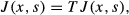
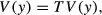
The objective of the system is to find the optimal control policy u ^* that maximizes the expected discounted profit over an infinite horizon:

J_{γ}^{u^{*}} (x, s) = max_{u \in U} E_{t} [\int_{0}^{\infty} e^{- γ t} (\sum_{n = 1}^{N} p_{n} d D_{n}^{u} (t) - C d P^{u} (t) - \sum_{n = 1}^{N} π_{n} d L_{n}^{u} (t) - h X^{u} (t) d t)],

(1)

where γ > 0 is the discount factor, (x,s) is the initial state, and

E_{t} [\cdot] = E [\cdot | (X (0), S (0)) = (x, s)]

. For convenience, we let

J = J_{γ}^{u^{*}}

Let Δ be a positive small interval and

Λ = \sum_{n = 1}^{N} λ_{n}

. Given any state (x,s), s > 0, the first‐order probability that the production will be completed in time (s,s + Δ) is

\frac{f (s)}{1 - F (s)} Δ

. The probability that a customer of class n arrives in (s,s + Δ) is λ _nΔ. Assume that Δ is sufficiently small such that (γ + Λ + ρ(s))Δ < 1 for all s ≥ 0.

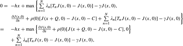
By Bellman's principle, we have

J (x, s) = T J (x, s),

(2)

where the operator T is defined on functions

v : Z_{+} \times R_{+} \to R

such that

T v (x, s) = - h x Δ + \{\begin{matrix} max \{\hat{T} v (x, 0), \tilde{T} v (x, 0)\} + o (Δ), i f s = 0 \hat{T} v (x, s) + o (Δ), if s > 0 \end{matrix},

(3)

\tilde{T} v (x, 0) = \sum_{n = 1}^{N} λ_{n} Δ T_{n} v (x, 0) + (1 - γ Δ - Λ Δ) v (x, 0),

(4)

\begin{matrix} \hat{T} v (x, s) = & ρ (s) Δ [v (= x + Q, 0) - C] \\ + (1 - ρ (s) Δ) [\sum_{n = 1}^{N} λ_{n} Δ T_{n} v (x, s + Δ) + (1 - γ Δ - Λ Δ) v (x, s + Δ)] + o (Δ), \\ = ρ (s) Δ [v (x + Q, 0) - v (x, s + Δ) - C] \\ + [\sum_{n = 1}^{N} λ_{n} Δ T_{n} v (x, s + Δ) + (1 - γ Δ - Λ Δ) v (x, s + Δ)] + o (Δ), \end{matrix}

(5)

\begin{matrix} T_{n} v (x, s) = & max {p_{n} + v (x - 1, s), v (x, s) - π_{n}} 1_{{x > 0}} \\ + [v (x, s) - π_{n}] 1_{{x = 0}} . \end{matrix}

(6)

Note that the operator

\hat{T}

corresponds to the ordering decision and

\tilde{T}

corresponds to the decision of placing no order. Given a state (x,0), it is optimal to place an order if

\hat{T} J (x, 0) > \tilde{T} J (x, 0)

. The operator T _n is associated with the admission control of whether to accept or reject orders from customers of class n. For any state (x, s), the optimal demand rate from demand class n is defined as

λ_{n} (x, s) \equiv λ_{n} 1_{{D J (x, s) < p_{n} + π_{n}}},

(7)

where the operator D of a function v(x,i) is defined as

\begin{matrix} D v (x, s) & = v (x, s) - v (x - 1, s) and \\ D^{2} v (x, s) & = D v (x, s) - D v (x - 1, s) . \end{matrix}

Here, Dv(x, s) measures the marginal loss of reducing one unit of inventory in state (x, s). We call it the marginal value or shadow price of the inventory.

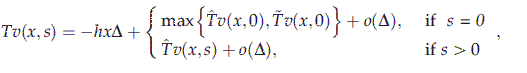
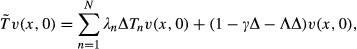
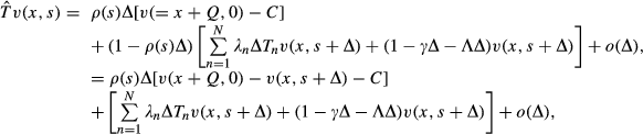
Re‐arranging the terms, dividing both sides by Δ, and letting Δ → 0 yields the HJB equations: If s = 0,

\begin{matrix} 0 = & - h x + max \{\sum_{n = 1}^{N} λ_{n} [T_{n} J (x, 0) - J (x, 0)] - γ J (x, 0), \\ \frac{\partial J (x, 0)}{\partial s} + ρ (0) [J (x + Q, 0) - J (x, 0) - C] + \sum_{n = 1}^{N} λ_{n} [T_{n} J (x, 0) - J (x, 0)] - γ J (x, 0)\} \\ = & - h x + max \{\frac{\partial J (x, 0)}{\partial s} + ρ (0) [J (x + Q, 0) - J (x, 0) - C], 0\} \\ + \sum_{n = 1}^{N} λ_{n} [T_{n} J (x, 0) - J (x, 0)] - γ J (x, 0), \end{matrix}

(8)

and if s > 0,

0 = - h x + \frac{\partial J (x, s)}{\partial s} + ρ (s) [J (x + Q, 0) - J (x, s) - C] + \sum_{n = 1}^{N} λ_{n} [T_{n} J (x, s) - J (x, s)] - γ J (x, s),

(9)

where

\frac{\partial J (x, 0)}{\partial s} = {lim}_{Δ \to 0 +} \frac{J (x, Δ) - J (x, 0)}{Δ}

. Note that as s = 0, a production order is placed if

\frac{\partial J (x, 0)}{\partial s} + ρ (0) [J (x + Q, 0) - J (x, 0) - C] > 0 .

This is consistent with its first‐order approximation 2 because

lim_{Δ \to 0} \frac{\hat{T} J (x, 0) - \tilde{T} J (x, 0)}{Δ} = \frac{\partial J (x, 0)}{\partial s} + ρ (0) [J (x + Q, 0) - J (x, 0) - C] .

Structure of the Optimal Policy

It is difficult to analyze the solutions of differential equation systems 8 and 9 directly. In the following analysis we perform backward induction on the first‐order approximate optimality equation 2. For convenience, we omit the notation o(Δ) in the analysis.

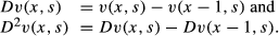
We first define a set of structural functions. Let

V

be the set of functions defined on

Z_{+} \times R_{+}

such that for any

v \in V, Δ > 0,

and s ≥ 0,

(C1)

Dv(x + Q,0) ≤ Dv(x,s) and Dv(x,s + Δ) ≤ Dv(x,s).

(C2)

Dv(x,s) < p ₁ + π ₁.

(C3)

{lim}_{x \to \infty} D v (x, s) = - \frac{h}{γ} .

These properties partially characterize the structural properties of the optimal value function. The first inequality (C1) implies that the opportunity cost of each outstanding batch order v(x + Q,0) − v(x,s) is decreasing in the inventory level x for any s ≥ 0. This property is also called Q‐difference decreasing (Huh and Janakiraman 2012). The second inequality (C1) states that the marginal value of inventory on hand is decreasing in the age of the outstanding order, which implies that

\frac{\partial D v (x, s)}{\partial s} \leq 0

. As we will show below, these two properties allow us to characterize the structure of the optimal production control policy. Property (C2) states that the marginal value of inventory is always smaller than the benefit of accepting a customer order of the highest priority class 1, which implies that the customer orders of the highest priority class are always accepted. Property (C3) shows the limiting behaviour of the marginal value of inventory when the inventory level is sufficiently high. This property and the first inequality (C1) together provide a lower bound on the marginal value of inventory.

Lemma 1

J \in V

Lemma 1 employs the backward induction approach on the Bellman equation to establish some structural properties of the optimal profit function. To completely characterize the structure of the joint production control and inventory rationing policy requires the concavity property with respect to the inventory level. We are not able to prove concavity via the backward induction approach. Fortunately, we find that concavity can be proved by using the properties of Lemma 2 and manipulating the HJB equations 8 and 9.

Lemma 2

For any s ≥ 0, J(x,s) is concave in x, i.e., D ² J(x,s) ≤ 0 for all x ≥ 2.

We now characterize the structure of the optimal policy

Theorem 1

The optimal production control policy is characterized by a critical stock level (reorder point):

R = min \{x \in Z_{+} : \frac{\partial J (x, 0)}{\partial s} + ρ (0) [J (x + Q, 0) - J (x, 0) - C] \leq 0\} - 1,

at or below which it is optimal to place an order (of a batch of size Q) if there is no outstanding order (i = 0); otherwise, it is optimal to place no order. Moreover, R < ∞.

The optimal rationing policy can be characterized by the time‐dependent critical levels:

K_{n} (s) = max {x \in Z_{+} : D J (x, s) \geq p_{n} + π_{n}}, s \geq 0, n = 1, \dots, N - 1,

such that for any s, it is optimal to satisfy a class n demand if the inventory level is above or equal to K _n(s) and reject it otherwise. Moreover, the time‐dependent critical levels satisfy

0 = K_{1} (s) \leq K_{2} (s) \leq \dots \leq K_{N - 1} (s),

and

K_{n} (s + Δ) \leq K_{n} (s), \forall Δ \geq 0, n = 1, \dots, N - 1 .

In Theorem 1, part (a) shows that the optimal batch production control policy is of the critical‐level type. Thus, the reorder point policy is optimal.

Part (b) states that for any class n demand, the optimal rationing policy is characterized by the time‐dependent critical level K _n(s) when s units of time have elapsed. If the inventory level is below or at K _n(s), the marginal value of inventory exceeds the penalty cost plus the lost sales revenue due to rejecting the customer order. In other words, when the inventory level is low, it is more beneficial to reserve inventory in anticipation of future demands from higher priority classes. When the inventory level is high, it is more beneficial to accept more orders from lower priority demand classes so as to increase the total revenue and reduce the inventory holding cost. In particular, the marginal value of inventory is always less than p ₁ + π ₁, which implies that it is always optimal to accept class 1 customer orders, i.e., K ₁(s) = 0.

For any s, K _n(s) is increasing in n. This nested threshold structure implies that the higher the inventory level is, the more demands from lower priority classes will be accepted. For any n, K _n(s) is decreasing in s, which follows from property (C1). The rationale behind the time‐monotone structure is as follows: When making an inventory allocation (rationing) decision, the manager needs to take into account not only the inventory position (= on‐hand inventory + inventory being processed) but also the status of production. As time goes by, the outstanding order gets closer to completion, so the opportunity cost of on‐hand inventory becomes lower (due to the incoming production order). Thus, given the same inventory position, the state with a production order closer to completion tends to accept more lower priority customer orders.

The threshold type of policy structure characterized by Theorem 2 is very intuitive and easy to implement. It is in line with that of Ha (2000) for systems with unit production and Erlangian production times. However, it is worth mentioning that the analysis of the batch production system is technically more challenging because Ha's approach of aggregating the two‐dimensional state space into a one‐dimensional state space no longer works in our model. In addition, the system with a batch‐ordering restriction normally does not have the concavity property (see Huh and Janakiraman 2012). Without the concavity property, the rationing control policy may not be of the threshold type. Hence, this nice property is a surprise to us and it allows us to have a complete characterization of the rationing policy.

Our analysis benefits from the assumptions of Poisson demand, lost sales, and a single outstanding order. In particular, when allowing multiple outstanding orders, with generally distributed lead times, the model becomes intractable since there may be an infinite number of outstanding orders at any point in time. In the following analysis, we first use a phase method to approximate the production times and then extend the structural analysis to the case that allows multiple outstanding orders.

Approximation with Phase‐Type Distributions

The exact computation of the above model with general production time distribution, although possible, is not easy, as it involves solving a differential equation system. It is known that it is possible to approximate any distribution on non‐negative real numbers by a phase‐type (PH) distribution to any degree of accuracy (Tijms 1994). Using the PH distribution to approximate the general distribution is also called the method of phases in queueing theory. This method is often used in inventory theory to model stochastic lead times (Zipkin 1988, 2001). A typical class of PH distributions is the mixed‐Erlang distribution. Many distributions, such as the exponential distribution, Erlang distribution, and hyper‐exponential distribution, are special cases of the mixed‐Erlang distribution. Therefore, we can use the mixed‐Erlang distributed processing times to approximate general stochastic lead times. The advantage of using the mixed‐Erlang distribution is that the duration of each delivery phase is exponential. Since the demand processes are Poisson processes, the system is memoryless when it is between two delivery phases or two consecutive demand arrivals, which enables us to easily work on the Markovian discrete event system and compute the optimal policies.

Approximating the production time distribution using the mixed‐Erlang distribution is natural for systems with the following operational characteristics: The production process consists of multiple processing steps. The duration of each step is approximately exponentially distributed, and the number of steps to finish the production of each batch is random. Then, each Erlangian phase corresponds to a production step, and the completion of each phase corresponds to the completion of each production step. See Ha (2000) for detailed justifications for using phases to represent partially completed production.

In the following analysis, we assume that the production times follow the following distribution:

F = \sum_{m = 1}^{k} ω_{m} E r (m, β),

where k is a positive integer,

\sum_{m = 1}^{k} ω_{m} = 1

, and Er(m,β) is an Erlang distribution with m phases and each phase is exponentially distributed with a mean 1/β. In particular, when ω _k=1, the production times follow a k‐phase Erlang distribution, which can approximate deterministic production times when k is sufficiently large. Given the number of completed phases i, the residual production time satisfies the distribution

F^{(i)} = \sum_{m = i + 1}^{k} \frac{ω_{m}}{\sum_{j = i + 1}^{m} ω_{j}} E r (m - i, β)

, i = 1, …, k − 1.

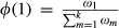
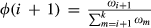
Tijms (1994) demonstrates how to approximate a general distribution using the mixed‐Erlang distribution. For example, when 0 ≤ c _τ ≤ 1, where c _τ is the coefficient of variation in the production time τ, the distribution of τ can be approximated by a mixture of two Erlang distributions with k and k − 1 phases with probabilities ω and 1 − ω, respectively, and the same rate β such that

1 / k \leq c_{τ}^{2} \leq 1 / (k - 1)

. By matching the means and coefficients of variation of the distribution of τ and the approximate mixed‐Erlang distribution, Tijms (1994) shows that the parameters of the mixed‐Erlang distribution can be estimated as

ω = \frac{1}{1 + c_{τ}^{2}} [k c_{τ}^{2} - {(k (1 + c_{τ}^{2}) - k^{2} c_{τ}^{2})}^{1 / 2}], β = \frac{k - ω}{E [τ]} .

(10)

We refer to Tijms (1994) for more detailed discussions on how to approximate general distribution with phase‐type distributions.

With mixed Erlangian processing times, the state of the system can be represented by

(x, i) \in Z_{+} \times Z_{+}

, where x refers to the inventory level and i represents the number of completed phases. In particular, i = 0 refers to the production status that there is no ongoing production. If a production order is placed, then it will be completed in the next phase with probability

ϕ (1) = \frac{ω_{1}}{\sum_{m = 1}^{k} ω_{m}}

and for any i ≥ 0,

ϕ (i + 1) = \frac{ω_{i + 1}}{\sum_{m = i + 1}^{k} ω_{m}}

. We assume that ϕ(i) is increasing in i ≥ 1 and ϕ(k) = 1. This assumption implies that, as time goes by, the probability that the ongoing production will be completed in the next phase increases and converges to 1 as the number of elapsed phases approaches k.

The phase‐type distribution approximation allows us to formulate the problem as a typical Markov decision problem. Re‐scale the time unit so that γ + Λ + β = 1, where

Λ = \sum_{n = 1}^{N} λ_{n}

. Let J be the expected discounted profit function given an (Q,R) policy. It satisfies the following optimality equation:

J (x, i) = T J (x, i),

(11)

where the operator T is defined on functions

v : Z_{+} \times Z_{+} \to R

such that

\begin{matrix} T v (x, i) = - h x + β T_{0} v (x, i) + \sum_{n = 1}^{N} λ_{n} T_{n} v (x, i), \\ T_{0} v (x, i) = \{\begin{matrix} max {ϕ (1) [v (x + Q, 0) - C] + (1 - ϕ (1)) v (x, 1), v (x, 0)} & i f i = 0 \\ ϕ (i + 1) [v (x + Q, 0) - C] + (1 - ϕ (i + 1)) v (x, i + 1), & i f > 1, \end{matrix} \\ T_{n} v (x, i) = 1_{{x > 0}} max {p_{n} + v (x - 1, i), - π_{n} + v (x, i)} + 1_{{x = 0}} [- π_{n} + v (x, i)] . \end{matrix}

Note that J(x,k) = J(x + Q,0). If we do not re‐scale the time unit, the equation 11 should be replaced by

J (x, i) = \frac{1}{γ + Λ + β} T J (x, i)

The following theorem shows that the approximate model has a similar optimal policy structure as that of the model with general production time distribution.

Theorem 2

The optimal production policy is characterized by a critical level:

\begin{matrix} R = min_{x} {x \in Z_{+} : ϕ (1) [v (x + Q, 0) - C] \\ + (1 - ϕ (1)) v (x, 1) - v (x, 0) \leq 0} - 1, \end{matrix}

at or below which it is optimal to place an order (of a batch of size Q) if there is no ongoing production (i = 0); otherwise, it is optimal to place no order.

The optimal rationing policy is characterized by the state‐dependent critical levels:

\begin{matrix} K_{n} (i) & = max {x \in Z_{+} : D J (x, i) \geq p_{n} + π_{n}}, \\ i & = 1, \dots, k - 1, a n d n = 1, \dots, N - 1, \end{matrix}

such that for any delivery state i, it is optimal to satisfy a class n demand if the inventory level is at or above K _n(j) and reject otherwise. Moreover, the state‐dependent rationing levels satisfy

0 = K_{1} (i) \leq K_{2} (i) \leq \dots \leq K_{N} (i), i = 0, 1, \dots, k - 1,

and

K_{n} (0) \geq K_{n} (1) \geq \dots \geq K_{n} (k - 1), n \in N .

The optimal policies and the resulting expected profits for both the exact model and the approximate model can be computed using the standard value iteration approach (see, e.g., Puterman 1994). More specifically, the computation is started from a system with a truncated state space by limiting the maximum inventory level. We first initialize the value function by assigning zeros to all the states. We then conduct value iterations according to the optimality equation. The iteration is terminated only when a pre‐set level of accuracy is achieved. The size of the state space is enlarged gradually until the profit is no longer sensitive to any increase in the state space. Our results can also be easily extended to the long‐run average profit setting by letting the discount rate go to zero. See, e.g., Ha (2000) and Benjaafar and ElHafsi (2006) for more detailed discussions. Using the value iteration approach, we can also compute the optimal policies and relative value functions under the long‐run average profit criterion.

We next provide an illustrative numerical example to show how to approximate a general distribution with a mixed‐Erlang distribution.

Example 1 Approximating Gamma Distribution

Suppose that the production time τ satisfies a Gamma distribution with shape parameter κ and rate μ, with κ > 1. Then, E[τ] = κ/β and

c_{τ}^{2} = 1 / κ

. Note that when κ is a positive integer, the Gamma distribution reduces to an Erlang distribution. The production time distribution can be approximated by F = ωEr(k − 1,β)+(1 − ω)Er(k,β), where k = ⌈κ⌉, and ω and β can be computed according to 10. The completion time of each phase is approximated by equalling the expected residual time of the mixed‐Erlang distribution after each phase. That is, the completion time t _i is obtained from the equation

E [τ | τ \geq t_{i}] = \frac{k - i - ω}{β}

for phase i = 1, …, k − 1 and

E [τ | τ \geq t_{k - 1}] = \frac{1}{β}

for phase k − 1. Let κ = 6.5 and μ = 10. Then, the parameters for the mixed‐Erlang approximation are k = 7, ω = 0.30, and β = 10.31. The probability density functions of the Gamma distribution and its approximation are shown in Figure 1, which shows that the two density functions closely match each other. The other parameters are γ = 0.01, Q = 10, C = 10 + 5Q, h = 1, p = (10, 8, 5), π = (5, 2, 0), and λ = (5, 10, 30). The completion times of phases i = 1, …, k − 1 are 0.1, 0.2, 0.32, 0.51, 1.01, 1.46, respectively. We then compute the optimal policies for both systems. To limit the search space, the inventory level is truncated at 200, and the production time is truncated at 1.72 (such that Pr(τ ≤ 1.72) < 0.999). The reorder points are both 15. The optimal rationing policies of the systems with the Gamma distribution and its mixed‐Erlang approximation are shown in Figure 2, in which the stepwise dash lines of the approximated rationing levels are constructed from the optimal rationing levels of the system with the mixed‐Erlang distribution, such that the rationing levels for classes 2 and 3 are K ₂(⋯) = (4, 4, 3, 2, 2, 1, 0) and K ₃(⋯) = (25, 18, 17, 17, 16, 16, 16), respectively. It appears that the approximate rationing levels are slightly higher than the corresponding optimal rationing levels under the Gamma distribution. Finally, comparing the total discounted profits under the optimal policy and the policy derived from the mixed‐Erlang approximation for the system with the Gamma distribution, the average percentage loss of the latter for all the initial states is 0.71%. When the system starts with the state (0,0), the profits are 372.31 and 366.09, respectively, resulting in a percentage loss of 1.67%.

Figure 1

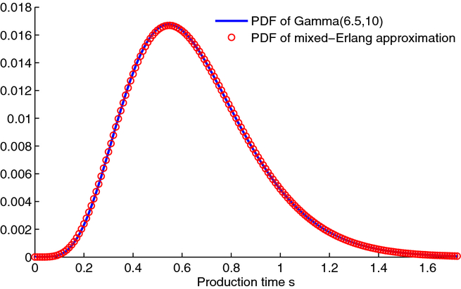
Probability Density Functions with Gamma Distribution and Its Mixed‐Erlang Approximation

Figure 2

Optimal Rationing Policies with Gamma Distribution and Its Mixed‐Erlang Approximation

Multiple Outstanding Orders: A Tandem MTS System

The preceding analysis relies on the assumption that there is at most one order outstanding at any point in time, i.e., no new order is issued if there is an order in the outstanding order pipeline. We relax this assumption in this section by considering a k‐stage serial inventory system, in which there may exist multiple outstanding orders at the same time. The stages are indexed by j = 0, 1, …, k − 1. The lowest stage storing the on‐hand inventory is represented by stage 0, stage j + 1 ships all its inventory to stage j, j = 0, 1, …, k − 2, and stage k − 1 places batch orders from an outside supplier with infinite supply.

We assume that the duration of each phase is exponentially distributed with a mean 1/μ, which implies that the production time of each order follows a k‐Erlang distribution with a mean k/μ. Due to the memoryless property of the exponential distribution, the orders placed at different times may pile up at some stage. To approximate the exogenous sequential supply system where the replenishment orders do not cross overtime (Zipkin 2000, § 7.4), we assume that all the orders in the same stage, once piled up together, will move simultaneously to the subsequent stage. In other words, an order may be delivered simultaneously with the other orders placed earlier. This is a common treatment in the literature (see, e.g., Johansen 2005, Kaplan 1970, Zipkin 2008).

Let (x, q ₁, …, q _k−1) denote the state of the system, where x is the on‐hand inventory level and q _i represents the size of the outstanding order at stage i, i = 1, …, k − 1. Note that x is a non‐negative integer and q _i is a non‐negative integer multiple of Q. Similar to the multi‐echelon inventory models (see, e.g., Pang et al. 2012), we can transform the state variable by a vector y = (y ₀,y ₁, …, y _k−1) such that y ₀ = x,

y_{i} = x + \sum_{j = 1}^{i} q_{j}, i = 1, \dots, k - 1

. Let

Y

be the corresponding state space and V(y) be the maximum value‐to‐go function. Uniformizing the underlying MDP with β = Λ + kμ and scaling the parameters such that γ + β = 1, the optimality equation can be expressed as

V (y) = T V (y),

(12)

where the operator T is defined on any real function

v : Y \to R

such that

\begin{matrix} T v (y) = - h x + \sum_{n = 1}^{N} λ_{n} T_{n} v (y) + μ \sum_{i = 1}^{k} H_{i} v (y), \\ T_{n} v (y) = max {p_{n} + v (y - e), - π_{n} + v (y)} 1_{{y_{0} > 0}} + [- π_{n} + v (y)] 1_{{y_{0} = 0}}, n = 1, \dots, N, \\ H_{1} v (y) = v (y_{1}, y_{1}, y_{2}, \dots, y_{k - 1}) - (y_{1} - y_{0}) C / Q, \\ H_{i} v (y) = v (y_{0}, y_{1}, \dots, y_{i - 2}, y_{i}, y_{i}, y_{i + 1}, \dots, y_{k - 1}), i = 2, \dots, k - 1, \\ H_{k} v (y) = max {v (y_{0}, y_{1}, \dots, y_{k - 2}, y_{k - 1} + Q), v (y_{0}, y_{1}, \dots, y_{k - 2}, y_{k - 1})} . \end{matrix}

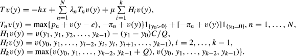
Here, the operators H _i addresses the order shipments from stage i to stage i − 1, i = 1, …, k − 1, and H _k addresses the ordering decisions at stage k − 1 (i.e., shipments from the outside supplier or stage k). For convenience, we define Δ_e V(y) = V(y) −V(y − e) and Δ_i V(y) = V(y) − V(y − Qe _i), where e _i is the k‐dimensional unit vector with the i‐th component being 1, i = 0, 1, …, k − 1, and

e = \sum_{i = 0}^{k - 1} e_{i}

Let s = (s ₁,⋯,s _k−1), where s _j = q ₁ + … + q _j represents the partial sum of the sizes of the outstanding orders (in batches) from stage 1 to stage j, j = 1,⋯,k − 1. Then, y = (x,x + s ₁,…,x + s _k−1). The following theorem characterizes the structure of the optimal policy.

Theorem 3

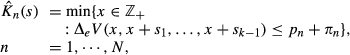
The optimal inventory replenishment policy is characterized by a state‐dependent reorder point:

\hat{R} (s) = min_{x} {Δ_{k - 1} V (x, x + s_{1}, \dots, x + s_{k - 1} + Q e_{k - 1}) \leq 0} - 1,

i.e., when the production status is s and the inventory level is below or at

\hat{R} (s)

, reorder a batch of size Q; otherwise, it is optimal not to place any order. In addition,

\hat{R} (s)

is increasing in s _i, i = 1, …, k − 2, and decreasing in s _k−1.

The optimal rationing control policy can be characterized by state‐dependent rationing threshold levels:

\begin{matrix} {\hat{K}}_{n} (s) & = min {x \in Z_{+} \\ : Δ_{e} V (x, x + s_{1}, \dots, x + s_{k - 1}) \leq p_{n} + π_{n}}, \\ n & = 1, \dots, N, \end{matrix}

such that for any s, if

x \geq {\hat{K}}_{n} (s)

, then accept the customer order of class n; otherwise, reject the customer order of class n. In addition,

{\hat{K}}_{n} (s)

is decreasing in s and n. In particular,

{\hat{K}}_{1} (s) = 0

This theorem characterizes the structure of the joint production and inventory rationing policy when there may be multiple orders outstanding at the same time. Note that compared with state y, y + Qe _k−1 has one more batch in the last stage and in the total number of outstanding orders. For i < k − 1, compared with y, y + Qe _i has one more batch in stage i, but has one less batch in stage i + 1, with the total number of outstanding orders being the same, which implies that in state y + Qe _i the outstanding orders are closer to their receivers. Part (a) shows that the optimal production control is characterized by a state‐dependent reorder point (in terms of inventory level). The optimal reorder point depends on the status of the production order pipeline, which is different from that derived under the assumption of at most one order outstanding where the optimal reorder point is independent of the delivery status. Note that given the total number of outstanding orders

s_{k - 1} = \sum_{l = 1}^{k - 1} q_{l}

(which implies that the system inventory position is x + s _k−1), an increase in q _i, i = 1, …, k − 2 implies that the (i + 1)‐th outstanding order is one phase closer to its receiver (while all else being equal). Then, the property that the reorder point

\hat{R} (s)

is increasing in s _i,i = 1, …, k − 2 implies that, given the same inventory position x + s _k−1, as the outstanding orders are closer to the final stage, it is more likely to place a new order. The property that

\hat{R} (s)

is decreasing in s _k−1 implies that, given the same inventory position x + s _k−1, as the inventory position increases, it is less likely to place a new order.

Part (b) shows that the optimal rationing policy can be characterized by the state‐dependent critical stock levels. The monotonicity of

{\hat{K}}_{n}

in n implies that the higher the inventory level is, the more the lower priority customer orders will be rejected. The monotonicity of

{\hat{K}}_{n}

in q implies that the more production orders are outstanding or the closer the outstanding orders are to the final stage, it is more likely to accept more customer orders.

We now translate the optimal policy structure back into the production status in terms of (i ₁, …, i _k−1). Let R(q ₁, …, q _k−1) and K _n(q ₁, …, q _k−1) be the respective production and inventory rationing control thresholds corresponding to

\hat{R} (q)

and

{\hat{K}}_{n} (q)

, respectively. The following corollary can be derived from Theorem 1.

Corollary 1

For 1 < l ≤ k − 1, if q _l−1 = q _l = 0, then the following inequalities hold:

R (q_{1}, \dots, q_{l - 1}, q_{l} + Q, \dots, q_{k - 1}) \leq R (q_{1}, \dots, q_{l - 1} + Q, q_{l}, \dots, q_{k - 1}) \leq R (q_{,} \dots, q_{l - 1}, q_{l}, \dots, q_{k - 1}),

(13)

K_{n} (q_{1}, \dots, q_{l - 1} + Q, q_{l}, \dots, q_{k - 1}) \leq K_{n} (q_{1}, \dots, q_{l - 1}, q_{l} + Q, \dots, q_{k - 1}) \leq K_{n} (q_{1}, \dots, q_{l - 1}, q_{l}, \dots, q_{k - 1}) .

(14)

Corollary 1 provides further insights into the optimal policy structure. From inequalities 13 we know that

\begin{matrix} R (q_{1}, \dots, q_{l - 1}, q_{l} + Q, \dots, q_{k - 1}) - \\ R (q_{1}, \dots, q_{l - 1}, q_{l}, \dots, q_{k - 1}) \\ \leq R (q_{1}, \dots, q_{l - 1} + Q, q_{l} \dots, q_{k - 1}) - \\ R (q_{1}, \dots, q_{l - 1}, q_{l}, \dots, q_{k - 1}) \leq 0 . \end{matrix}

These inequalities have the following implications. (1) The more orders are outstanding, the lower the reorder point is. (2) The effect of having one more batch that has completed k − l phases on the reorder point is stronger than the effect of having one more batch that has completed k − l + 1 phases. That is, the sensitivity of the reorder point to the number of outstanding orders in each phase decreases in the ages of the outstanding orders, where the age of an outstanding order refers to the number of phases it has completed. The reordering decision is most sensitive to the youngest outstanding orders that have completed only one phase.

From inequalities 14, we know that

\begin{matrix} K_{n} (q_{1}, \dots, q_{l - 1} + Q, q_{l}, \dots, q_{k - 1}) - K_{n} (q_{1}, q_{2}, \dots, q_{k - 1}) \\ \leq K_{n} (q_{1}, \dots, q_{l - 1}, q_{l} + Q, \dots, q_{k - 1}) \\ - K_{n} (q_{1}, q_{2}, \dots, q_{k - 1}) \leq 0, \end{matrix}

which implies that (a) the more orders are outstanding, the lower the rationing levels are (i.e., more customer orders will be accepted), but (b) the sensitivity of the rationing levels increases in the ages of the outstanding orders, which is different from the sensitivity of the reorder point.

The above monotone sensitivity is in line with the lost sales inventory models without the batch‐ordering restriction (see, e.g., Huh and Janakiraman 2010, Zipkin 2008) and the periodic‐review inventory‐pricing model (Pang et al. 2012). In the continuous‐review setting, Pang and Chen (2010) present some preliminary analysis for these properties when there are at most three orders outstanding (i.e., k = 3). However, it is not easy to further extend their analysis to the general case where k can be any positive integer. The state‐transformation approach enables us to analyze the structural properties in the context of the inventory rationing model with multiple outstanding orders.

The optimal policy parameters can be obtained by solving the optimality equation 12 using the conventional value iteration approach. Note that such an approach requires remembering the profit values for all the states. As the number of the outstanding orders increases, the state space increases exponentially and the number of iterations required before the algorithm converges may also increase significantly, and the computation effort becomes prohibitive. For more detailed discussions of the computational complexity and convergence of the value iteration algorithm, the reader may refer to Puterman (1994).

The following two examples demonstrate the structure of the optimal policies in a two‐phase and a three‐phase tandem MTS systems, respectively.

Example 2 Two‐Phase Tandem MTS System

Consider a system with a two‐phase Erlang production process (k = 2). The mean of each phase is 1/k (so that the mean of the total production time is 1). The other parameters are γ = 0.01, Q = 10, C = 10 + 5Q, h = 1, p = (10, 8, 5), π = (5, 2, 0), and λ = (5, 10, 30). The optimal reorder point and rationing levels are functions of the total size of the outstanding orders. As shown in Figure 3, both the reorder point and rationing levels are decreasing functions of the total size of the outstanding orders and the rationing levels are nested, which confirms the results of Corollary 1.

Figure 3

Structure of Optimal Policy (k = 2)

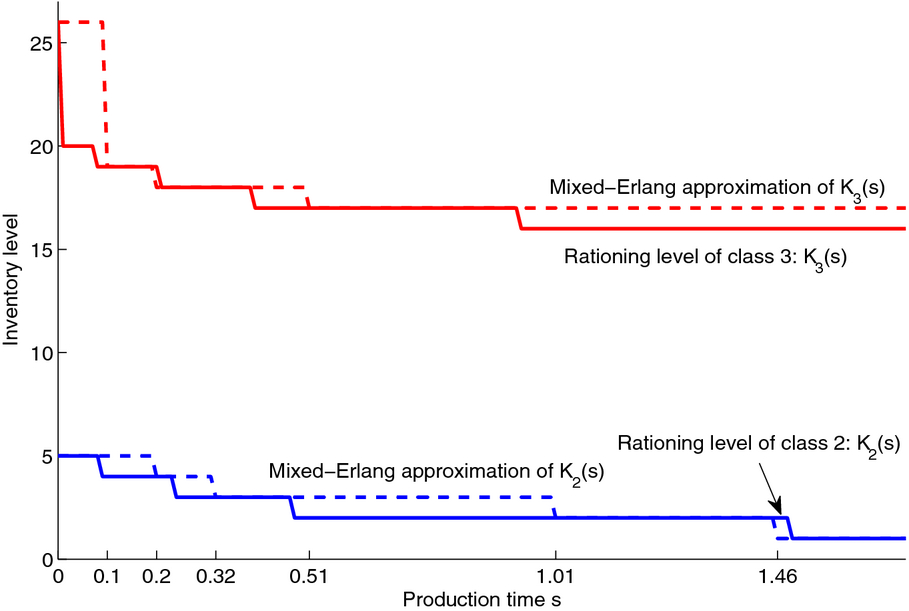
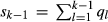
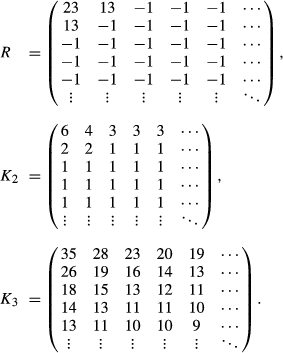
Example 3 Three‐Phase Tandem MTS System

Consider a system with a three‐phase Erlang production process (k = 3). The mean of each phase is 1/k (so that the mean of total production time is 1). The other parameters are the same as those in Example 2. The optimal reorder point and rationing levels are as follows.

\begin{matrix} R & = (\begin{matrix} 23 & 13 & - 1 & - 1 & - 1 & \dots \\ 13 & - 1 & - 1 & - 1 & - 1 & \dots \\ - 1 & - 1 & - 1 & - 1 & - 1 & \dots \\ - 1 & - 1 & - 1 & - 1 & - 1 & \dots \\ - 1 & - 1 & - 1 & - 1 & - 1 & \dots \\ ⋮ & ⋮ & ⋮ & ⋮ & ⋮ & ⋱ \end{matrix}), \\ K_{2} & = (\begin{matrix} 6 & 4 & 3 & 3 & 3 & \dots \\ 2 & 2 & 1 & 1 & 1 & \dots \\ 1 & 1 & 1 & 1 & 1 & \dots \\ 1 & 1 & 1 & 1 & 1 & \dots \\ 1 & 1 & 1 & 1 & 1 & \dots \\ ⋮ & ⋮ & ⋮ & ⋮ & ⋮ & ⋱ \end{matrix}), \\ K_{3} & = (\begin{matrix} 35 & 28 & 23 & 20 & 19 & \dots \\ 26 & 19 & 16 & 14 & 13 & \dots \\ 18 & 15 & 13 & 12 & 11 & \dots \\ 14 & 13 & 11 & 11 & 10 & \dots \\ 13 & 11 & 10 & 10 & 9 & \dots \\ ⋮ & ⋮ & ⋮ & ⋮ & ⋮ & ⋱ \end{matrix}) . \end{matrix}

Note that R and K _n are both decreasing in q _i, n = 2, 3, i = 1, 2. In particular, R(0,0) = 23 ≥ R(10,0) = R(0,10) = 13, …, and K ₂(0, 0) = 6 ≥ K ₂(10, 0) = 2 ≥ K ₂(0, 10) = 4, … It is clear that the above policy parameters satisfy inequalities 13 and 14.

Example 4 Performance Comparison.

It is interesting to know how sensitive the system performance is to the restriction on the number of outstanding orders. To this end, we solved a set of numerical examples to compare the performance of the system that allows at most one order outstanding with that of the system that allows multiple orders outstanding at any time. We examined the systems with two‐, three‐, and four‐phase Erlang production times, respectively. The average production time is 1 and the mean time per phase is 1/k. For ease of comparison, we use the long‐run average profit as the performance measure.

The system parameters are still γ = 0.01, Q = 10, C = 10 + 5Q, h = 1, p = (10, 8, 5), π = (5, 2, 0), and λ = (5, 10, 30). Let δ _m be the average profit of the system with m‐phase production times, m = 2, 3, 4. We varied Q to examine the effect of batch size. Table 1 reports the results. The first column is the batch size, columns 2–4 record the average profits (

δ_{2}^{O}

) when there is at most one order outstanding, the average profit (

δ_{2}^{M}

) when there are multiple orders outstanding, and the percentage profit increments by allowing multiple outstanding orders

(Δ_{2} = \frac{δ_{2}^{M} - δ_{2}^{O}}{δ_{2}^{O}} \times 100 %)

, respectively. Similarly, columns 5–7 and columns 8–10 correspond to the models with 3 and 4 phases. Table 2 reports the optimal policies of the models with 2 and 3 phases. Note that for the tandem systems, we only report the cases when the systems have at most only one order outstanding. We have the following observations.

Table 1

Performances: One Outstanding Order vs. Multiple Outstanding Orders

	k = 2			k = 3			k = 4
Size	One	Multiple	Percentage increments	One	Multiple	Percentage increments	One	Multiple	Percentage increments
Q	$δ_{2}^{O}$	$δ_{2}^{M}$	Δ₂ (%)	$δ_{3}^{O}$	$δ_{3}^{M}$	Δ₃ (%)	$δ_{4}^{O}$	$δ_{4}^{M}$	Δ₄ (%)
10	8.21	14.37	74.95	9.86	17.77	80.19	10.73	19.62	82.82
11	11.27	14.87	40.74	13.27	19.06	43.63	14.39	20.82	44.69
12	13.77	17.05	23.84	16.04	20.03	24.88	17.38	21.72	24.95
13	15.70	17.96	14.37	18.22	20.80	14.15	19.70	22.45	14.00
14	17.23	18.69	8.51	19.85	21.41	7.82	21.43	23.06	7.58
15	18.41	19.27	4.67	21.06	21.91	4.07	22.70	23.57	3.84
20	21.26	21.25	−0.04	23.76	23.74	−0.06	25.24	25.24	−0.00
25	21.97	21.99	0.07	24.25	24.26	0.05	25.61	25.62	0.03
30	22.03	22.05	0.08	24.10	24.14	0.19	25.34	25.39	0.18
35	21.69	21.71	0.12	23.64	23.69	0.22	24.93	24.89	−0.15
40	21.14	21.18	0.17	23.07	23.10	0.13	24.27	24.21	−0.22

Table 2

Optimal Policies: One Outstanding Order vs. Multiple Outstanding Orders

Size	One outstanding order		Multiple outstanding orders
k = 2
Q	R	$(\begin{matrix} K_{2} (0) & K_{2} (1) \\ K_{3} (0) & K_{3} (1) \end{matrix})$	(R ₀, R ₁)	$(\begin{matrix} K_{2} (0) & K_{2} (1) \\ K_{3} (0) & K_{3} (1) \end{matrix})$
10	31	$(\begin{matrix} 7 & 4 \\ 46 & 38 \end{matrix})$	(25, 15)	$(\begin{matrix} 6 & 3 \\ 40 & 31 \end{matrix})$
15	24	$(\begin{matrix} 5 & 2 \\ 36 & 25 \end{matrix})$	(23, 6)	$(\begin{matrix} 5 & 2 \\ 35 & 24 \end{matrix})$
20	21	$(\begin{matrix} 5 & 2 \\ 33 & 21 \end{matrix})$	(21, −1)	$(\begin{matrix} 5 & 2 \\ 33 & 21 \end{matrix})$
25	20	$(\begin{matrix} 4 & 2 \\ 33 & 19 \end{matrix})$	(20, −1)	$(\begin{matrix} 4 & 2 \\ 33 & 19 \end{matrix})$
30	19	$(\begin{matrix} 4 & 1 \\ 32 & 18 \end{matrix})$	(19, −1)	$(\begin{matrix} 4 & 1 \\ 32 & 18 \end{matrix})$
35	18	$(\begin{matrix} 4 & 1 \\ 33 & 17 \end{matrix})$	(18, −1)	$(\begin{matrix} 4 & 1 \\ 33 & 17 \end{matrix})$
40	18	$(\begin{matrix} 4 & 1 \\ 33 & 16 \end{matrix})$	(18, −1)	$(\begin{matrix} 4 & 1 \\ 33 & 16 \end{matrix})$
k = 3
Q	R	$(\begin{matrix} K_{2} (0) & K_{2} (1) & K_{2} (2) \\ K_{3} (0) & K_{3} (1) & K_{3} (2) \end{matrix})$	(R(0, 0), R(1, 0), R(0,1))	$(\begin{matrix} K_{2} (0, 0) & K_{2} (0, 1) & K_{2} (1, 0) \\ K_{3} (0, 0) & K_{3} (0, 1) & K_{3} (1, 0) \end{matrix})$
10	31	$(\begin{matrix} 7 & 5 & 3 \\ 45 & 37 & 35 \end{matrix})$	(24, 14, 13)	$(\begin{matrix} 6 & 4 & 2 \\ 37 & 29 & 27 \end{matrix})$
15	23	$(\begin{matrix} 6 & 4 & 2 \\ 33 & 25 & 21 \end{matrix})$	(22, 6, 3)	$(\begin{matrix} 5 & 3 & 1 \\ 33 & 24 & 20 \end{matrix})$
20	21	$(\begin{matrix} 5 & 3 & 1 \\ 31 & 21 & 16 \end{matrix})$	(21, −1, −1)	$(\begin{matrix} 5 & 3 & 1 \\ 31 & 21 & 16 \end{matrix})$
25	20	$(\begin{matrix} 5 & 3 & 1 \\ 30 & 20 & 15 \end{matrix})$	(20, −1, −1)	$(\begin{matrix} 5 & 3 & 1 \\ 30 & 20 & 15 \end{matrix})$
30	19	$(\begin{matrix} 5 & 3 & 1 \\ 30 & 20 & 14 \end{matrix})$	(19, −1, −1)	$(\begin{matrix} 5 & 3 & 1 \\ 30 & 20 & 14 \end{matrix})$
35	19	$(\begin{matrix} 5 & 3 & 1 \\ 31 & 19 & 13 \end{matrix})$	(19, −1, −1)	$(\begin{matrix} 5 & 3 & 1 \\ 30 & 19 & 13 \end{matrix})$
40	18	$(\begin{matrix} 5 & 3 & 1 \\ 31 & 19 & 12 \end{matrix})$	(18, −1, −1)	$(\begin{matrix} 5 & 3 & 1 \\ 31 & 19 & 12 \end{matrix})$

First, for all k, as the batch size Q increases, the optimal reorder point, rationing levels, and profit difference tend to decrease. This fits the intuition that the larger the order size is, the less frequently the replenishment order is placed and more demand orders are accepted. When Q is small, the reorder point tends to be greater than Q, R > Q, and the profit difference is significant, which implies that the single‐outstanding‐order assumption may lead to a greater loss. When Q is large, the reorder point tends to be smaller than Q, R < Q, and the profit difference becomes close to zero, which implies that it may suffice to allow at most one outstanding order.

Second, comparing the single‐outstanding‐order system and tandem system, it is interesting to observe that given the same production status, especially when the batch size is small, the tandem system tends to have lower rationing levels and reorder points. This may be due to the opportunity to have multiple outstanding orders before the current order is delivered and then the tandem system will be more likely to have higher inventory levels later. The anticipation of having more inventory induces the manager to set lower rationing levels to accept more orders and lower the reorder point to avoid the inventory over‐stocking risk. However, when the batch size is large and thus R < Q, the tandem system only allows at most one order outstanding and the rationing levels are effectively the same as those of the system with at most one order outstanding. This finding confirms the view that when the batch size is sufficiently large, the system with at most one outstanding order provides a good approximation of the tandem system.

Concluding Remarks

This study addresses the inventory rationing problem for a lost sales MTS system with batch ordering and multiple demand classes. We first consider the case with general production times and a single outstanding order and then approximate the production time distribution by the phase‐type distributions. To address the cases with multiple outstanding orders, we consider a MTS tandem system. We introduce a transformation approach that enables us to characterize the structure of the optimal policy and obtain some new structural results. These results provide some new insights into the inventory rationing problems.

Nevertheless, our model is restricted to the assumptions of Poisson demand and fixed batch size. In addition, although we are able to characterize the structure of the optimal policies when there are multiple outstanding orders, it is still unrealistic to compute the optimal policies directly due to the curse of dimensionality. An important future research direction is to use some of the insights provided by the structural analysis to design effective optimal or heuristic algorithms.

More importantly, we have a limited understanding on backlog systems with batch production/ordering. Huh and Janakiraman (2010) show that the (R,nQ) policy is optimal when there is only a single demand class. In the presence of multiple demand classes, the questions as to whether the (R,nQ) policy is still optimal and whether the optimal rationing control is still of threshold type remain open. We aim to address these issues in future research.

Footnotes

Acknowledgments

We sincerely thank Professor Panos Kouvelis (the department editor), the senior editor, and three anonymous referees for their valuable comments and suggestions that helped improve this study. The corresponding author, Houcai Shen, was partly supported by National Natural Science Foundation of China (No. 71071074) and MOE (Ministry of Education in China) Project (No 20120091110059).

References

Arslan

Graves

S. C.

Roemer

. 2007. A single‐product inventory model for multiple demand classes. Oper. Res. 53(9): 1486–1500.

Benjaafar

ElHafsi

. 2006. Production and inventory control of a single product assemble‐to‐order system with multiple customer classes. Manage. Sci. 52: 1896–1912.

Berk

Gürler

Ü.

. 2008. Analysis of the (Q,r) inventory model for perishables with positive lead times and lost sales. Oper. Res. 56(5): 1238–1246.

Buchanan

D. J.

Love

R. F.

. 1985. A (Q,R) inventory model with lost sales and erlang‐distributed leadtimes. Nav. Res. Log. Q. 32(4): 605–611.

Chen

2000. Optimal policies for multi‐echelon inventory problems with batch ordering. Oper. Res. 48:376–389.

Chen

Simchi‐Levi

. 2012. Pricing and inventory management. Philips

and Özalp

Ö.

, eds. Handbook of Pricing. Oxford University Press, United Kingdom, 784–822.

Chen

Feng

. 2006. Joint Management of finished goods inventory and demand process for a make‐to‐stock product: A computational approach. IEEE Trans. Automat. Contr. 51(2): 258–273.

Chen

Feng

. 2009. Coordinating batch production and pricing of a make‐to‐stock product. IEEE Trans. Automat. Contr. 54(7): 1674–1680.

Cheng

T. C. E.

Gao

C. Y.

Shen

H. C.

. 2011. Production and inventory rationing in a make‐to‐stock system with a failure‐prone machine and lost sales. IEEE Trans. Automat. Contr. 56(5): 1176–1180.

10.

Cohen

M. A.

Kleindorfer

P. R.

Lee

H. L.

. 1988. Service constrained (s,S) inventory systems with priority demand classes and lost sales. Manage. Sci. 34(4): 482–499.

11.

Deshpande

Cohen

M. A.

Donohue

. 2003. A threshold inventory rationing policy for service‐differentiated demand classes. Manage. Sci. 49(6): 683–703.

12.

Ding

Kouvelis

Milner

J. M.

. 2006. Dynamic pricing through discounts for optimizing multi‐class demand fulfillment. Oper. Res. 54(1): 169–183.

13.

Elmaghraby

Keskinocak

. 2003. Dynamic pricing in the presence of inventory considerations: Research overview, current practices, and future directions. Manage. Sci. 49(10): 1287–1309.

14.

Fadiloglu

M. M.

Bulut

Ö.

. 2010. A dynamic rationing policy for continuous‐review inventory systems. European. J. Oper. Res. 202(3): 675–685.

15.

A.Y.

1997. Inventory rationing in a make‐to‐stock production system with several demand classes and lost sales. Manage. Sci. 43(8): 1093–1103.

16.

A.Y.

2000. Stock rationing in an M/E _k/1 make‐to‐stock queue. Oper. Res. 46(1): 77–87.

17.

Hadley

Whitin

T. M.

. 1963. Analysis of Inventory Systems. Prentice‐Hall, Englewood Cliffs, NJ.

18.

Hill

R. M.

Johansen

S. G.

. 2004. Optimal and near‐optimal policies for lost sales inventory models with at most one replenishment order outstanding. Eur. J. Oper. Res. 169(1): 111–132.

19.

Huh

Janakiraman

. 2010. On the optimal policy structure in serial inventory systems with lost sales. Oper. Res. 58(2): 481–491.

20.

Huh

Janakiraman

. 2012. On optimal policies for inventory systems with batch ordering. Oper. Res. 60(4): 797–802.

21.

Johansen

S. G.

2005. Base‐stock policies for the lost sales inventory system with Poisson demand and Erlang lead times. Int. J. Prod. Econ. 93: 429–437.

22.

Johansen

S. G.

Thorstenson

. 2004. The (r,q) policy for the lost‐sales inventory system when more than one order may be outstanding. Working Paper, University of Aarhus , Denmark.

23.

Kaplan

1970. A dynamic inventory model with stochastic lead times. Manage. Sci. 16: 491–507.

24.

Kimes

S. E.

1989. Yield management: A tool for capacity constrained service firms. J. Oper. Manag. 8: 348–363.

25.

Kleijn

M. J.

Dekker

. 1999. An overview of inventory systems with several demand classes. Lect. Notes Econ. Math. 480: 253–265.

26.

McWilliams

2001. Lean machine: How Dell fine‐tunes its PC pricing to gain edge in slow market, Wall St. J. (June 8), p. A1.

27.

Melchiors

2001. Rationing policies for an inventory model with several demand classes and stochastic lead times. Working Paper, Department of Operations Research, University of Aarhus , Denmark.

28.

Melchiors

Dekker

Kleijn

M. J.

. 2000. Inventory rationing in an (s,Q) inventory model with lost sales and two demand classes. J. Oper. Res. Soc. 51(1): 111–122.

29.

Möllering

Thonemann

U. W.

. 2008. An optimal critical level policy for inventory systems with two demand classes. Nav. Res. Log. 55(7): 632–642.

30.

Nahmias

Demmy

W. S.

. 1981. Operating characteristics of an inventory system with rationing. Manage. Sci. 27(11): 1236–1245.

31.

Pang

Chen

F. Y.

. 2010. Dynamic inventory‐pricing control of a continuous review system with batch ordering and random leadtimes. Working Paper, Lancaster University , Lancaster.

32.

Pang

Chen

F. Y.

Feng

. 2012. A note on the structure of joint inventory‐pricing control with leadtimes. Oper. Res. 60(3): 581–587.

33.

Porteus

E. L.

2002. Foundations of Stochastic. Inventory Theory, Stanford University Press, Stanford, CA.

34.

Puterman

1994. Markov Decision Process: Discrete Stochastic Dynamic Programming. John Wiley and Sons, New York.

35.

Song

J. S.

2000. A note on assemble‐to‐order system with batch ordering. Manage. Sci. 46(5): 739–743.

36.

Talluri

van Ryzin

. 2004. The Theory and Practice of Revenue Management. Kluwer Academic Publishers, New York.

37.

Tijms

H. C.

1994. Stochastic Models: An Algorithmic Approach. John Wiley and Sons, New York.

38.

Veinott

A. F.

1965. Optimal policy in a dynamic, single product, nonstationary inventory model with several demand classes. Oper. Res. 13(5): 761–778.

39.

Zipkin

1986. Stochastic lead‐times in continuous time inventory models. Nav. Res. Log. 33: 763–774.

40.

Zipkin

1988. The use of phase‐type distributions in inventory control models. Nav. Res. Log. 35(2): 247–257.

41.

Zipkin

2000. Foundations of Inventory Management. McGraw‐Hill, Boston.

42.

Zipkin

2008. On the structure of lost‐sales inventory models. Oper. Res. 56(4): 937–944.