Benefits of Hybrid Lateral Transshipments in Multi‐Item Inventory Systems under Periodic Replenishment

Abstract

Lateral transshipments are a method of responding to shortages of stock in a network of inventory‐holding locations. Conventional reactive approaches only seek to meet immediate shortages. The study proposes hybrid transshipments which exploit economies of scale by moving additional stock between locations to prevent future shortages in addition to meeting immediate ones. The setting considered is motivated by retailers who operate networks of outlets supplying car parts via a system of periodic replenishment. It is novel in allowing non‐stationary stochastic demand and general patterns of dependence between multiple item types. The generality of our work makes it widely applicable. We develop an easy‐to‐compute quasi‐myopic heuristic for determining how hybrid transshipments should be made. We obtain simple characterizations of the heuristic and demonstrate its strong cost performance in both small and large networks in an extensive numerical study.

Keywords

inventory control multi‐item lateral transshipments dynamic programming

Introduction

Increased information in modern inventory networks offers managers the opportunity to pool risk through cooperation between replenishment points. Lateral transshipments are stock movements between locations in the same echelon of an inventory system. This transportation of goods can be used to rebalance stock proactively across the system or to meet shortages reactively as they occur.

When a reactive transshipment is triggered, conventional policies only meet the immediate shortfall. Stock is moved from a location with a surplus to the one experiencing the shortage. However, in many practical scenarios a large proportion of the associated vehicle, fuel and labor costs are independent of the amount transshipped. In such cases conventional reactive approaches ignore the economies of scale and the risk of future shortages which may make it beneficial to transship more than is required to meet the immediate shortfall. Proactive approaches to transshipment have conventionally rebalanced stock through the logistically complex and costly device of reallocating the entire network's inventory at isolated time points. The hybrid approach proposed here exploits the above potential for cost savings by rebalancing stock between pairs of locations when a shortage occurs at one of them. It thus has the same triggering mechanism as conventional reactive transshipments and minimal additional implementation overhead.

A scenario of particular interest to this study is the sale of car parts including tyres and exhaust systems from networks of depots which typically fit new parts and conduct repairs. Common features of such networks include the following: stock for replenishment is from a central store from which large trucks conduct tours to resupply parts of the network. The determination of such tours is outside of the scope of this work and we shall suppose that the periodicity of each location's replenishment is fixed. Depots are often in centers of population where rents are high and space for inventory is limited. This may force inventory levels lower than an (unconstrained) economic analysis might indicate and will fuel the need for the pooling of stock. Demand for items is likely non‐stationary as well as stochastic. For example, the demand pattern at weekends may well be different from that during the working week. Further, individual customers are unlikely to require a single item. Individual demands will typically be for one or more of each of several item types.

The model considered in the study assumes the periodic review and replenishment of stock. It develops the reactive transshipment model of Archibald et al. (2010) in a way which captures the features mentioned in the preceding paragraph. It is novel in the literature in the generality of its characterization of demand. Demand instances are assumed to occur in a non‐stationary manner, while individual customer requirements (how many of each item type) are drawn from a general joint distribution. This is a huge advance over the customary assumption of a stationary Poisson process of singleton demands for one item type only. Hence the work not only delivers significant cost savings over current proposals but is also relevant to a wider range of practical scenarios.

Following a review of the existing literature in section 2, a detailed description of the model is given in section 3. Section 4 is the analytical heart of the study and is where the hybrid transshipment heuristic is developed. Key contributions include a characterization of policy structure, analytical insight into the setting of replenishment levels and the development of an easily computed numerical lower bound for the cost rate achievable in some cases where locations are replenished simultaneously. Section 5 contains an account of an extensive numerical study designed to evaluate the performance of the new policy. Results elucidate the considerable performance gain achieved over existing approaches and suggest that the hybrid proposal closes a large part of the suboptimality gap left by them.

Literature

Research on transshipments in inventory networks has primarily focussed on their use in the context of stationary demand for a single item type. The broad approach taken to transshipping has been reactive, proactive, or a hybrid of the two. We now consider these approaches in turn.

Much of the literature on reactive transshipments assumes periodic replenishment. Krishnan and Rao (1965) assume demand is met at the end of each review period, so transshipments can be arranged after all demand for the period has been observed. Taking a similar approach to the modeling of demand, Robinson (1990) shows that an order‐up‐to policy is optimal while Lien et al. (2011) explore optimal network configurations. In many situations customers require, or at least value, immediate service. An assumption that demand for a period can be observed before transshipments are planned is plainly not always appropriate. Archibald et al. (1997) allow multiple transshipments in each review period. A location makes a transshipment request whenever a shortage occurs, but transshipment requests are not always met (a situation known as partial pooling). The form of an optimal replenishment and transshipment policy is established for networks with two locations. Çömez et al. (2012) characterize an optimal transshipment policy for two locations in a similar setting with positive replenishment and transshipment lead times. Archibald (2007) and Archibald et al. (2010) also consider reactive transshipments whenever a shortage occurs, but develop heuristic policies that can be applied to networks of any size. The current work extends the latter inter alia by introducing a proactive element into the transshipment policies considered and through its much more general setting of non‐stationary demand for many item types.

Other inventory problems related to reactive approaches arise in a multi‐product setting where substitution with products of higher specification (Rao et al. 2004, Xu et al. 2011) and allocation of stocks of unfinished products (Swaminathan and Tayur 1998) or common components (Gerchak and Henig 1986) serve a similar purpose to transshipments. However, products in this stream of work correspond to our locations and so when these problems are viewed as transshipment problems they concern single items only and are hence less general than our multiple item scenarios. These problems also contrast with ours in offering no incentive for proactive action and decisions about which items to “transship” and in what quantity are purely reactive.

Research on proactive transshipment focuses predominantly on periodic replenishment. It is possible to think of proactive transshipments as including an element of reactive transshipment in the sense that they aim to rebalance inventory to best satisfy existing shortages and future demand (Lee et al. 2007). However in most cases, transshipment is only allowed at fixed points in each review period (Gross 1963, Lee et al. 2007). The approach of Agrawal et al. (2004) is closest in spirit to the current work as the timings of transshipments are determined dynamically. However, in contrast to the current work, only one proactive transshipment is allowed per period and inventory is redistributed across all locations. These studies all demonstrate some benefit from stock rebalancing which purely reactive approaches do not exploit.

Reactive and proactive transshipments have also been considered in the context of continuous review replenishment, but this is of less relevance to the current work which focuses on periodic review. For a more detailed review of the literature, the reader is referred to Paterson et al. (2010).

Zhao et al. (2008) consider reactive and proactive transshipments together. Their production based model uses a conventional reactive transshipment when shortages occur but also separately allocates new stock when it is produced. To the authors' knowledge, hybrid transshipments of the type considered in this study have previously only been considered by Paterson et al. (2012). That study develops heuristics for continuous replenishment review under compound Poisson demand for a single item. The methods used are very different from those in the current work.

We are unaware of any contributions in the literature which match the generality of our modeling of demand. Few consider either non‐stationary demand or many item types. Herer and Tzur (2001, 2003) do consider time‐varying demand but it is deterministic. Hence they can plan for known future demand in a manner which is not possible in a stochastic setting. In Archibald et al. (1997), replenishment decisions for many item types are linked via a storage space constraint while in Wong et al. (2005) and Kranenburg and van Houtum (2009) there is a linking constraint on average service time. Our stochastic non‐stationary model for multi‐item demand is a huge advance in generality on previous work and has great relevance for applications.

Inventory System Model

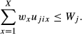
We consider a network with N locations, each of which carries an inventory of X distinct item types. Locations are replenished periodically from a central depot. The review period for location i is T _i and hence all item types at i are replenished at times

t_{i}^{*} + n T_{i}, n \in N

, where

t_{i}^{*} \in [0, T_{i}]

is the time of the first replenishment at i after 0. For reasons given in the Introduction, the replenishment periods T _i, 1 ≤ i ≤ N, will be taken as given and fixed throughout the study. Distinct locations across the network may have different review periods and so locations are not assumed to replenish simultaneously. We deploy the notation t _i(t) for the time from some arbitrary

t \in R^{+}

until the next replenishment at i. Should a replenishment epoch for location i occur at some time

t_{i}^{*} + n T_{i}

, the inventory of each item type x is restored to the level

S_{i x} (t_{i}^{*} + n T_{i})

. The dependence of the replenishment levels upon the time at which replenishment occurs can be exploited in cases where the non‐stationarity of the demand is very strong. See section 4.3 for further comments on the determination of the order‐up‐to levels

S_{i x} (t_{i}^{*} + n T_{i}), n \in N

. Until then, we shall regard them as fixed. Due to the dependence of the replenishment levels on time, it is theoretically possible for the inventory level of an item at a replenishment epoch to exceed the intended replenishment level. For the purposes of the model we develop, it is assumed that any excess inventory at a location is removed during “replenishment”. In practice, this situation would be extremely rare and so this assumption will not have a significant impact on the performance of the heuristics developed.

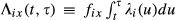
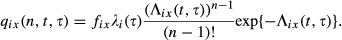
Customers arrive at location i according to a non‐homogeneous Poisson process independently of arrivals at other locations, with rate at time t given by λ _i(t). We assume that successive demands at location i are independent and identically distributed. We shall use D _i ≡ (D _i1, D _i2,…, D _iX) for the random X‐vector denoting a single customer demand at location i, with D _ix denoting the size of a single customer's demand for item type x. Plainly

P (\sum_{x = 1}^{X} D_{i x} \geq 1) = 1

. We shall use the notation f _{i
d} ≡ P(D _i = d) for the multivariate probability mass function (pmf) for location i demands and write

f_{i x} \equiv P (D_{i x} \geq 1) = \sum_{{d : d_{x} \geq 1}} f_{i d}

(1)

for the probability that a single customer at location i demands at least one item of type x. If such a demand occurs, we refer to the customer as an x‐customer. A customer may be an x‐customer for several distinct x. The pmf for the size of demands for item type x from x‐customers is denoted by

f_{i x d} \equiv P (D_{i x} = d | D_{i x} \geq 1) = \frac{\sum_{{d : d_{x} = d}} f_{i d}}{f_{i x}} .

(2)

The above implies that x‐customers arrive at location i according to a non‐homogeneous Poisson process whose rate at time t is f _ix λ _i(t) with the size of x‐demand from individual x‐customers determined by the pmf {f _ixd, d ≥ 1}, the latter having finite mean and variance μ _ix and

σ_{i x}^{2}

respectively. Additionally, we use

f_{i x d}^{n}

for the derived probability that n x‐customers together demand exactly d of item type x at location i.

A consequence of allowing composite multivariate demand is that shortages may be of more than one piece of inventory and/or of multiple item types. However, in the description of our methodology in the next section, we shall assume that transshipments come from a single location. This common constraint derives principally from practice as coordinating movements from more than one location can considerably complicate operating the policy. Further, we shall allow transshipments which meet only part of a current shortage. However, an indication will be given in section 4 of how our methodology may be extended to allow transshipments of a more complex structure and/or meet an “all or nothing” demand requirement.

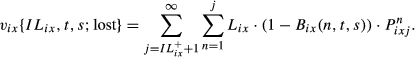
Several costs are involved in the operation of an inventory network and most influence the potential benefit of transshipment. The only cost assumed exogenous is the initial cost to purchase a piece of inventory. Holding costs are incurred at location i for items of type x at a rate h _ix per unit of stock and per unit of time. Further, penalty costs are incurred whenever demand cannot be met immediately. Two methods of penalizing unmet demand are considered. A one‐off cost of L _ix per unit of unmet demand of item type x is incurred if it is lost from the system. 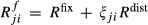Alternatively, the demand can be backordered with a penalty cost b _ix which is incurred per unit of item type x and per unit of time the item remains out of stock. We are able to address both cost structures. Finally, the cost associated with each transshipment from location j to location i has two elements: a fixed cost per transshipment

R_{j i}^{f}

, and a cost per unit of item type x transshipped,

R_{j i x}^{u}

Development and Analysis of the Hybrid Transshipment Heuristic

To develop a heuristic for transshipment decisions (from where and how much), we broadly follow Axsäter (2003) and Paterson et al. (2012) in their espousal of a quasi‐myopic approach to an otherwise intractable problem. Under this approach, all decisions are taken in the light of an assumed future for the system which has no transshipments. Expressed technically, the dynamic transshipment policy produced is obtained by performing a single dynamic programming policy improvement step from a no transshipment policy.

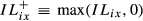
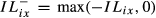
We proceed to give computations of the expected costs incurred under an assumption that no future transshipments are made. In what follows, we use IL _ix for the inventory level of item type x at location i at some arbitrary time

t \in R^{+}

(deemed the current epoch) and t + s, s ≤ t _i(t) for some future time no later than location i's next replenishment. We write IL _i ≡ (IL _i1,IL _i2,…,IL _iX) for the vector of inventory levels of all item types at i and denote by v _i{IL _i, t, s} the expected inventory costs incurred at location i during the time interval (t, t + s).

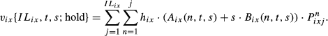
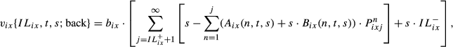
Before continuing we note that, notwithstanding the fact that demands across distinct item types may well be correlated, the expectation operator is linear so we can give an additive decomposition of total costs at location i which give contributions from individual item types. Hence,

\begin{matrix} v_{i} {{IL}_{i}, t, s} & = \sum_{x = 1}^{X} v_{i x} {I L_{i x}, t, s} = \sum_{x = 1}^{X} (v_{i x} \{I L_{i x}, t, s; hold\} \\ + v_{i x} \{I L_{i x}, t, s; lost\} + v_{i x} \{I L_{i x}, t, s; back\}), \end{matrix}

(3)

where Equation 3 expresses a decomposition of the total costs per item type into costs due to the holding of inventory (first term on the rhs of Equation 3) and costs associated with not being able to meet demand (second and third terms). In practice we either have L _ix > 0, b _ix = 0 ∀ i,x (lost sales model) or L _ix = 0, b _ix > 0 ∀i,x (backordered sales model). Please note that if b _ix > 0 any inventory level IL _ix may be negative, this corresponding to a number of currently backordered items; we use

I L_{i x}^{+} \equiv max (I L_{i x}, 0)

and

I L_{i x}^{-} = max (- I L_{i x}, 0)

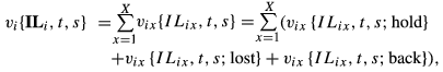
To compute v _ix{IL _ix,t,s;hold}, we further disaggregate into a sum with a contribution from each of the IL _ix units of stock of type x present at location i at time t, considered in the order in which they are demanded. If κ _ijx is the holding cost of the jth unit of type x stock at i and

E (κ_{i j x}^{n})

is its conditional expectation when the jth unit of type x stock is demanded by the nth x‐customer at i, then

v_{i x} {I L_{i x}, t, s; hold} = \sum_{j = 1}^{I L_{i x}} E (κ_{i j x}) = \sum_{j = 1}^{I L_{i x}} \sum_{n = 1}^{j} E (κ_{i j x}^{n}) \cdot P_{i x j}^{n},

(4)

where we use

P_{i x j}^{n}

for the probability that the jth unit of type x inventory is demanded by the nth x‐customer at location i after time t. Please note that the quantities

P_{i x j}^{n}

may be easily recovered from the quantities

f_{i x d}^{m}

defined in section 3. Now choose a time τ ∈ (t, t + s). The number of x‐customers arriving at location i during the interval (t, τ) has a Poisson distribution with mean

Λ_{i x} (t, τ) \equiv f_{i x} \int_{t}^{τ} λ_{i} (u) d u

. It follows that the probability that the nth x‐customer after t arrives during the interval (τ,τ + δτ) has the form q _ix(n, t, τ)δτ + o(δτ) where

q_{i x} (n, t, τ) = f_{i x} λ_{i} (τ) \frac{{(Λ_{i x} (t, τ))}^{n - 1}}{(n - 1)!} exp {- Λ_{i x} (t, τ)} .

(5)

By conditioning on the time at which the nth customer after t arrives we deduce that

E (κ_{i j x}^{n}) = h_{i x} \cdot (A_{i x} (n, t, s) + s \cdot B_{i x} (n, t, s)),

(6)

where A _ix(n, t, s) and B _ix(n, t, s) are given by

A_{i x} (n, t, s) = \int_{t}^{t + s} (τ - t) \cdot q_{i x} (n, t, τ) d τ

(7)

and

B_{i x} (n, t, s) = 1 - \int_{t}^{t + s} q_{i x} (n, t, τ) d τ = \sum_{m = 0}^{n - 1} \frac{{(Λ_{i x} (t, t + s))}^{m}}{m!} exp {- Λ_{i x} (t, t + s)} .

(8)

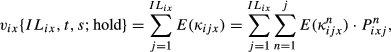
Substituting into Equation 4 we now have that

v_{i x} {I L_{i x}, t, s; hold} = \sum_{j = 1}^{I L_{i x}} \sum_{n = 1}^{j} h_{i x} \cdot (A_{i x} (n, t, s) + s \cdot B_{i x} (n, t, s)) \cdot P_{i x j}^{n} .

(9)

A similar analysis yields that expected costs from lost sales are given by

v_{i x} {I L_{i x}, t, s; lost} = \sum_{j = I L_{i x}^{+} + 1}^{\infty} \sum_{n = 1}^{j} L_{i x} \cdot (1 - B_{i x} (n, t, s)) \cdot P_{i x j}^{n} .

(10)

Write D _ix(t, s) for the demand for x‐items at location i between times t and t + s. It is straightforward to show that the expression in Equation 10 may alternatively be expressed as

\sum_{j = I L_{i x}^{+} + 1}^{\infty} L_{i x} \cdot P (D_{i x} (t, s) \geq j),

(11)

which may be well approximated by a corresponding finite sum

\sum_{j = I L_{i x}^{+} + 1}^{M_{i x} (t, s)}

where M _ix(t, s) is chosen to make P(D _ix(t, s) ≥ M _ix(t, s)) sufficiently small. In practice we choose

\begin{matrix} M_{i x} (t, s) = E (D_{i x} (t, s)) + 3 \sqrt{var (D_{i x} (t, s))} \\ = μ_{i x} \cdot Λ_{i x} (t, t + s) + 3 \sqrt{(μ_{i x}^{2} + σ_{i x}^{2}) \cdot Λ_{i x} (t, t + s)} . \end{matrix}

(12)

For the backorder costs a similar argument to that involving the above calculation of holding costs is needed to compute v _ix{IL _ix, t, s;back}. Each unit of potential excess x‐demand incurs a backorder cost over the period between the corresponding x‐customer arrival time and t + s. Further, x‐items already on backorder at t incur backorder costs over the entire period. This gives

v_{i x} {I L_{i x}, t, s; back} = b_{i x} \cdot [\sum_{j = I L_{i x}^{+} + 1}^{\infty} [s - \sum_{n = 1}^{j} (A_{i x} (n, t, s) + s \cdot B_{i x} (n, t, s)) \cdot P_{i x j}^{n}] + s \cdot I L_{i x}^{-}],

(13)

which may also be well approximated by a finite sum. We can now use Equations 9, (10), and 13 to obtain the key quantity v _i{IL _i,t,s} from Equation 3.

Development of the Hybrid Heuristic Via DP Policy Improvement

We consider a scenario in which the system has inventory levels {(IL _jx), 1 ≤ x ≤ X, 1 ≤ j ≤ N} at some time

t \in R^{+}

when a demand d _i which cannot be fully met from local stock arises at location i. Hence d _ix > IL _ix for some x. We denote by z _i the vector of excess demand at i, namely (IL _ix − d _ix)⁻, 1 ≤ x ≤ X. Our range of actions is considerable. We may transship from any single location with stock and we may transship any quantities which do not exceed the stock levels at the sending location. Alternatively, we may choose not to transship at all and incur costs for lost sales and/or backordered demand at i. Our definition of excess demand includes any outstanding backorders at location i. We assume that items in a transshipment are used to clear backorders and/or meet the current demand before building inventory to help meet future demand. One minor constraint we impose is that we never transship so much stock of any type that the corresponding inventory level at the receiving location exceeds its next replenishment level.

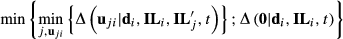
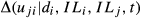
Our approach to decision‐making is to choose the sending location and inventory‐type quantities (if any) for the transshipment to minimize the expected costs incurred over any large horizon H under an assumption that no transshipments are made following the current decision. We fix horizon H to be any real number in excess of

{max}_{i} T_{i}

. If the current excess demand z _i at location i occurring at time t is met in whole or in part through a transshipment of u _jix ≤ IL _jx units of type x stock from j, 1 ≤ x ≤ X, then the costs to be incurred at both i and j over the time interval (t, t + H) may be computed. For sending location j, this total expected cost is given by the expression

\begin{matrix} R_{j i}^{f} + \sum_{x = 1}^{X} [R_{j i x}^{u} \cdot u_{j i x} + v_{j x} {I L_{j x} - u_{j i x}, t, t_{j} (t)}] \\ + v_{j} {t + t_{j} (t), t + H}, \end{matrix}

(14)

where the quantities v _jx{·,·,·} are computed as above and v _j{t + t _j(t), t + H} is the expected cost incurred at location j under no transshipments from the time of the first replenishment after t (at time t + t _j(t)) until the end of the horizon (at t + H). Please note that this latter quantity is independent of the decision made at the current epoch t. The expression in Equation 14 disaggregates the total expected cost incurred at location j over horizon H into the immediate cost of the transshipment (first two terms), the subsequent expected inventory cost until the first replenishment (third term) and the expected cost from the first replenishment to the end of the horizon (fourth term). Similarly, the total expected cost incurred over the horizon H at location i may be expressed as

\begin{matrix} \sum_{x = 1}^{X} [L_{i x} \cdot {(I L_{i x}^{+} - d_{i x} + u_{j i x})}^{-} + v_{i x} {{\tilde{I L}}_{i x} (u_{j i x}), t, t_{i} (t)}] \\ + v_{i} {t + t_{i} (t), t + H}, \end{matrix}

(15)

where

{\tilde{I L}}_{i x} (u_{j i x})

represents the inventory level of item x at location i after demand and transshipment. Under the lost sales model

{\tilde{I L}}_{i x} (u_{j i x}) = {(I L_{i x} + u_{j i x} - d_{i x})}^{+}

and the first term in Equation 15 is the one‐off cost associated with any residual unmet demand. However, under the backordered sales model, inventory levels are not restricted to be positive and

{\tilde{I L}}_{i x} (u_{j i x}) = I L_{i x} + u_{j i x} - d_{i x}

. The backorder costs for each item of unmet demand apply for the remaining time until the next replenishment and these are absorbed into the second term in Equation 15. Finally, for any location k ≠ i, j which is not a party to the transshipment, the total expected cost over the horizon H may be denoted V _k and written

V_{k} = \sum_{x = 1}^{X} v_{k x} {I L_{k x}, t, t_{k} (t)} + v_{k} {t + t_{k} (t), t + H} .

(16)

Hence, aggregating over locations using Equations (14)–(16), the total expected cost incurred across the entire network over horizon H may be expressed as

\begin{matrix} R_{j i}^{f} + \sum_{x = 1}^{X} [R_{j i x}^{u} \cdot u_{j i x} + L_{i x} \cdot {(I L_{i x}^{+} - d_{i x} + u_{j i x})}^{-} \\ + v_{i x} {{\tilde{I L}}_{i x} (u_{j i x}), t, t_{i} (t)} + v_{j x} {I L_{j x} - u_{j i x}, t, t_{j} (t)} \\ - v_{i x} {I L_{i x}, t, t_{i} (t)} - v_{j x} {I L_{j x}, t, t_{j} (t)}] + \sum_{k = 1}^{N} V_{k} . \end{matrix}

(17)

The total expected cost of making no transshipments either at t or throughout (t, t + H) is

\sum_{x = 1}^{X} [L_{i x} \cdot {(I L_{i x}^{+} - d_{i x})}^{-} + v_{i x} {{\tilde{I L}}_{i x} (0), t, t_{i} (t)} - v_{i x} {I L_{i x}, t, t_{i} (t)}] + \sum_{k = 1}^{N} V_{k} .

(18)

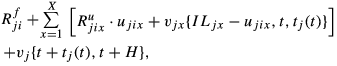
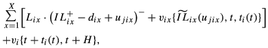
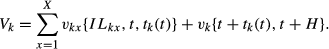
Our decision will be taken to secure the smallest possible value of the costs in Equations 17 or 18. To express this more succinctly, we develop the index

Δ (u_{j i} | d_{i}, {IL}_{i}, {IL}_{j}, t)

to reflect the benefit of making a transshipment of size u _ji ≡ {u _jix, 1 ≤ x ≤ X} at time t from j to i when a demand d _i results in a shortage at i and the inventory levels at i and j are IL _i and IL _j, respectively. We write

\begin{matrix} Δ (u_{j i} | d_{i}, {IL}_{i}, {IL}_{j}, t) = R_{j i}^{f} \\ + \sum_{x = 1}^{X} [R_{j i x}^{u} \cdot u_{j i x} + L_{i x} \cdot {(I L_{i x}^{+} - d_{i x} + u_{j i x})}^{-} \\ + v_{i x} {{\tilde{I L}}_{i x} (u_{j i x}), t, t_{i} (t)} + v_{j x} {I L_{j x} - u_{j i x}, t, t_{j} (t)} \\ - v_{i x} {I L_{i x}, t, t_{i} (t)} - v_{j x} {I L_{j x}, t, t_{j} (t)}] \end{matrix}

(19)

and

Δ (0 | d_{i}, {IL}_{i}, t) = \sum_{x = 1}^{X} [L_{i x} \cdot {(I L_{i x}^{+} - d_{i x})}^{-} + v_{i x} {{\tilde{I L}}_{i x} (0), t, t_{i} (t)} - v_{i x} {I L_{i x}, t, t_{i} (t)}]

(20)

for the no transshipment index. Our hybrid heuristic mandates a transshipment at t that achieves

min \{min_{j, u_{j i}} \{Δ (u_{j i} | d_{i}, {IL}_{i}, {IL}_{j}, t)\}; Δ (0 | d_{i}, {IL}_{i}, t)\},

(21)

where the choice of u _ji in the second minimization in Equation 21 is constrained by the stock levels at j and the requirement that stock levels at i should not go above S _ix(t + t _i(t)). Hence we require that

\begin{matrix} 0 \leq u_{j i x} \leq min \{I L_{j x}, S_{i x} (t + t_{i} (t)) - I L_{i x} + d_{i x}\}, \\ 1 \leq x \leq X, and 0 < u_{j i x} for some x . \end{matrix}

(22)

If the minimum in Equation 21 is achieved by

Δ (0 | d_{i}, {IL}_{i}, {IL}_{j}, t)

then no transshipment is made. Otherwise, the transshipment uses the pair

(j^{*}, u_{j i}^{*})

achieving the inner minimization.

The above approach is flexible and can accommodate a range of important model variants. We can, for example, easily extend the above to allow transshipments from more than a single location while in sections 4.2 and 4.4 we shall suppose that transshipments may be additionally constrained by the number or weight of items which may be included. Further, the possible “all or nothing” nature of demand mentioned in section 3 may be easily incorporated into the above by modifying costs in the analysis to reflect the fact that the demand d _i will not be lost in total following a shortage if and only if the triggered transshipment u _ji satisfies IL _ix + u _jix ≥ d _ix, 1 ≤ x ≤ X.

In practice, the above heuristic can be obtained with modest computational effort, especially so when X, the number of item types, is small. We recommend an online implementation of the minimization in Equation 21 which computes the key quantities

Δ (u_{j i} | d_{i}, {IL}_{i}, {IL}_{j}, t)

and

Δ (0 | d_{i}, {IL}_{i}, t)

as needed. In the event of a shortage at some location i, the relevant values of d _i, IL _i, and t are fixed and a search is prosecuted over locations j ≠ i and transshipment profiles u _ji. The building blocks for the computation of

Δ (u_{j i} | d_{i}, {IL}_{i}, {IL}_{j}, t)

are the availability of appropriate quantities of the form v _ix{IL _ix, t, t _i(t)} and v _jx{IL _jx, t, t _j(t)}. To obtain the complexity of computing these quantities, we write

{\hat{Λ}}_{i x} = {max}_{n} Λ_{i x} (t_{i}^{*} + n T_{i}, t_{i}^{*} + (n + 1) T_{i})

for the maximum mean x‐demand at location i during any review period, with

{\hat{M}}_{i x} = μ_{i x} \cdot {\hat{Λ}}_{i x} + 3 \sqrt{(μ_{i x}^{2} + σ_{i x}^{2}) \cdot {\hat{Λ}}_{i x}}

and

\hat{M} = {max}_{i, x} {\hat{M}}_{i x}

. The discussion of the computation of the quantities v _ix{IL _ix,t,t _i(t)} following Equation 10 yields the conclusion that their complexity is no worse than

O ({\hat{M}}^{2})

. Further, from Equation 19, we see that O(X) such quantities are needed to compute

Δ (u_{j i} | d_{i}, {IL}_{i}, {IL}_{j}, t)

for a single pair (j, u _ji). We now write

{\hat{S}}_{x} = {max}_{i, n} S_{i x} (t_{i}^{*} + n T_{i})

for the maximal replenishment level for items of type x at any location and time. It is straightforward that to compute all of the quantities in Equation 21 and to implement the minimization requires no more than

O (X {(N \hat{M} \prod_{x = 1}^{X} {\hat{S}}_{x})}^{2})

computations. In practice constraints on, for example, the size of vehicles available will mean that the number of feasible u _ji (where u _ji is feasible if u _jix x‐items, 1 ≤ x ≤ X, can be carried in a single transshipment from j to i) is much smaller than that calculation implies. Should F _ji be the number of distinct feasible transshipments u _ji from j to i and

\hat{F} = {max}_{j, i} F_{j i}

then no more than

O (X {(N \hat{M} \hat{F})}^{2})

computations would be needed to implement Equation 21.

Characterizations of the Hybrid Heuristic

In a setup as complex as considered here, it is perhaps unsurprising that simple characterizations of effective heuristics are challenging to develop. This subsection gives a brief account of some simple and intuitive features of the hybrid heuristic which are reasonably straightforward to establish.

Theorem 1 states that our hybrid rule is monotone in the sending location's stock levels. Hence, if the rule mandates a transshipment summarized by the pair

(j^{*}, u_{j^{*} i}^{*})

when the stock levels at j* are given by

{IL}_{j^{*}}

then under identical circumstances but where the stock levels at j* are uniformly above

{IL}_{j^{*}}

the rule continues to mandate a transshipment from j* with the stock transshipped uniformly no less that

u_{j^{*} i}^{*}

. The proof of Theorem 1 may be found in the paper's online Appendix. We use ⪯ to denote the componentwise weak ordering of two X‐vectors.

Theorem 1 The hybrid heuristic is monotone in the stock levels of the sending location

The index

Δ (u_{j i} | d_{i}, {IL}_{i}, {IL}_{j}, t)

is nonincreasing componentwise in IL _j for all fixed values of u _ji, d _i, IL _i and t.

If the minimization in Equation 21 is achieved by the pair

(j^{*}, u_{j^{*} i}^{*})

and if

{IL}_{j^{*}} ⪯ {IL}_{j^{*}}^{'}

, then

min \{min_{j, u_{j i}} \{Δ (u_{j i} | d_{i}, {IL}_{i}, {IL}_{j}^{'}, t)\}; Δ (0 | d_{i}, {IL}_{i}, t)\}

is achieved by some pair

(j^{*}, u_{j^{*} i}^{'})

where

u_{j^{*} i}^{*} ⪯ u_{j^{*} i}^{'}

It is possible to develop this result further as follows: Suppose now that we enhance the constraint set Equation 22 by adding a linear constraint of the form

\sum_{x = 1}^{X} w_{x} u_{j i x} \leq W_{j} .

(23)

For example, we could take w _x = 1 ∀x with W _j then the maximum number of items which can be carried in a single transshipment from j. Alternatively, w _x could be the weight of a single x‐item with W _j then the maximum total weight which can be carried in a single transshipment from j. Plainly part (a) of Theorem 1 continues to hold. However, we now have a weakened form of part (b) which states that if

I L_{j^{*} x}

increases from a point at which the heuristic mandates

(j^{*}, u_{j^{*} i}^{*})

then the supply location chosen will remain j* while the amount of item x supplied will not decrease.

It is also of interest to ask how decisions made by the hybrid heuristic change as the time to the next replenishment increases. The situation is complex but suppose we simplify matters by taking X = 1 and by supposing that all individual demands are for single items. Now consider how the transshipment decision made as a result of a shortage at i might change as the time to the next replenishment at location j increases from t _j(t) to t _j(t) + δ. The j‐term in an appropriate form of the expression in Equation 19 now changes from v _j{IL _j − u _ji,t,t _j(t)} − v _j{IL _j,t,t _j(t)} to v _j{IL _j − u _ji,t,t _j(t) + δ} − v _j{IL _j,t,t _j(t) + δ}. For small δ, this change in the value of the index

Δ (u_{j i} | d_{i}, I L_{i}, I L_{j}, t)

can be shown to be positive if and only if IL _j is less than some quantity ψ _j(t _j(t), u _ji) whose dependence on t _j(t) may be quite complex but which is increasing in u _ji. The interpretation of this is that location j becomes less attractive as a potential supplier as its replenishment recedes if its inventory is sufficiently small. In this case, the risk of future shortage costs at j exceeds the benefit of reduced holding costs. In general, increasing the review periods T _i, 1 ≤ i ≤ N, while keeping other aspects of the system unchanged, will put greater pressure on the availability of stock, which will in turn mean that effective approaches to making stock available when required will confer greater value. One simple observation is that, for constant demand rates, increasing the T _i, 1 ≤ i ≤ N, by multiplying them by a common factor while keeping other system features unchanged, is equivalent to leaving the T _i unchanged while increasing demand rates and holding cost rates by the same common factor. Either way, the results of the next subsection indicate that replenishment levels should be increased to reflect such changes. Increasing review periods while leaving all else about the system unchanged is somewhat akin to reducing replenishment levels to below economic optima.

On the Setting of Replenishment Levels

In the discussion above, replenishment levels are assumed given. In this subsection, we first give a brief account of the economically optimal setting of replenishment levels when locations operate independently and there is no pooling of inventory between them. The reason we begin a discussion of replenishment levels under a “no pooling” assumption is (a) because analytical progress is possible, and (b) to establish upper bounds on the search space for optimal replenishment levels for policies operating transshipments. Further, from our global assumption in section 3, we have a free choice of replenishment level at the start of each review period. From these considerations, we conclude that for the optimal setting of replenishment levels under no pooling it is sufficient to myopically consider how best to replenish a single location to minimize expected inventory costs incurred over a single review period. At the end of the subsection, we then describe how we deploy this analysis to establish an approach to the setting of replenishment levels in the context of the numerical study of our hybrid transshipment heuristic in section 5.

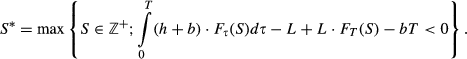
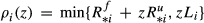
We can without loss of generality consider the optimal replenishment under no pooling of a single item x at a single location i and drop the identifier ix from the notation. In particular, we consider the choice of replenishment level S to minimize expected inventory costs v{S, 0, T}. We write S* for the optimal S‐value, satisfying

v {S^{*}, 0, T} = {min}_{S \in Z^{+}} {v {S, 0, T}}

. We use D _τ for the number of items demanded during [0, τ], F _τ for its distribution function, defined by F _τ(n) = P(D _τ < n),

n \in Z^{+}

, and

F_{τ}^{- 1}

for its inverse distribution function, namely

F_{τ}^{- 1} (β) = max {n; F_{τ} (n) < β}

, β ∈ [0, 1]. A proof of the following result may be found in the paper's online Appendix.

Proposition 1

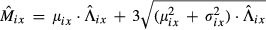
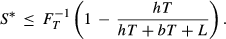
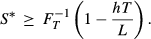
The optimal replenishment level S* in the absence of transshipments is given by

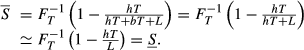
S^{*} = max \{S \in Z^{+}; \int_{0}^{T} (h + b) \cdot F_{τ} (S) d τ - L + L \cdot F_{T} (S) - b T < 0\} .

(24)

S* is bounded above as follows:

S^{*} \leq F_{T}^{- 1} (1 - \frac{h T}{h T + b T + L}) .

(25)

If L > hT > 0 then S* is bounded below as follows:

S^{*} \geq F_{T}^{- 1} (1 - \frac{h T}{L}) .

(26)

We shall refer to the upper and lower bounds on S* given in the above result as S and S , respectively. We readily conclude that for cases of the lost sales model for which hT≪L, S will be reasonably tight since then we have

\begin{matrix} \bar{S} & = F_{T}^{- 1} (1 - \frac{h T}{h T + b T + L}) = F_{T}^{- 1} (1 - \frac{h T}{h T + L}) \\ ≃ F_{T}^{- 1} (1 - \frac{h T}{L}) = \underset{̲}{S} . \end{matrix}

(27)

We now develop approximations to the upper bound S based on the normal distribution.

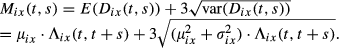
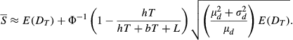
We can use the central limit theorem to develop a normal approximation to the distribution of the total demand D _T under the condition that the expectation E(D _T) is moderately large. Recall that we use μ _d and

σ_{d}^{2}

, respectively, for the mean and variance of the number of units demanded by a single individual. It then follows that E(D _T) = μ _dΛ(0, T) and

V a r (D_{T}) = (μ_{d}^{2} + σ_{d}^{2}) Λ (0, T) = (\frac{μ_{d}^{2} + σ_{d}^{2}}{μ_{d}}) E (D_{T})

and we conclude from Equation 25 that S is well approximated by

\bar{S} \approx E (D_{T}) + Φ^{- 1} (1 - \frac{h T}{h T + b T + L}) \sqrt{(\frac{μ_{d}^{2} + σ_{d}^{2}}{μ_{d}}) E (D_{T})} .

(28)

We now restore the item/location identifier ix. Features which will be present in the numerical examples in section 5 are a repeating demand pattern on a weekly cycle for all items at all locations and a review period equal to an integer number of weeks. These assumptions simplify things considerably. Replenishment levels S _ix, 1 ≤ i ≤ N, 1 ≤ x ≤ X, now need to be tailored to individual locations i and item types x but not to the times at which the replenishments are made. From the above analysis, a natural approach to the determination of replenishment levels would be to conduct an appropriate search using the above upper bounds for no pooling as a starting point. We would certainly expect that optimal replenishment levels under inventory pooling via transshipments to be somewhat lower than for no transshipments. Our numerical studies confirm this. Further, it is not unreasonable to assume common characteristics for inventory costs and for the nature of individual demands across locations. We can then suppose that replenishment levels take the form

S_{i x} = E (D_{i x T}) + α_{x} \sqrt{E (D_{i x T})}, 1 \leq i \leq N, 1 \leq x \leq X

(29)

and conduct a search over common α _x, 1 ≤ x ≤ X, to achieve costs which are close to minimizing.

The above discussion notwithstanding, our envisaged application domain frequently features city center locations where rents are high and space is limited. Hence it may not be possible to replenish at the levels suggested by the analysis of the cost model, as above. In light of this, it will be important to consider the impact of our heuristic transshipment policies when replenishment levels are set lower than cost optimal. In section 5, we shall consider the performance of our hybrid heuristic for both cases when replenishment levels are set in a cost minimizing fashion and when rather lower levels are assumed because of space constraints.

A Lower Bound on Achievable Costs When All Locations Replenish simultaneously

The intractability of our decision problem means that it is only possible to compare the cost performance of our heuristic directly with optimal in small problems. For certain cases, we are able to further strengthen our analyses by developing lower bounds on the expected cost rate achievable under any policy. Such is the complexity of our setup that we can only achieve simple and effective bounds for cases in which (i) all locations are replenished simultaneously, (ii) all locations share a common holding cost rate for each item type, namely h _x, 1 ≤ x ≤ X, and (iii) a constraint of the form in Equation 23 delimits transshipments from each location. To illustrate the approach simply, we shall take X = 1 and drop the item identifier x in what follows. We shall also focus on the lost sales model. Extensions to X > 1 and/or to backorder costs are straightforward.

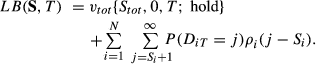
We shall obtain a lower bound LB(S, T) on the costs achievable under any policy in a single review period of length T and with replenishment levels given by the N‐vector S. We obtain LB(S, T) by developing lower bounds on the two elements of inventory costs, namely holding and shortage costs. To obtain a lower bound on holding costs, we imagine the network operating as a single location with aggregate replenishment level

S_{tot} = \sum_{i = 1}^{N} S_{i}

and aggregate demand rate

λ_{tot} (t) = \sum_{i = 1}^{N} λ_{i} (t)

. This method of accounting for stock gives a lower bound on the actual stock present and the corresponding holding costs at all time points as it defers lost sales to the last moment. Using the quantities S _tot and λ _tot(t) in Equation 9, we obtain a lower bound on holding costs

v_{t o t} {S_{t o t}, 0, T; hold} = \sum_{j = 1}^{S_{t o t}} \sum_{n = 1}^{j} h \cdot (A_{t o t} (n, 0, T) + T \cdot B_{t o t} (n, 0, T)) \cdot P_{j}^{n} .

(30)

To obtain a lower bound on shortage costs, we first use

R_{* i}^{f}

and

R_{* i}^{u}

as, respectively, the smallest fixed and unit costs associated with transshipments to location i. Further, using Equation 23 with X = 1, we have an inequality wu _ji ≤ W _j delimiting the size of transshipments from j to i and we write

W = max_{j} \frac{W_{j}}{w}

for the maximum quantity which can be handled by a single transshipment. Condition now on the event that location i faces an aggregate shortage z over a single review period. This shortage will incur costs which are a combination of those due to transshipments and lost sales. It can be seen that when W < ∞, a lower bound on shortage costs at location i is given by the quantity

ρ_{i} (z) = min_{0 \leq u \leq z} \{⌈\frac{u}{W}⌉ R_{* i}^{f} + u R_{* i}^{u} + (z - u) L_{i}\} .

(31)

When W = ∞, the appropriate expression is

ρ_{i} (z) = min {R_{* i}^{f} + z R_{* i}^{u}, z L_{i}}

. Combining the above elements yields Proposition 2 in which D _iT is the total demand at i in a single review period.

Proposition 2

A lower bound on the network costs incurred over a review period of length T and with replenishment levels S is given by

\begin{matrix} L B (S, T) & = v_{t o t} {S_{t o t}, 0, T; hold} \\ + \sum_{i = 1}^{N} \sum_{j = S_{i} + 1}^{\infty} P (D_{i T} = j) ρ_{i} (j - S_{i}) . \end{matrix}

(32)

Experimentation

To test the performance of the new hybrid policy an extensive simulation study has been carried out. We first explore how different heuristic approaches perform compared to optimal for small problems. Given the complexity of the decision problem, this analysis is restricted to a single item in a network with three locations. Alongside the new hybrid policy (H), we test the performance of no pooling (NP) in which no transshipments occur and complete pooling (CP) in which transshipments to meet shortages are designed on a minimum immediate cost basis. We also study a standard reactive policy (R) which was adapted from Archibald et al. (2010). All policies were applied under the same conditions using common random numbers. For the optimal policy, the cost rate was determined via dynamic programming. Table 2 summarizes the optimality gaps obtained for the above policies and highlights how policy H closes the gap to optimal considerably.

In addition to the evaluation of the hybrid policy H via comparisons to optimal we use Monte Carlo simulation to study its performance in larger networks with 10 and 50 locations and two distinct item types. In Tables 3–7, the cost rate performances of the policies mentioned above are compared in these larger networks along with that of an artificial policy (Hpar) which runs the decision rule H for each item type separately before aggregating costs. Comparing H to Hpar shows the improvement achieved by modeling item types together and allowing coordinated proactive transshipments of multiple item types at each decision epoch. In Table 8, the cost rates incurred by NP, CP, R, and H are compared with the lower bound established in section 4.4 for problems with 10 locations which are replenished simultaneously. Subsequent studies aim to assess the benefits offered by our demand modeling generality (Table 9) and to characterize competing transshipment heuristics in terms of the size, frequency, and timing of transshipments (Figure 1).

Figure 1

Timing and Size of Transshipments for Different Policies

In all of the numerical studies reported in this section, we shall take the unit of time to be one day and shall assume that stock is replenished on a weekly basis (T _i = 7,∀i). Successive replenishments at location i occur at

r_{i} + 7 m, m \in N

, for some offset r _i ∈ [0, 7), 1 ≤ i ≤ N. We also assume a weekly demand pattern. We write λ _i for the mean number of customer arrivals at i per week and φ _ik for the long run proportion of customers who arrive during day k ∈ {1,…,7} of the week. Hence the customer arrival rate at i during k is λ _i φ _ik. These choices are informed by the motivating application concerning the sale of car parts. Note that the parameters λ _i and φ _ik are chosen constant here, but our approach accommodates varying these for successive replenishment cycles to model any trend in demand. In what follows we shall use D‐Pat as an abbreviation for the pattern of weekly demands λ in the network and P‐Pat for the associated phase patterns φ.

In our numerical studies, we assign each location to one of three similarly sized groups. Locations within group g have a common customer arrival rate

λ_{\bar{g}}

and we assume a common phase pattern φ _k, 1 ≤ k ≤ 7, across all locations. Table 1 contains details of the D‐Pat and P‐Pat applied. We further take f _ixd = 0.8(1 − 0.8)^d−1, d ≥ 1, as our model for type‐x demand per customer at i, with an associated mean of 1.25. With the exception of the simultaneous replenishment setting of Table 8, the offsets r _i determining the times of location replenishments are drawn independently and uniformly from the interval [0, 7). Transshipment costs are characterized by the triple (R ^fix, R ^dist, R ^u). The fixed element of the cost of a transshipment from j to i is given by

R_{j i}^{f} = R^{fix} + ξ_{j i} R^{dist}

, while the per unit cost is

R_{j i x}^{u} = R^{u}

for all choices of j,i and x. The factor ξ _ji is the normalized distance between locations j and i. Since throughout our experimentation, we found that the lost sales and backordered sales models produced comparable results, we include results only for the former.

Table 1

Overview of Demand and Phase Patterns Used

Weekly demand	Values	Phase pattern	Values
D‐Pat 1	$λ_{\bar{1}} = 20$ , $λ_{\bar{2}} = 20$ , $λ_{\bar{3}} = 20$	P‐Pat 0	$φ_{k} = \frac{1}{7} \forall k$ (Constant/Stationary)
D‐Pat 2	$λ_{\bar{1}} = 25$ , $λ_{\bar{2}} = 20$ , $λ_{\bar{3}} = 15$	P‐Pat 1	φ = (0.100,0.250,0.250,0.100,0.100,0.100,0.100)
D‐Pat 3	$λ_{\bar{1}} = 30$ , $λ_{\bar{2}} = 20$ , $λ_{\bar{3}} = 10$	P‐Pat 2	φ = (0.050,0.375,0.375,0.050,0.050,0.050,0.050)
		P‐Pat 3	φ = (0.150,0.350,0.200,0.075,0.075,0.075,0.075)

In all experiments reported in this section, excepting only those in Table 5, we assume that holding and lost sales cost rates do not vary with location and item type. When this is the case, we also take the holding cost rate to be the unit in which all costs are measured. Hence, we have h _ix = 1 and L _ix = L for all choices of i,x. For these cases, we assume from the discussion in section 4.3 leading to (29) that replenishment levels take the form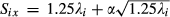

S_{i x} = 1.25 λ_{i} + α \sqrt{1.25 λ_{i}}

, where the parameter α is either optimized in the manner described in section 4.3 or is set equal to 1 or 1.5. To demonstrate that our results are not dependent on assumptions of homogeneity of inventory and transshipment costs across item types, we include in Table 5 a set of results where this is not the case. For all of the values reported in Tables 3–9 and Figure 1, 50 simulation repetitions were performed with each running for 200 replenishment periods (weeks).

Table 2 summarizes results obtained for different heuristic policies expressed as the deviation (percentage excess) from the optimal cost rate. These are all three location problems with replenishment levels set by taking α = 1 in a suitable form of Equation 29. Experiments were carried out for all combinations of the demand and phase patterns in Table 1 and three levels of both lost sales penalties and transshipment costs. This yields 108 problem configurations in all. We present average figures for the results obtained for different cost levels as well as the worst case. Please note that the hybrid heuristic H closes the greater part of the suboptimality gap left by other heuristics.

Table 2

Suboptimality Gap Results for a Three Location Network Using α = 1

Parameter		Suboptimality gap for policy (%)
Parameter		NP	CP	R	H
L	20	10.09	4.98	4.40	0.14
	60	76.72	15.00	13.47	0.54
	100	133.63	12.43	12.18	0.79
(R ^fix,R ^dist,R ^u)	(10, 40, 0)	64.28	12.46	11.52	0.51
	(10, 40, 1)	60.13	11.21	10.16	0.41
	(5, 20, 1)	96.04	8.75	8.36	0.55
Worst case		126.80	15.84	15.48	1.14

The 10 location experiments whose results are given in Tables 3 and 4 were conducted on 10 randomly generated maps. The experiments were as described above and the relevant model parameters are given in the tables. We include results for just one phase/demand pattern since we found that varying P‐Pat and D‐Pat had little impact on the relative performance of the heuristic policies. The tables give values of the cost per week incurred under different policies and for a variety of problem contexts also record the percentage cost reduction achieved by H in comparison to other policies. Table 3 considers contexts in which limited storage space dictates low replenishment levels (α set to 1 in a suitable form of Equation 29) while in Table 4, the value of α has been chosen to achieve a minimum cost rate for each policy. This optimal value lies in the range [1.3,1.6] for CP, [1.2,1.6] for R and [0.9,1.1] for H, with larger optimizing α obtained when lost sales penalties and/or transshipments costs are high. For policy NP, optimal values of α were obtained from Equation 24. We can infer that the new hybrid policy allows for considerably lower levels of safety stock compared to other policies, thus keeping holding costs low. This is especially important for inventory systems where holding costs constitute a major part of the operating costs.

Table 3

Lost Sales Results for 10 Locations Using α = 1 (D‐Pat 3, P‐Pat 2)

Parameter		Cost per period using policy					Improvement of H over (%)
(R ^fix,R ^dist,R ^u)	L	NP	CP	R	Hpar	H	NP	CP	R	Hpar
(10, 40, 0)	20	543.27	482.82	465.12	405.08	389.44	39.50	23.98	19.43	4.01
	60	975.55	496.37	485.33	415.63	397.97	145.13	24.72	21.95	4.44
	100	1407.83	496.37	492.86	419.73	401.01	251.08	23.78	22.91	4.67
(10, 40, 1)	20	543.27	492.38	474.25	422.86	409.69	32.60	20.18	15.76	3.21
	60	975.55	511.53	496.73	434.56	419.96	132.30	21.80	18.28	3.48
	100	1407.83	511.53	504.11	439.18	423.72	232.25	20.72	18.97	3.65
(5, 20, 1)	20	543.27	422.81	412.67	384.83	378.69	43.46	11.65	8.97	1.62
	60	975.55	422.81	420.41	391.05	384.45	153.75	9.98	9.35	1.72
	100	1407.83	422.81	424.68	393.09	386.30	264.44	9.45	9.94	1.76

We also observe that the relative performance of the hybrid policy is particularly strong for higher shortage costs which is also very important for industries where high penalties apply for unmet customer demand. For high levels of shortage costs, it is notable that for non‐simultaneous replenishments, as is the case here, the myopic policy CP in some cases outperforms policy R. This is due to the fact that the purely reactive quasi‐myopic approach overestimates future shortage costs at locations where the remaining time until the next replenishment is long and thus produces inferior decisions. This deficiency is completely removed by the hybrid approach.

Table 4

Lost Sales Results for 10 Locations Using Respective Optimal Values of α (D‐Pat 3, P‐Pat 2)

Parameter		Cost per period using policy					Improvement of H over (%)
(R ^fix,R ^dist,R ^u)	L	NP	CP	R	Hpar	H	NP	CP	R	Hpar
(10, 40, 0)	20	465.90	440.98	437.62	400.84	389.28	19.68	13.28	12.42	2.97
	60	529.36	443.72	443.43	409.43	395.90	33.71	12.08	12.01	3.42
	100	561.26	443.72	445.40	411.98	398.32	40.91	11.40	11.82	3.43
(10, 40, 1)	20	465.90	444.10	441.62	414.14	405.39	14.93	9.55	8.94	2.16
	60	529.36	447.79	447.57	420.75	413.38	28.06	8.33	8.27	1.78
	100	561.26	447.79	449.05	423.71	416.51	34.76	7.51	7.81	1.73
(5, 20, 1)	20	465.90	412.11	408.05	384.83	377.72	23.35	9.11	8.03	1.88
	60	529.36	412.11	413.25	391.05	383.97	37.87	7.33	7.63	1.85
	100	561.26	412.11	415.50	393.09	385.83	45.47	6.81	7.69	1.88

Table 5 shows results from a set of experiments in which we have introduced item cost heterogeneity and set h _i1 = 0.5, h _i2 = 1.5, L _i1 = L, L _i2 = 2L,

R_{j i 1}^{u} = R^{u}

R_{j i 2}^{u} = 3 R^{u}

. Other aspects of the studies are unchanged from those reported in Tables 3 and 4. The reader will note that the introduction of item cost heterogeneity has not materially affected the nature of the results.

Table 5

Lost Sales Results for 10 Locations With Heterogeneous Item Types Using α = 1 (D‐Pat 3, P‐Pat 2)

Parameter		Cost per period using policy					Improvement of H over (%)
(R ^fix,R ^dist,R ^u)	L	NP	CP	R	Hpar	H	NP	CP	R	Hpar
(10, 40, 0)	20	640.54	483.70	466.90	403.54	387.54	65.28	24.81	20.48	4.13
	60	1277.52	491.56	485.47	413.39	395.25	223.22	24.37	22.83	4.59
	100	1914.50	491.56	493.35	416.79	397.76	381.32	23.58	24.03	4.79
(10, 40, 1)	20	640.54	509.91	488.02	437.60	425.74	50.45	19.77	14.63	2.78
	60	1277.52	520.87	507.38	450.20	437.67	191.89	19.01	15.93	2.86
	100	1914.50	520.87	515.07	454.70	441.78	333.36	17.90	16.59	2.92
(5, 20, 1)	20	640.54	432.16	420.64	397.99	393.36	62.84	9.86	6.94	1.18
	60	1277.52	432.16	428.79	405.12	400.99	218.59	7.77	6.93	1.03
	100	1914.50	432.16	432.74	407.41	403.41	374.58	7.13	7.27	0.99

To evaluate how the benefits of the hybrid policy scale with the size of the network, experiments were conducted using a network with 50 locations. Here, geographical data on 50 branches of a car parts dealer were used. Tables 6 and 7 report a set of results equivalent to those for 10 locations in Tables 3 and 4. In the determination of replenishment levels, the parameter α was both set to be 1 (Table 6) and optimized (Table 7). The larger number of locations means that the chance of a suitable sending location when a shortage occurs is enhanced. Hence, it is true for all transshipment policies that safety stock levels, as reflected by the optimal α values computed for Table 7 were significantly reduced compared to those for the 10 location problems of Table 4. Optimal α are now in the range [1.0,1.3] for CP, [0.9,1.3] for R and [0.6,1.0] for H. We can see that with regard to choosing α optimally the benefit of H observed earlier is increased. The importance of transshipments per se is seen in the dominance of all transshipment policies over NP.

Table 6

Lost Sales results for a 50 Location Network Using α = 1 (D‐Pat 3, P‐Pat 2)

Parameter		Cost per period using policy					Improvement of H over (%)
(R ^fix,R ^dist,R ^u)	L	NP	CP	R	Hpar	H	NP	CP	R	Hpar
(10, 40, 0)	20	2758.67	2205.63	2148.63	1914.70	1867.21	47.74	18.12	15.07	2.54
	60	4914.75	2205.92	2160.05	1940.75	1891.54	159.83	16.62	14.20	2.60
	100	7070.83	2205.92	2168.15	1954.36	1902.60	271.64	15.94	13.96	2.72
(10, 40, 1)	20	2758.67	2270.44	2203.62	2007.06	1971.19	39.95	15.18	11.79	1.82
	60	4914.75	2270.84	2214.50	2040.50	2007.00	144.88	13.15	10.34	1.67
	100	7070.83	2270.84	2222.43	2057.92	2023.44	249.45	12.23	9.83	1.70
(5, 20, 1)	20	2758.67	2000.74	1966.62	1891.57	1878.34	46.87	6.52	4.70	0.70
	60	4914.75	2000.74	1975.49	1917.52	1906.90	157.73	4.92	3.60	0.56
	100	7070.83	2000.74	1980.79	1928.37	1918.16	268.63	4.31	3.26	0.53

It is clear from the results obtained in Tables 2–7 that the hybrid policy improves significantly upon the competing heuristics. For networks larger than three locations, the full potential of applying the hybrid approach remains unknown as an optimal solution cannot be determined for use as a comparator. Section 4.4 introduced a lower bound for the cost per period achievable under any policy. For this setup, an assumption of simultaneous replenishment of all locations is required. The results presented in Table 8 use the same underlying parameters as before with the exception that the offset r _i of the weekly repeating replenishment pattern is set to zero for all i. To allow a common lower bound for all policies a fixed value of α is used. This was set at level α = 1.5 to achieve a reasonably strongly performing set of replenishment levels for all the policies. The evidence of Table 8 is that the hybrid policy is close to optimal for the cases considered. The deviation from the lower bound ranges from roughly 1.5% to 3.5% for the hybrid policy. As was the case in Table 2, Table 8 again makes clear that the hybrid heuristic H closes the major part of the suboptimality gap left by the competing heuristics in these larger problems. Further, upon close inspection, the reader should observe that the lower bound developed in section 4.4 applies to all approaches to stock rebalancing between (simultaneous) replenishments, not simply those triggered by shortages of the kind considered here. Hence, for the problems in Table 8, heuristic H is competitive with a wide range of possible approaches including those which take a different approach to proactive transshipment and/or which allow simultaneous transshipments from more than a single location.

Table 7

Lost Sales Results for a 50 Location Network Using Respective Optimal Values of α (D‐Pat 3, P‐Pat 2)

Parameter		Cost per period using policy					Improvement of H over (%)
(R ^fix,R ^dist,R ^u)	L	NP	CP	R	Hpar	H	NP	CP	R	Hpar
(10, 40, 0)	20	2374.59	2144.02	2121.86	1903.20	1838.37	29.17	16.63	15.42	3.53
	60	2688.90	2144.07	2129.20	1932.36	1872.02	43.64	14.53	13.74	3.22
	100	2842.91	2144.07	2134.19	1947.72	1887.01	50.66	13.62	13.10	3.22
(10, 40, 1)	20	2374.59	2178.19	2164.37	2007.06	1966.21	20.77	10.78	10.08	2.08
	60	2688.90	2178.27	2159.85	2040.50	2005.06	34.11	8.64	7.72	1.77
	100	2842.91	2178.27	2162.88	2057.92	2023.44	40.50	7.65	6.89	1.70
(5, 20, 1)	20	2374.59	2000.74	1963.43	1864.19	1838.16	29.18	8.85	6.82	1.42
	60	2688.90	2000.74	1974.48	1896.01	1875.46	43.37	6.68	5.28	1.10
	100	2842.91	2000.74	1981.03	1908.50	1888.22	50.56	5.96	4.92	1.07

To assess the contribution made to the results by our incorporation of non‐homogeneous demand, we designed a hybrid heuristic (Ave) on the basis of a false assumption of homogeneous demand at a suitable weekly rate when in fact phase patterns 1–3 apply. In Table 9, find cost rates which compare H with Ave over a set of cases similar to those used in Tables 3 and 4, but for a single‐item model and with replenishment levels set by taking α = 1 and α = 1.5. From our entire set of results, we note that a cost rate benefit of up to 3% can be achieved by correctly incorporating demand seasonality in the model. In an unreported study available from the authors, they demonstrate the superiority of H over competing heuristics even in the case of pure Poisson demand which has been a standard assumption in the literature hitherto.

Table 8

Performance Analysis for 10 Locations Using the Derived Lower Bound and α = 1.5 (D‐Pat 3, P‐Pat2)

Parameter		Deviation from lower bound (%)
(R ^fix,R ^dist,R ^u)	L	NP	CP	R	H
(10, 40, 0)	20	19.06	12.36	11.84	1.47
	60	68.48	13.84	13.20	1.91
	100	117.90	13.84	13.31	2.16
(10, 40, 1)	20	17.72	12.01	11.50	2.52
	60	66.56	13.85	13.15	3.17
	100	115.42	13.85	13.25	3.54
(5, 20, 1)	20	21.24	7.19	6.77	1.94
	60	71.58	7.19	6.87	2.49
	100	121.91	7.19	6.95	2.76

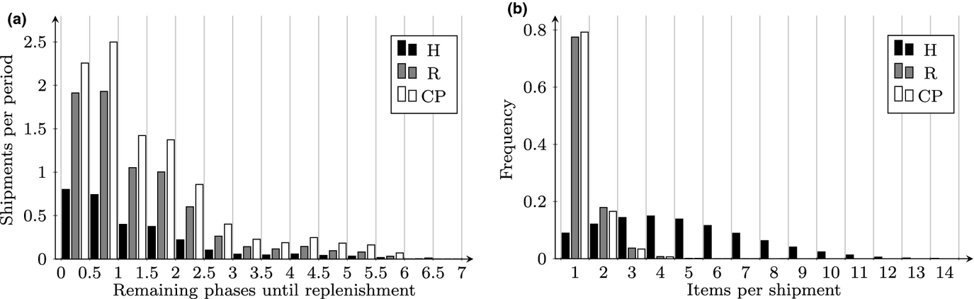
We finally analyze the nature of the policies for the set of experiments reported in Table 3. The left hand plot of Figure 1 shows how often transshipments were made under the policies CP, R, and H and the phases remaining until the next replenishment at the receiving location. We can see that under the hybrid policy, transshipments are much less frequent than for policies CP and R. Particularly striking is the extent to which H mitigates the spike in the frequency of transshipments which occurs for CP and R at the end of a review period. This is reflected in our cost‐benefit analyses as fixed costs for transshipments increase. We can also see that CP has an increased transshipment frequency compared to R due to its myopic nature. The right hand plot of Figure 1 reports the size of transshipments made under each policy. While in the majority of cases CP and R ship only one item to meet a shortage, policy H makes significantly larger transshipments. This not only prevents future transshipments due to the reduced chance of stockouts, it also makes efficient use of the capacity of vehicles and exploits the dominance of fixed over variable costs.

Table 9

Non‐homogeneous Benefit Analysis for 10 Locations in a Single Item Network (D‐Pat 3, P‐Pat 3)

		α = 1			α = 1.5
Parameter		Cost		Gain	Cost		Gain
(R ^fix,R ^dist,R ^u)	L	Ave	H	(%)	Ave	H	(%)
(10, 40, 0)	20	177.7	173.0	2.66	165.6	162.7	1.75
	60	188.0	182.5	2.88	168.9	165.2	2.16
	100	193.7	188.7	2.57	170.1	166.6	2.06
(10, 40, 1)	20	190.2	185.1	2.69	173.4	170.0	1.96
	60	201.6	195.6	3.01	177.5	173.2	2.41
	100	207.6	202.1	2.65	179.0	174.9	2.27
(5, 20, 1)	20	162.2	158.7	2.14	159.1	156.5	1.59
	60	169.0	166.0	1.77	161.1	158.8	1.45
	100	173.7	171.1	1.48	161.9	159.9	1.28

Conclusion

The hybrid policy improves significantly upon a reactive policy and other heuristics when a substantial part of the transshipment cost is fixed. This is particularly relevant for networks which are spread over a wide geographic area where the cost of transshipping will be predominantly determined by distance and time travelled rather than the amount transported. The main improvement lies in the fact that fewer transshipments of larger size are made thus making efficient use of the resources involved. Not only will reducing the frequency of transshipments reduce costs, it also reflects a more strategic approach to stock rebalancing and will reduce the extent to which stock is shuffled repeatedly between locations. It has also emerged that deployment of the hybrid policy permits major savings in inventory costs through reductions in the levels of safety stock required. We have provided evidence that our hybrid heuristic not only improves upon previous proposals but also comes close to optimal. In particular, we have provided evidence that this policy achieves most of the benefits available from the pooling of inventory without the need to consider rebalancing across all locations simultaneously, with all of the organisational difficulties that entails.

In addition to considerable cost savings, our approach also enables a much greener business operation as the capacity of transport vehicles is used more efficiently with fewer journeys. Allowing compound non‐homogeneous demand provides further performance gains and greater precision in the policy's application. Our approach enables a very general setting allowing multiple item types where demand is drawn from a general multivariate distribution. Further, a more flexible modeling of shortage costs is offered. This increased generality allows the hybrid policy to exploit the benefits offered by economies of scale in a wide range of practical settings.

References

Agrawal

Chao

Seshadri

. 2004. Dynamic balancing of inventory in supply chains. Eur. J. Oper. Res. 159(2): 296–317.

Archibald

T. W.

2007. Modelling Replenishment and Transshipment Decisions in Periodic Review Multilocation Inventory Systems. J. Oper. Res. Soc. 58(7): 948–956.

Archibald

T. W.

Sassen

S. A. E.

Thomas

L. C.

. 1997. An Optimal Policy for a Two Depot Inventory Problem with Stock Transfer. Manage. Sci. 43(2): 173–183.

Archibald

T. W.

Black

D. P.

Glazebrook

K. D.

. 2010. The use of simple calibrations of individual locations in making transshipment decisions in a multi‐location inventory network. J. Oper. Res. Soc. 61(2): 294–305.

Axsäter

2003. A New Decision Rule for Lateral Transshipments in Inventory Systems. Manage. Sci. 49(9): 1168–1179.

Çömez

Stecke

K. E.

Çakanyıldırım

. 2012. Multiple in‐cycle transshipments with positive delivery times. Prod. Oper. Manag. 21(2): 378–395.

Gerchak

and Henig

. 1986 An inventory model with component commonality. Oper. Res. Lett. 5(3): 157–160.

Gross

. 1963. Centralized inventory control in multilocation supply systems. Scarf

Gilford

Shelly

(, eds.) Multistage Inventory Models and Techniques. Stanford University Press, Stanford, CA, 47–84.

Herer

Y. T.

Tzur

. 2001 The dynamic transshipment problem. Nav. Res. Log. 48(5): 386–408.

10.

Herer

Y. T.

Tzur

. 2003. Optimal and heuristic algorithms for the multi‐location dynamic transshipment problem with fixed transshipment costs. IIE Trans. 35(5): 419–432.

11.

Kranenburg

A. A.

van Houtum

G. J.

2009 A new partial pooling structure for spare parts networks. Eur. J. Oper. Res. 199(3): 908–921.

12.

Krishnan

K. S.

Rao

V. R.

. 1965. Inventory control in N warehouses. J. Ind. Eng. 16(3): 212‐215.

13.

Lee

Y. H.

Jung

J. W.

Jeon

Y. S.

. 2007 An effective lateral transshipment policy to improve service level in the supply chain. Int. J. Prod. Econ. 106(1): 115–126.

14.

Lien

R. W.

Iravani

S. M. R.

Smilowitz

, and Tzur

. 2011. An Efficient and Robust Design for Transshipment Networks. Prod. Oper. Manag. 20(5): 699–713.

15.

Paterson

Kiesmüller

Teunter

Glazebrook

. 2010. Inventory models with lateral transshipments: A review. Eur. J. Oper. Res. 210(2): 125–136.

16.

Paterson

Teunter

Glazebrook

. 2012. Enhanced lateral transshipments in a multi‐location inventory system. Eur. J. Oper. Res. 221(2): 317–327.

17.

Rao

U. S.

Swaminathan

J. M.

Zhang

. 2004. Multi‐product inventory planning with downward substitution, stochastic demand and setup costs. IIE Trans. 36(1): 59–71.

18.

Robinson

L. W.

1990. Optimal and approximate policies in multiperiod, multilocation inventory models with transshipments. Oper. Res. 38(2): 278–295.

19.

Swaminathan

J. M.

Tayur

S. R.

. 1998. Managing broader product lines through delayed differentiation using vanilla boxes. Manage. Sci. 44 (12): S161–S172.

20.

Wong

van Houtum

G. J.

Cattrysse

van Oudheusden

. 2005. Simple, efficient heuristics for multi‐item multi‐location spare parts systems with lateral transshipments and waiting time constraints. J. Oper. Res. Soc. 56(12): 1419–1430.

21.

Yao

D. D.

Zheng

. 2011. Optimal control of replenishment and substitution in an inventory system with nonstationary batch demand. Prod. Oper. Manag. 20(5): 727–736.

22.

Zhao

Ryan

J. K.

Deshpande

. 2008. Optimal Dynamic Production and Inventory Transshipment Policies for a Two‐Location Make‐to‐Stock System. Oper. Res. 56(2): 400–410.