Promotion Planning and Supply Chain Contracting in a High–Low Pricing Environment

Introduction

Empirical literature finds that only 18% of promotion campaigns are profitable (Srinivasan et al. 2004). In an efficient consumer response (ECR) study among Australasian members of the fast‐moving consumer goods (FMCG) industry, it is reported that out‐of‐stock rates more than double during promotions (ECR Australia 2010). Given the number of the unprofitable and thus potentially inefficient promotions, firms in this industry expect substantial welfare improvement from efficient promotions (Hua 2011). Price promotions are critical in the management of fast‐moving consumer goods. For example, 75%–85% of the total sales volume of diapers occur during price promotions (Huchzermeier et al. 2002).

In discussions about efficient promotions, a senior executive of Germany's largest retailer brought the following challenge to our attention. A retailer who plans a price promotion faces a fundamental issue: She cannot perfectly predict the extent to which demand will respond to the reduced prices. Retailers thus establish inventory levels based on a historic forecast of demand that is noisy. A retailer who overestimates demand is left with excess inventory or end‐of‐period coverage (EPC), which is wasteful. In our context, reducing excess inventory is a key objective of retailers, as it inhibits the introduction of new products (e.g., the launch of a detergent with a different scent). If the retailer underestimates demand, however, then consumers may face empty shelves and possibly buy elsewhere (e.g., at discounters), hence the retailer faces lost sales (Arminger 2008, Hopp 2008). If the planned inventory happens to achieve the profit‐maximizing supply quantity, with inventory clearing at the end of the promotion period, then the promotion campaign is deemed “truly efficient,” because it results in zero lost sales and zero end‐of‐period coverage. The latter is a key objective of retailers who seek to ensure the success of promotional activity (ECR Australia 2010).

Modeling price promotions of FMCG requires some background on pricing and negotiation processes in this industry. Based on anecdotal evidence from discussions with senior executives from leading branded goods companies in Germany, retailers and manufacturers negotiate wholesale prices and other terms, such as service levels for emergency orders, once a year. The wholesale price usually cannot be altered during the year. In addition, retailers develop a year‐long promotion plan containing information on the timing of promotions but not on promotion (retail) prices. Thus, the decision to promote does not depend on the level of inventory held by the retailer. By law, the advance fixing of promotion prices is prohibited because it infringes on the right of retailers to determine their own prices (Mundt 2010). Wholesale prices and promotion timing are thus common knowledge, whereas retail prices are not determined in advance.

In their pricing strategy, retailers offer both deep and shallow discounts to attract price‐sensitive customers and to compete for market share (Bell et al. 2002, Wiehenbrauk 2010). Promotion prices are selected randomly before a promotion starts. Several models (Bell et al. 2002, Lal et al. 1996, Varian 1980, Wiehenbrauk 2010) show that random promotion pricing is optimal from a competitive point of view. Predictable pricing policies can be underbid and thus are dominated by random mixed strategies. For instance, Real—a major German retail chain—employs a tool developed by Comosoft to adjust retail prices until five minutes before printing promotional leaflets (Rück 2010). Without knowledge of even a planned retail price, it is impossible to predict demand perfectly. Thus, forecast errors are practically guaranteed by the retailer's own desire for an unpredictable pricing strategy. In practice, the situation is even worse, since retailers and manufacturers have to plan promotions ahead of one or even two not yet executed promotion events.

The challenge of dealing with demand risk in FMCG retailing is nontrivial. According to Huchzermeier and Iyer (2010), forecast errors in the FMCG industry range from 30% to 140%. Yet, holding large safety inventories is not a solution for retailers. If demand cannot be forecasted accurately ahead of time and prices are not known, then inventory planning will be difficult, and flexible contracts will be useful. We propose a portfolio of forward, option, and spot contracts. These contracts distribute not only financial gains but also physical inventories across the supply chain. A profit‐maximizing retailer requires zero excess inventories and zero lost sales. At the same time, the manufacturer will not want to serve all orders while bearing all the demand risk. A portfolio of supply contracts can align the incentives of both retailers and manufacturers.

In this study, we analyze how retailers and their suppliers can jointly increase the efficiency of promotions. We suggest an improved way of forecasting demand during multiple promotions and of hedging risk via a portfolio of supply contracts. We then conduct an empirical test of our model using point‐of‐sale data. The numerical study concludes that the risk management approach suggested in our theoretical model substantially reduces demand forecasting errors and increases supply chain profitability.

Our goal is to match, as closely as possible, supply and demand in a price promotion environment. Our approach is to predict sales more accurately over a planning horizon and then to hedge demand risk—that is, to distribute risk optimally in the supply chain given the retailer's need for pricing flexibility. In this way, we seek to increase service levels and to achieve Pareto improvement in terms of profits. Retailers benefit from additional sales (through reduced lost sales), more advance orders at reduced costs, and lower (i.e., zero) excess inventories. Manufacturers benefit mainly from increased sales but also from reservation fees on option contracts; they are thus able to provide higher service levels through options and forwards. In addition, consumers benefit from fewer out‐of‐stock occurrences during promotions. If some of these benefits are reinvested (e.g., to yield and increase in the number of participating stores), then consumers benefit also from lower prices. Our numerical study suggests that a 13% increase in supply chain profit can be possible. This additional profit can then be distributed at will in the supply chain.

The balance of the study is organized as follows. In section 2, we discuss relevant literature from the fields of promotion and supply contract research. Section 3 presents our approach to demand forecasting, and section 4 explores how to hedge the remaining demand risk with supply contracts. In section 5, we present a numerical study based on data from the FMCG industry, and we conclude in section 6 with a discussion of the results.

Literature Review

In this section, we briefly review the literature on the four key areas of research the present article builds on. First, stockpiling behavior by consumers is a key link between price reductions and demand increase for consumer goods categories. We will generalize the standard household inventory model and connect it to random promotion pricing, which we will review second. Third, we will use stockpiling and random promotion pricing to construct a two‐segment forecast and thus we discuss existing literature on such demand forecasts. Finally, we briefly review literature on supply contracts, which we will use to derive retailer‐manufacturer relations based on the consumer demand model developed.

Stockpiling. It is common knowledge that demand increases during price promotions. The long‐term effects of price promotions and exactly how price promotions affect short‐term demand are less obvious. A number of papers study the composition of the demand effect of price promotions. We group the literature along the lines of Bell et al. (1999), who divide promotional demand effects into “primary” and “secondary” demand effects.

Primary demand effects include stockpiling and purchase acceleration effects (Bell et al. 1999, Gupta 1988): consumers purchase more of a product and/or repurchase earlier. Blattberg et al. (1981) suggest that stockpiling is a means of shifting inventory from retailers to consumers, reducing the formers' inventory holding costs. Chandon and Wansink (2002) propose that consumption depends on both convenience and visibility of the product at home. Finally, discounts achieve price discrimination (Jeuland and Narasimhan 1985, Simon and Fassnacht 2009) because some consumers are inclined to stockpile, whereas others value convenience and so are willing to pay a higher price. Stockpiling results in household inventories that prevent consumers from reacting to competitive offers (Bell et al. 1999), but this effect prevails for a limited period of time only.

Secondary demand effects originate from switching between package sizes (Gupta 1988, Huchzermeier et al. 2002) or brands (Bell et al. 1999, Gupta 1988). Blattberg et al. (1995) report that higher‐quality brands attract more switchers than do low‐end products. Consumers generally prefer package size switching over brand switching (Hendel and Nevo 2006a).

We focus on stockpiling as an important lever of promotional demand for storable consumer goods. Blattberg et al. (1981) model demand during price promotions as a function of the retail price and consumers' inventory holding costs. Consumers who have low holding costs are willing to stockpile in order to minimize expected purchasing costs. Salop and Stiglitz (1982) model consumer behavior in a two‐period model, where they consider both holding and transaction costs. In equilibrium, high and low pricing strategies must be equally profitable. Bell and Hilber (2006) search for empirical evidence of stockpiling and find a significant effect of storage constraints on consumers' purchasing behavior during promotions.

Mela et al. (1998) report on both a short‐term stockpiling effect and a long‐term behavioral effect of price promotions. According to Pesendorfer (2002), consumers hold inventory irrespective of their willingness to switch between retail stores. Hendel and Nevo (2006a) consider the history of retail pricing to estimate long‐term own and cross‐price elasticities and they find that demand increases in the time interval since the last discount. Hendel and Nevo (2006b) employ so‐called order‐up‐to policies in modeling promotional demand. They consider the size of houses and the existence of dogs in households as indicators of holding costs.

Random promotion pricing. Past and present promotion prices are the drivers of demand in a household inventory model. Price‐fixing has come under the scrutiny of cartel authorities (Mundt 2010). Unpredictable pricing is key to staying competitive, and there are game‐theoretic explanations for this effect. Varian (1980) models multiple retailers who bid prices into the market and finds that random promotional pricing is optimal. Lal et al. (1996) go one step further and consider a market in which manufacturers induce price promotion through trade deals; they show that manufacturers should time trade deals randomly in order to induce random promotion pricing at the retailer level. Bell et al. (2002) assume random promotion pricing and empirically test the effect of category characteristics on the frequency and depth of discounts. Huchzermeier et al. (2002) consider random timing between promotions. Wiehenbrauk (2010) models a supply chain consisting of a manufacturer and multiple retailers who compete for demand using multiple discount levels: promotions trigger stockpiling as well as store switching.

Two‐segment demand forecasting. Our approach to demand forecasts is closest to the analysis of price promotions given by Iyer and Ye (2000) and Huchzermeier et al. (2002). For a general review, see Ramesh (2010). Iyer and Ye (2000) employ a forecast model that derives promotional demand from retail prices and household inventories. Consumers are divided into two groups, of which only the second reacts to promotions. We employ a related demand model but explicitly consider the manufacturer's optimal production policy—unlike Iyer and Ye (2000), who assume that the manufacturer always serves all orders. Moreover, we model random retail pricing as the major source of demand risk, thereby explaining the origin of promotional demand risk and improving forecasts. Whereas Iyer and Ye (2000), Huchzermeier et al. (2002), and Wiehenbrauk (2010) provide single‐promotion models (based on renewal theory), we extend the time horizon to multiple promotions.

Supply contract portfolios. Random retail pricing injects risk into the supply chain. This risk cannot be eliminated by forecasting alone yet must be actively dealt with nonetheless. Supply chain partners must also cope with double marginalization; in other words, individual profit maximization reduces supply chain profits (Jeuland and Shugan 1983). The first‐best solution is not reached by a single wholesale price contract (Lariviere and Porteus 2001). However, a number of more elaborate contract schemes have been shown to achieve coordination of supply chain activities. We focus on portfolios of forward, option, and spot contracts.

Forward contracts are early commitments for a certain quantity, at a stipulated price, to be delivered at a specific future time. In contrast, spot contracts are emergency orders for immediate delivery. Both forward and spot schemes work with a single wholesale price and do not achieve coordination, although Cachon (2004) shows that a portfolio of both contract types can achieve the first‐best solution. Forward contracts allocate risk to the retailer, who is required to order under uncertainty. But with a spot scheme the manufacturer must produce under uncertainty, thereby accepting all risk, while the retailer postpones orders until uncertainty is resolved. In practice, however, promotional inventory is ordered and shipped in advance; hence, the retailer bears all inventory risk. Özer et al. (2007) consider an expensive short‐term production opportunity. Dong and Zhu (2007) analyze push, pull, and advance purchase discounts with respect to the coordinating effect of inventory ownership. They show that an appropriate allocation of inventory ownership can achieve Pareto improvement in terms of profits. McCardle et al. (2004) and Tang et al. (2004) analyze advance purchase discounts offered by retailers to consumers. In their setting, early commitments provide information updates.

Burnetas and Ritchken (2005) discuss the pricing of supply options and show its connection to the finance literature. Martinez‐de Albéniz and Simchi‐Levi (2005) analyze portfolios of forward and option contracts in a multi‐period setting and determine the optimal portfolio of supply contracts and their development over time. Spinler et al. (2003) derive optimal contract parameters under demand risk and spot price risk. Perakis and Zaretsky (2008) model capacity limitations at the supplier level. More recently, Cachon and Kök (2010) discuss supply chain coordination in a setting with multiple suppliers competing for sales at a single retailer. The authors find that quantity discounts and two‐part tariffs increase supply chain profits in such a setting, however, they might reduce manufacturer profits (compared with wholesale price contracts), when close substitutes are offered by competing manufacturers. When manufacturers are not restricted, they prefer two‐part tariffs over quantity discounts or wholesale price contracts. Bandyopadhyay and Paul (2010) discuss buyback contracts in a similar setting.

We go beyond these models by simultaneously considering forward, option, and spot contracts. Note that spot contracts may not be served (in full) owing to high production costs. Thus, the retailer faces a trade‐off between demand risk and the benefits deriving from early commitments. The optimal pricing of such contracts is crucial for successful implementation. In a companion study (Breiter and Huchzermeier 2014), we derive conditions for the supply chain–optimal pricing of contract portfolios. Portfolios of forward, option, and spot contracts can maximize channel profits while allowing for an arbitrary distribution of profits and inventories in the supply chain. The main contribution of the present study is that, by connecting a stockpiling model of demand with the supply side, we derive insights on optimal risk management strategies for both manufacturers and retailers in a market environment characterized by frequent price promotions and multiple discount levels—in a simulation of two consecutive promotion periods, we show that the portfolio of contracts must be adjusted to the prevailing inventory level of stockpiling consumers (see section 5.2).

Forecasting Demand

This section develops the retail demand model when random promotion prices create demand uncertainty. In order to calculate aggregated demand in a promotion period, we introduce a consumer inventory model. Results of this exercise will be used as an input for the contract model. Section 3.1 discusses how we model the timing and the level of price promotions for diapers and section 3.2 introduces a basic household inventory model. In section 3.3, we generalize that model to consider both random intervals of regular pricing and multiple promotion prices to forecast aggregate demand. Section 3.4 derives a two‐segment demand forecast with multiple promotions and discount levels.

Basic Household Inventory Model

Consider a FMCG category for which stockpiling is an important driver of demand during promotions (e.g., diapers). During a promotion n, consumers pay the retail price p _n per unit and receive gross utility w per unit, which is constant across promotions. Consumers are able to stockpile but incur holding costs h per unit of inventory I _n . Consumers demand quantity D _n (z _n ) to reach their optimal order‐up‐to level Q _n at the current retail price. In other words, the quantity demanded consists of the difference between the desired and the available level of inventory. We assume that consumers' consumption C is constant over time. Finally, we let τ _n be the interval of time between the beginning of the nth promotion and the beginning of the n + 1st promotion.

Following Blattberg et al. (1981), we model consumers as minimizing total costs of purchasing TC. To make the interpretation of the model more intuitive, we calculate the total savings that consumers derive from promotions. Specifically, we normalize the reservation price of consumers to the lowest available nonpromotion price—for example, the one offered by an everyday low‐price (EDLP) player. Consumers do not accumulate inventory at nonpromotion prices, so the total savings from nonpromotion periods offer a zero‐utility benchmark. To understand the savings that are possible during promotions, consider the case of zero initial inventories in households. Each consumer purchases an amount Q of the product and incurs expected costs

T C ( Q ) = ∫ 0 Q / C h · ( Q − C t ) d t − Q · ( w − p ) .

(1)

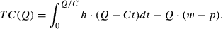
That is, consumers incur holding costs h for each unit of purchased goods. The goods are consumed at rate C; this means that inventory costs decline over time t. Furthermore, consumers must pay Qp for the total purchased quantity of goods. They receive the gross utility of Qw, which is weighed against the purchasing and holding costs. Note that consumers do not pay underage costs, as we assume that they can always purchase on the market at their reservation price.

We divide consumers into two segments: deal‐prone consumers, who are willing to stockpile; and loyal consumers, who value convenience over savings from promotions and thus are not willing to stockpile. We characterize the two different segments by assigning segment‐specific holding costs h ^loyal and h ^dp. Loyal consumers incur high holding costs, which limits their ability to stockpile. Deal‐prone consumers incur lower holding costs and thus are better able to stockpile. We define C ^loyal (resp., C ^dp) as the consumption rate of all consumers in the loyal (resp., deal‐prone) segment.

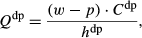
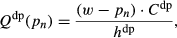
We minimize Equation 1 with respect to Q for both segments. For loyal consumers, holding costs are assumed to be approximately equal to their net utility w − p, ¹ so the unique solution to the cost‐minimization problem for loyal consumers is to set Q ^loyal = C ^loyal. Then loyal consumers purchase the same quantity each period regardless of the retail price, which creates a constant base‐load level of demand—that is, a minimum consumption level without downside variance—for the retail stores.

Low–holding cost (deal‐prone) consumers purchase an optimal quantity Q ^dp such that

Q dp = ( w − p ) · C dp h dp ,

(2)

where, Q ^dp is the optimal order‐up‐to level derived by Blattberg et al. (1981). Deal‐prone consumers purchase during promotions only; they stockpile and demand quantities that depend on the retail price. Retail stores perceive demand from the deal‐prone segment as demand spikes during price promotions.

Focusing on two segments of consumers—one that purchases equal quantities every period and one that purchases only during promotions—is a reasonable approach to modeling demand at the retail level. Each consumer segment exhibits a unique purchasing behavior that requires its own forecasting mechanism. A possible extension would be to consider multiple segments of deal‐prone consumers who differ in terms of their holding costs, however, the mechanics of determining the optimal purchase quantity per segment would not change.

Generalized Household Inventory Model

In the next step, we generalize the household inventory model along two dimensions. We first consider unequal intervals of regular pricing between promotions and then model multiple promotion prices. From the consumer point of view, price promotions should take place approximately when the household inventory approaches zero. Hence, we assume that the corresponding time between promotions is τ* = Q ^dp/C ^dp, where

Q dp = α Q deep dp + ( 1 − α ) · Q shallow dp

.

Let

I n dp ( p n − 1 )

denote consumer inventories at the beginning of the nth promotion, given the retail price p _n−1 at the previous promotion. We assume that deal‐prone consumers have ordered enough to reach their optimal order‐up‐to quantity at promotion n − 1, as described in Equation 2. Inventory at the beginning of the current promotion,

I n dp ( p n − 1 )

, is then calculated as inventory after the previous promotion less consumption over τ _n−1 units of time (recall from section 3.2 that τ _n−1 denotes the actual time interval between promotion n − 1 and promotion n):

I n dp ( p n − 1 ) = [ Q n − 1 dp ( p n − 1 ) − τ n − 1 · C dp ] + .

(3)

Here, we assume that deal‐prone customers first consume all of their existing inventory. If no promotion takes place by the time household inventory reaches zero, then consumers satisfy their current consumption needs via everyday low‐price stores—that is, there is no backlogging. Our assumptions reflect the common retailing practice whereby EDLP prices are higher than promotion prices but lower than regular retail prices. Thus, rational consumers do not stockpile from EDLP purchases and instead wait for the next promotion of a regular retailer (see Iyer and Ye 2000).

Demand from deal‐prone consumers equals the difference between the optimal order‐up‐to level and the consumer inventory level at the beginning of the promotion; at the same time, loyal consumers continue purchasing to accommodate their per‐period consumption. Cumulative demand D _n (p _n ) from both consumer segments during the period of time between the nth promotion and the beginning of the n + 1st promotion is, therefore,

D n ( p n ) = Q n dp ( p n ) − I n dp ( p n − 1 ) + τ n · C loyal if Q n dp ( p n ) ≥ I n ( p n − 1 ) , τ n · C loyal if Q n dp ( p n ) < I n ( p n − 1 ) .

(4)

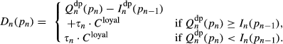
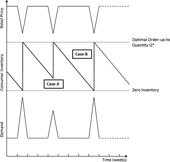
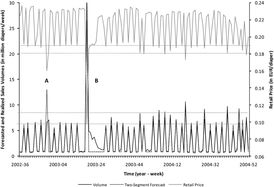
If promotions occur sooner than after τ* units of time then consumers will have leftover inventories, which results in lower demand spikes (see Figure 1, Case A); Mela et al. (1998) observe this effect in an empirical study. If there is no promotion until after τ* units of time have elapsed, then deal‐prone consumers run out of inventory. Yet the absence of backlogging means that demand is lost for the retailer (note that we have not formalized the promotion timing process of the retailer). At the next promotion, deal‐prone consumers purchase enough to reach their optimal order‐up‐to quantity (Figure 1, Case B).

OPEN IN VIEWER

Figure 1

Consumer Inventories When Times between Promotions Are Unequal

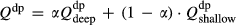
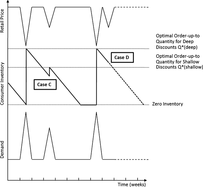
We next consider a scenario involving a regular price point and two promotion price points—namely, prices with deep and shallow discounts. Both of these promotion prices are associated with optimal order‐up‐to levels Q ^dp(·), which follow from Equation 2. These order‐up‐to policies determine the reachable levels of household inventory after the nth promotion:

I n dp ( p n − 1 ) = Q deep dp − τ n − 1 · C dp + = ( w − p deep ) · C dp h dp − τ n − 1 · C dp + if p n − 1 = p deep , Q shallow dp − τ n − 1 · C dp + = ( w − p shallow ) · C dp h dp + α · ( p sh . − p deep ) 2 − τ n − 1 · C dp + if p n − 1 = p shallow .

(5)

In case of a shallow promotion, observe that the opportunity loss (per unit of excess stock) is the holding cost plus forgone savings from being unable to buy at a subsequent deep promotion. A shallow discount following a deep discount has less impact on demand because household inventories are still filled to a fairly high level (see Figure 2, Case C). When a shallow promotion closely follows a deep promotion, the optimal order‐up‐to level for shallow promotions can be lower even than remaining customer inventories. In this case, the shallow promotion has no effect on demand (see Figure 2, Case D).

OPEN IN VIEWER

Figure 2

Linking order‐up‐to Levels, Inventories, and Demand

Two‐Segment Forecasts

Our next step is to use the generalized household inventory model to derive a demand forecast. We first note that demand from loyal consumers is assumed to be constant over time. As shown in section 3.3, loyal consumers demand exactly their consumption rate in every period, hence their demand does not change during promotions. The retailer can easily observe that base–load level of sales during nonpromotion periods and thus has no uncertainty at this point. We, therefore, focus on how the retailer can best forecast demand from deal‐prone consumers during promotions.

By definition, demand from the deal‐prone segment equals the optimal order quantity Q ^dp (given the retail price p _n ) less leftover inventories

I n dp ( p n − 1 )

from the last promotion. That is,

D n ( p n ) = [ Q dp ( p n ) − I n dp ( p n − 1 ) ] + .

(6)

In our setup of the generalized household inventory model, we derived the optimal order‐up‐to level Q ^dp in terms of the current price p _n , inventory holding costs (including opportunity cost), consumers' willingness to pay, and the consumption rate. We treat the last four variables as known parameters of the model, because retailers can estimate them using a regression analysis on historical sales data. Thus, the demand forecasting exercise reduces to a forecast of retail prices for a promotion n and of the household inventory level

I n dp ( p n − 1 )

.

We next formulate a stochastic process that describes the changes in household inventories over time. Household inventories reflect all the relevant information on past promotion prices and on intervals of regular pricing. Let

I n dp

be the aggregated inventory position of consumers at the beginning of the nth promotion. This inventory position depends on the current promotion prices and on the inventory position at the previous promotion; the latter, in turn, depends on the prices of the previous promotion. Because the promotion prices are assumed to follow the random strategy defined previously, we obtain the following stochastic process for the inventory levels:

I n dp ( p n − 1 ) = Q deep dp − τ n − 1 · C dp + with probability α , max [ I n − 1 dp ; Q shallow dp ] − τ n − 1 · C dp + with probability 1 − α .

(7)

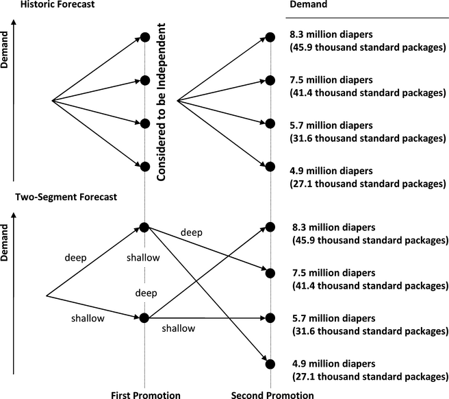
Given the recursive nature of the stochastic process used to describe household inventories, the retailer can “forward calculate” the level of inventory for any upcoming promotion if she knows the history of all previous promotion prices as well as the timing of past and future promotions. All in all, we conclude that if the retailer indeed fixes her promotion schedule in advance, then the set of promotion prices is enough to derive the corresponding demand scenarios at each promotion—that is, by using decision tree logic (see Figure 3). Furthermore, the retailer can sequentially refine her demand forecasts for the promotions that remain in the forecasting period (i.e., after each concluded promotion) by using the realized prices of those promotions. This is a key insight for employing hedging mechanisms: A two‐segment forecast allows hedging to be postponed because the demand forecast improves at the beginning of each promotion within the planning horizon (i.e., it does not worsen over time).

OPEN IN VIEWER

Figure 3

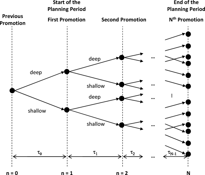
States of the World over Multiple Promotions in Decision Tree Logic

Hedging Demand Scenarios

Even with improved demand forecasting, the retailer still faces uncertainty about demand during promotions. We argue that the retailer can hedge the resulting demand scenarios by using a flexible schedule of supply contracts with the manufacturer. Specifically, we show that a profit‐maximizing retailer should establish a portfolio of forward, spot, and option contracts. To explore this issue formally, we set‐up a model of the supply contracts between a retailer and a manufacturer. In the model setup, we use the result from a companion study (Breiter and Huchzermeier 2014) that a portfolio of flexible contracts can achieve coordination of the supply chain; in particular, the portfolio aligns incentives in a Stackelberg game where the manufacturer is the leader. This result allows us to simplify the model to one that captures two separate optimization problems: one of the retailer and one of the manufacturer.

Supply Contracts

We have outlined how, at each promotion n, a random pricing decision is made. Let z _n denote the state of the world at the beginning of the nth promotion. Each z _n contains the complete retail price path information up to that state at that moment in time. For example, one possible realization of z ₃ could be two shallow promotions in a row followed by a deep discount. Because we assume that both the retailer and the manufacturer know the probability of a shallow or deep discount at each promotion (recall that Pr(p _n  = p _shallow) = 1 − α), they also know the probability of a specific price path at any promotion. We denote this probability as

π z n

.

We now explain the retailer's price‐setting behavior. Let i be the current promotion and let p _i denote the price that the retailer sets for the current promotion. As discussed before, this promotion price is chosen randomly and is therefore unknown to both parties until the promotion begins. For the retailer to remain unpredictable to competitors when choosing the promotion price, she must not consider such parameters as her own inventory or consumers' household inventory. In order to analyze the retailer's behavior across different promotions, we let k < i be the date of some promotion in the past and let j > i be the date of some promotion in the future, where k ∈ {0, 1, ..., N − 1} and j ∈ {1, 2, ..., N}.

The manufacturer offers forward and option contracts at the end of each promotion to receive early orders from the retailer. Forward contracts are commitments of the manufacturer to deliver the quantity of goods at a specified price at a specific future time. The retailer can purchase forward contracts

q i j f ( z i )

at a lead time–dependent forward price f(δ _ij ) per unit, where δ _ij is the lead time between an order at promotion i and delivery at promotion j. We allow for a lead time–dependent discount because earlier commitments entail more operational leverage for the manufacturer. Notation is summarized in Table 1.

OPEN IN VIEWER

Table 1

Parameters of the Retailer and Manufacturer Model

Parameter	Explanation
z n	State of the world—pricing history
p i	Retail price at promotion i
q i j f ( z i )	Quantity of forward contracts purchased
f(δ ij )	Lead time–dependent forward price
q i j r ( z i )	Quantity of option contracts purchased
r(δ ij )	Reservation fee to be paid, when an option is purchased
e(δ ij )	Execution fee to be paid, when an option is executed
q i s ( z i )	Quantity of spot contracts purchased
s i	Spot price
v N	Salvage price
Π r	Retailer profit
I i (z i )	Retailer inventory
h ret.	Holding cost at retail level
G i (z i )	Unserved demand at retail level
g	Goodwill cost per unit not served to consumers
Π m	Manufacturer profit
q i j p ( z i )	Quantity produced
c(δ ij )	Lead time–dependent production cost
J i (z i )	Retailer inventory
h man.	Holding cost at retail level

Like forward contracts, option contracts are a commitment of the manufacturer; but whereas the retailer is required to purchase any goods ordered by means of a forward contract, she has no obligation to execute option contracts. The retailer reserves a quantity

q i j r ( z i )

at a reservation fee r(δ _ij ) per unit. We model European‐type option contracts. These can be executed only at maturity, when the retailer pays the execution fee e(δ _ij ) per unit executed

q i j e ( z j )

. The choice of European‐type option contracts is not restrictive, as the retailer learns about retail prices only shortly before the respective promotion, which is maturity. There is thus no rationale to execute options at another time.

Finally, the retailer can use spot contracts if they are available. Spot quantities

q i s ( z i )

cost s _i per unit. Since the lead time is zero (i.e., δ _ii  = 0), the spot price can exceed the wholesale or forward price. We assume that the spot price is independent of the state of the world, since long‐term price negotiations on contract parameters are standard in the FMCG industry. The prices of all contracts are determined once in the annual buying negotiations and are fixed over the year.

Retailer Model

The retailer's objective is to maximize her cumulated expected profit Π _r , where profit depends on the retailer's pricing decisions and also on uncertain demand. As in the consumer model, we assume that consumers do not backlog; in other words, unmet demand is lost for the retailer (e.g., because consumers purchase at an EDLP store). Lost sales to consumers G _i (z _i ) result in costs g per unit not served.

The FMCG product modeled is not perishable, which allows the retailer to hold inventories at a cost of h ^ret. per unit of the product for one unit of time. Unused inventory is salvaged for a refund v _N at the end of the promotion period. Inventories are built up when forward orders exceed realized demand. In addition to inventories induced by forward purchases, the retailer may choose to build up inventory by executing options or by purchasing products with spot orders. This approach is rational only if, in the following period, flexible sources are limited or expensive enough to outweigh the additional holding costs. Therefore, inventories after a promotion are calculated as inventories after the last promotion in n = i − 1 plus any contracts executed in period i less demand served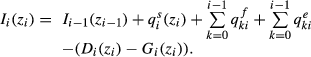

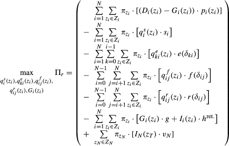
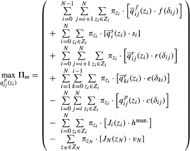
I i ( z i ) = I i − 1 ( z i − 1 ) + q i s ( z i ) + ∑ k = 0 i − 1 q k i f + ∑ k = 0 i − 1 q k i e − ( D i ( z i ) − G i ( z i ) ) .

(8)

The retailer maximizes expected profits over all promotions. Given the structure of available supply contracts, the retailer must determine a profit‐maximizing initial portfolio of contracts as well as an optimal policy for updating this portfolio when new information becomes available. The retailer's objective function over all periods is specified as the sum of profits in all nodes, weighted by the probability of reaching the respective nodes.

We formulate the following stochastic program to maximize retailer profits.

max q i s ( z i ) , q k i e ( z i ) , q i j f ( z i ) , q i j r ( z i ) , G i ( z i ) Π r = ∑ i = 1 N ∑ z i ∈ Z i π z i · ( D i ( z i ) − G i ( z i ) ) · p i ( z i ) − ∑ i = 1 N ∑ z i ∈ Z i π z i · q i s ( z i ) · s i − ∑ i = 1 N ∑ k = 0 i − 1 ∑ z i ∈ Z i π z i · q k i e ( z i ) · e ( δ k i ) − ∑ i = 0 N − 1 ∑ j = i + 1 N ∑ z i ∈ Z i π z i · q i j f ( z i ) · f ( δ i j ) − ∑ i = 0 N − 1 ∑ j = i + 1 N ∑ z i ∈ Z i π z i · q i j r ( z i ) · r ( δ i j ) − ∑ i = 1 N ∑ z i ∈ Z i π z i · G i ( z i ) · g + I i ( z i ) · h ret . + ∑ z N ∈ Z N π z N · I N ( z T ) · v N

subject to: I.

q i j s ( z i ) ≥ 0 , q i j f ( z i ) ≥ 0 , q i j r ( z i ) ≥ 0 , q k i e ( z i ) ≥ 0 , G i ( z i ) ≥ 0 , ∀ i ;

II.

I i ( z i ) = I i − 1 ( z i − 1 ) + q i s ( z i ) + ∑ k = 0 i − 1 q ¯ k i f + ∑ k = 0 i − 1 q k i e ( z i ) − ( D i ( z i ) − G i ( z i ) ) ∀ i ;

III.

I _i (z _i ) ≥ 0 ∀ i;

IV.

G i ( z i ) ≤ D i ( z i ) − q i s ( z i ) − ∑ k = 0 i − 1 q ¯ k i f − ∑ k = 0 i − 1 q k i e ( z i ) ∀ i ;

V.

q k i e ( z i ) ≤ q k i r ∀ i ;

VI.

a a a a a a a a a a

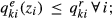
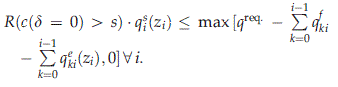
All decision variables must be nonnegative, which is reflected in the first constraint. The second constraint defines inventory, and the third constraint limits inventory to the positive range. Substituting II into III demonstrates that the program requires the retailer either to meet demand or to incur lost sales: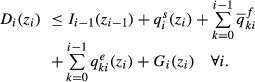

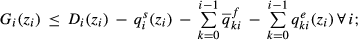
D i ( z i ) ≤ I i − 1 ( z i − 1 ) + q i s ( z i ) + ∑ k = 0 i − 1 q ¯ k i f + ∑ k = 0 i − 1 q k i e ( z i ) + G i ( z i ) ∀ i .

(9)

We argue that lost sales should be optimized as a decision variable because retailers want to maximize store traffic, which drives overall store profit (ECR / Roland Berger Strategy Consultants 2003). Consequently, we require the fourth constraint to define the upper bound for lost sales G _i (z _i ). The fifth constraint ensures that the retailer cannot execute more options than she reserved for that particular time.

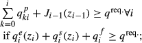
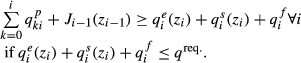
Spot orders are not commitments by the manufacturer, who may simply decline to serve them—as when the cost of short‐term production exceeds the spot or wholesale price. We allow for the possibility that the retailer enforces a required minimum service level q ^req.. The sixth constraint limits retailer orders to the maximum service level agreed by the manufacturer, where R is an indicator function set to 1 when the manufacturer cannot profitably serve spot orders. Note that either spot orders are part of the portfolio or there is no required minimum service level, since spot orders are dominated by options and forwards (Breiter and Huchzermeier 2014). Whether or not there are spot orders is determined in advance by contract parameters. Consequently, the sixth constraint either sets spot orders to zero (for the case of domination) or limits spot orders to the required minimum service level.

The retailer model leads to three cases. In the first case, the retailer orders options and forwards to cover all demand. Then there are no stockouts (contract terms are determined to achieve channel coordination; see Breiter and Huchzermeier 2014). In the second case, the retailer incurs stockouts during this planning period. These stockouts are planned, since contract parameters for forwards and option contracts are determined (i.e., at the beginning of the year) such that channel coordination and a target profit level are achieved. We emphasize that the stochastic programming formulation incorporates a full enumeration of all pricing scenarios and thus includes cases where profitability of the retailer may deviate significantly from the target—for instance, when p _deep is repeatedly “drawn from a fair lottery.” Not accounting for stockouts would be inconsistent with the prices for forwards and option contracts that the manufacturer bids into the market (as a Stackelberg leader). In the third case, the retailer requires a service level above the channel‐coordinating solution (and exerts power in the supply channel). Again the manufacturer determines contract terms. If there is a participation constraint, then he will either exit or serve all orders. Finally stockouts above the required service level are again planned stockouts, although the solution no longer serves to coordinate the channel.

Manufacturer Model

The manufacturer decides on his optimal production schedule and incurs variable costs for each unit produced. Without loss of generality, we normalize fixed costs to zero. Variable costs are likely to depend on lead times. Short lead times create inefficiencies in the channel because the associated overtime charges, additional setup times, and reduced machine utilization rates all increase costs. The manufacturer produces quantities

q i j p ( z i )

at production costs c(δ _ij ) per unit, where δ _ij is the period of time between dates i (when today's order is placed) and j (the delivery date).

The manufacturer has the opportunity to hold inventory at holding costs h ^man.. He faces a trade‐off between producing early under uncertainty at low costs and waiting until uncertainty is resolved, which results in higher production costs. High cost penalties for short‐term production force the manufacturer to consider producing a quantity of the product in advance even under a wholesale price scheme. For this reason, the manufacturer invests in speculative inventories J _i (z _i ). Inventories are built when production for a time i exceeds orders less remaining inventories from the last promotion. The manufacturer salvages excess inventory (i.e., speculative inventories built to serve options and spot orders in peak demand scenarios) for a refund v _N at the end of the planning period. We calculate manufacturer inventory as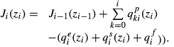

J i ( z i ) = J i − 1 ( z i − 1 ) + ∑ k = 0 i q k i p ( z i ) − ( q i e ( z i ) + q i s ( z i ) + q i f ) .

(10)

The manufacturer determines his production quantities

q i j p ( z i )

knowing that he must serve all options and all forward orders. He can decide not to serve spot orders as long as the retailer does not impose a minimum service level. Recall that we formulated the retailer's optimization program to place spot orders exceeding the required service level only when serving these orders is profitable for the manufacturer. The retailer's decision variables

q ¯ i j f ( z i )

,

q ¯ i j s ( z i )

,

q ¯ i j r ( z i )

and

q ¯ k i e ( z i )

are determined by her own optimization problem, and are therefore exogenous from the manufacturer's perspective. The manufacturer solves his production problem for all reachable states of the world at all promotions within the planning period, which is captured by the following stochastic program.

max q i j p ( z i ) Π m = ∑ i = 0 N − 1 ∑ j = i + 1 N ∑ z i ∈ Z i π z i · q ¯ i j f ( z i ) · f ( δ i j ) + ∑ i = 0 N ∑ z i ∈ Z i π z i · [ q ¯ i s ( z i ) · s i ] + ∑ i = 0 N ∑ j = i + 1 N ∑ z i ∈ Z i π z i · q ¯ i j r ( z i ) · r ( δ i j ) + ∑ i = 1 N ∑ k = 0 i − 1 ∑ z i ∈ Z i π z i · q ¯ k i e ( z i ) · e ( δ k i ) − ∑ i = 0 N ∑ j = i N ∑ z i ∈ Z i π z i · q i j p ( z i ) · c ( δ i j ) − ∑ i = 0 N ∑ z i ∈ Z i π z i · J i ( z i ) · h man . − ∑ z N ∈ Z N π z N · J N ( z N ) · v N

subject to: I.

q i j p ≥ 0 ∀ i ;

II.

J i ( z i ) = J i − 1 ( z i − 1 ) + q k i p − ( q i e ( z i ) + q i s ( z i ) + q i f ) ∀ i ;

III.

∑ k = 0 i q k i p + J i − 1 ( z i − 1 ) ≥ q i e ( z i ) + q i f ∀ i ;

IV(a).

∑ k = 0 i q k i p + J i − 1 ( z i − 1 ) ≥ q req . ∀ i if q i e ( z i ) + q i s ( z i ) + q i f ≥ q req . ;

IV(b).

∑ k = 0 i q k i p + J i − 1 ( z i − 1 ) ≥ q i e ( z i ) + q i s ( z i ) + q i f ∀ i if q i e ( z i ) + q i s ( z i ) + q i f ≤ q req . .

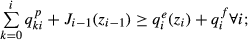
The first constraint limits production quantities to the positive range, and the second constraint defines manufacturer inventories. The third constraint ensures that forward and option orders are always served. The fourth constraint forces the manufacturer to serve demand at least (a) up to the required service level or (b) up to the quantity demanded by the retailer. At each node, either (a) or (b) is active depending on whether or not orders exceed the required service level. The manufacturer may choose to serve more than the required minimum when doing so is profitable. In combination with the third constraint, constraint IVa is extended such that option and forward contracts are served even when they exceed the required minimum service level. The cost of managing and executing portfolios of contracts is viewed—according to our discussions with both retailers and manufacturers—negligible due to the capital‐intensity of promotions and the overall channel benefits—especially when more than one promotion must be planned. Moreover, in practice, subsidies for marketing campaigns paid by the manufacturer often dictate retailers' orders for promoted items. The low profitability of retailers—partly due to the large mismatch costs of such promotion handling—explains their strong interest in more collaborative promotion forecasts.

Application Case Study

Calibration of the Two‐Segment Demand Model

We employ a data set covering diaper sales at a major German supermarket chain (first used by Wiehenbrauk 2010) to calibrate empirically the parameters of the two‐segment demand forecasting model developed in the previous section. Diapers are an important fast‐moving consumer good for the industry because they generate traffic and account for a large fraction of store sales (Huchzermeier et al. 2002). Also the diapers industry is characterized by constant end consumer demand and long innovation cycles. It is thus expected that customers will adjust their shopping behavior in response to prices set by the retailer. Diapers exhibit a highly characteristic demand pattern that features strong demand spikes during promotions. Furthermore, although retail prices of diapers have decreased significantly in recent years, diapers remain one of the more expensive FMCG items. Past research has shown that some consumers make price‐conscious purchase decisions that result in stockpiling behavior during promotions (Huchzermeier et al. 2002, Wiehenbrauk 2010). We, therefore, expect that our results are generalizable to other kinds of fast‐moving consumer goods that induce a strong consumer response to price promotions.

The data set contains weekly sales volumes and retail prices of the Pampers Baby Dry brand over a period of 121 weeks from the middle of 2002 to the end of 2004. We provide volumes in statistical units (standard packages) of 180 diapers each, which is the industry's standard and corresponds approximately to a popular package size. To simplify the interpretation of our analysis, we also recalculate prices and volumes on a per‐diaper basis. The regular price of a diaper in our data set is about 0.23 euro each (on average, 41.14 euro per standard package). There are typically 2 weeks of regular pricing between promotions, which at this supermarket chain are thus quite frequent and usually last for 1 week. The retailer distributes promotion catalogs to households the weekend before a promotion starts and maintains the catalog prices during the following week. Over the period of time analyzed, there were two exceptionally deep promotions, during which retail prices dropped to 0.16 and 0.10 euro per diaper. In weeks 50/2002 to 51/2002, an extremely deep promotion over 2 weeks occurred (promotion A in Figure 4; demand was filled in 2 weeks instead of 1). In weeks 19/2003 to 24/2003, another extreme discount influenced consumers' behavior (promotion B in Figure 4). The latter was a one‐time two‐for‐one offer to promote the new Pampers (Skarka 2003). Overall, sales in terms of both units and revenues show a characteristic promotion pattern.

OPEN IN VIEWER

Figure 4

Forecast and Realized Sales Volumes of Pampers Baby Dry at the Retail Chain (Source: Sales Volumes and Prices Based on Wiehenbrauk 2010; Forecast Based on Own Calculations; Compare Breiter and Huchzermeier 2010)

We refer to our discussion of the two‐segment forecast and use Equations 6 and 4 to derive the following model for calibration: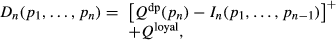

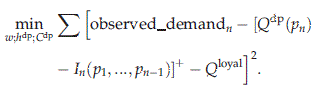
D n ( p 1 , … , p n ) = Q dp ( p n ) − I n ( p 1 , … , p n − 1 ) + + Q loyal ,

(11)

where

Q dp ( p n ) = ( w − p n ) · C dp h dp ,

(12)

I n ( p 1 , … , p n − 1 ) = [ max [ I n − 1 dp ( p 1 , … , p n − 2 ) ; Q dp ( p n − 1 ) ] − τ n − 1 C dp ] + .

(13)

Therefore, our empirical minimization problem is now

a a a a a a a a a a a a a a

(14)

This model estimates demand during a promotion based on the current and last periods' retail prices. We minimize quadratic deviations of forecasted demand from realized demand. The program is nonlinear and requires a search algorithm to reach the global optimum. So that we may calibrate the model to the more common retail price range, we leave out the two extreme promotions (mentioned in our initial analysis) to avoid overfitting. ² We thereby utilize accurate predictors for simulating shallow and deep promotions in the numerical study. In total, we use 113 out of 121 weeks of data when calibrating the model.

We use data from the retail data set to calibrate values of the consumption rates C for both the loyal and the deal‐prone consumer segments and also to calibrate values of household inventory holding costs h and the reservation price w for deal‐prone consumers. In our theoretical model of household behavior, we assumed that the retailer can infer these values and thus can use them to forecast demand. Therefore, in order to conduct a numerical study of the proposed demand forecasting model when flexible contract portfolios are added, we must first estimate these parameters from the available retail data set.

We derive a consumption rate of approximately 2.5 million diapers (about 13,800 standard packages) per week for the deal‐prone segment (note that the supermarket chain data cover sales in the chain's stores throughout Germany). The loyal segment consumes, on average, some 0.9 million diapers (about 4800 standard packages) per week. The deal‐prone segment appears to be at least twice as large as the loyal consumer segment if we assume that the actual consumption per consumer is similar across segments. The estimate of deal‐prone consumers' holding costs is 0.01 euro per diaper per week (2.06 euro per standard package). This equals about 5% of their reservation price for this product, which is estimated to be 0.22 euro per diaper per week (38.90 euro per standard package). This reservation price makes sense for the deal‐prone segment, since it lies below the regular retail price. We omit opportunity cost because the data show that consumers during shallow promotions purchase only enough to cover their consumption until the next promotion—a result of the retailer's policy of regular promotions. The fitted model explains R ² = 0.951 of all variability of sales in the 113 weeks of data considered (R ² = 0.891 when considering all 121 data–points). The mean absolute percentage error (MAPE) is 15.9% ³ . Figure 4 shows retail prices, forecasts, and realized demand over the full 121 weeks of data available.

Finally, we show that a simplified model working with only one price each for shallow and deep promotions is able to generate a good forecast. In the data, shallow promotion prices average about 0.19 euro per diaper (34.18 euro per standard package). Nearly a fourth of all promotions at the chain are deep promotions, during which diapers sell for about 0.18 euro each (on average, 32.04 euro per standard package). Figure 4 uses dotted lines to mark these two price levels and the corresponding order‐up‐to levels. The restricted model with only two promotion prices still explains R ² = 0.760 of all variability in sales over the 113 weeks of data considered, and the mean absolute percentage error is 19.6%. Table 2 summarizes the calibrated parameters that will be used in the numerical study.

OPEN IN VIEWER

Table 2

Parameters Calibrated for the Numerical Study

	Explanation
Observed parameters
p shallow = 0.19 euro/diaper (34.18 euro/package)	Retail price for shallow discounts
p deep = 0.18 euro/diaper (32.04 euro/package)	Retail price for deep discounts
π shallow = 0.75	Probability of a shallow promotion
π deep = 0.25	Probability of a deep promotion
Estimated parameters
c dp = 2.5 million diapers/week (13,800 packages)	Consumption rate of the deal‐prone consumer segment
h dp = 0.01 euro/diaper (2.06 euro/package)	Holding costs of deal‐prone consumers
w = 0.22 euro/diaper (38.90 euro/package)	Reservation price of deal‐prone consumers

Forecasting is a trade‐off between the costs of gathering information and the accuracy achieved. Incorporating brand‐ and store‐switching behavior would require that we collect real‐time data on the pricing of all the retailer's competitors and on all brand substitutes. Given the very good fit of the simpler model already presented, that much effort cannot be justified for the diapers category at the retail chain in question. Using retailer inventory data would allow the model to incorporate stockouts. A stockout at the retailer level may well have occurred during promotion A, for which the estimate is far greater than the actual quantity sold and after which consumers continue purchasing at a shallower discount. Since we excluded this promotion when fitting and since we see no evidence of other stockouts, we believe that a nontruncated fitting model is optimal for this data set.

Hedging Demand for a Multi‐Promotion Campaign

Here, we show the potential impact of two‐segment forecasts and portfolios of hedging supply contracts in a business case based on the parameter values estimated in the previous section and on the optimization programs of both retailer and manufacturer.

Consider a planning period that contains two promotions, and consider the possible demand realizations for the second promotion. As we argued in presenting the theoretical model, there are four possible retail pricing paths in a game with two promotions: shallow‐shallow, deep‐deep, deep‐shallow, and shallow‐deep. Hence, there are four possible realizations of demand (see Figure 5 for the discrete distribution of demand). We use the recursive demand forecasting equation from section 4, to calculate these four values as follows.

OPEN IN VIEWER

Figure 5

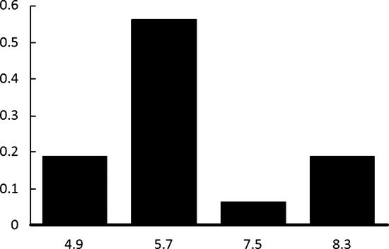
Distribution of Demand for Two Promotion Prices

A deep discount after a shallow discount: 8.3 million diapers (45,900 standard packages)

A deep discount after a deep discount: 7.5 million diapers (41,400 standard packages)

A shallow discount after a shallow discount: 5.7 million diapers (31,600 standard packages)

A shallow discount after a deep discount: 4.9 million diapers (27,100 standard packages)

That demand is path‐dependent on retail prices is key in the forecasting analysis, but this fact is often disregarded in practice. However, the structure of demand risk in the presence of stockpiling consumers shows that promotions cannot be evaluated independently (see Figure 6).

OPEN IN VIEWER

Figure 6

Structure of Demand Risk under the Historical Forecast and under the Two‐Segment Forecast

When there are two promotions within the planning period, the retailer optimally orders products from the manufacturer at three moments in time: (i) after the promotion price of the preceding promotion is known (at n = 0, before the beginning of the planning period), (ii) after the promotion price of the first promotion is known (i.e., at n = 1), and (iii) after the promotion price of the second promotion is known (i.e., at n = 2).

Suppose that promotions recur every 3 weeks and that production costs depend on lead times. We assume that producing with only 3 weeks of lead time is 10% more expensive for the manufacturer than producing with a lead time of 6 weeks, so short‐term production is 20% more expensive than long‐term production. We assume that the short‐term production costs for zero lead time exceed the wholesale price and set c _{zero lead time} = 0.17 euro per diaper (30.0 euro per standard package). Thus we exclude the trivial case of profitable short‐term production in which the manufacturer serves all instant orders. ⁴

We assume that the retailer and the manufacturer incur equal per‐period holding costs of h = 0.03 euro per diaper (5.0 euro per standard package). We assume that the promotion items modeled are “outdated” after the 6‐week promotion cycle (e.g., a new packaging is used or a new toy is included in promotion items). Nevertheless, we assume that the manufacturer can find a last‐minute buyer to salvage leftover goods at a loss for v _m  = 0.09 euro per diaper (16 euro per standard package) at the end of the planning cycle. If the retailer cannot serve demand, then she must invest in winning consumers back; for this, we assume goodwill costs of g _r =0.06 euro per diaper (10 euro per standard package). Table 3 summarizes the parameter values that are not observable and so are based on assumptions for this numerical study.

OPEN IN VIEWER

Table 3

Parameter Choices for the Numerical Study

Parameters	Explanation
c zero lead time = 0.17 euro/diaper (30.0 euro/package)	Short‐term production costs (no lead time)
c one period = 0.15 euro/diaper (27.5 euro/package)	Medium‐term production costs (3 weeks)
c two periods = 0.14 euro/diaper (25.0 euro/package)	Long‐term production costs (6 weeks)
h = 0.03 euro/diaper (5.0 euro/package)	Holding and handling costs per unit of inventory
g r  = 0.06 euro/diaper (10.0 euro/package)	Costs of goodwill for demand not served
v m  = 0.09 euro/diaper (16.0 euro/package)	Salvage value for the manufacturer
v r  = 0.00 euro/diaper	Salvage value for the retailer

As stated before, a principal limitation is that the retailer and the manufacturer agree on the wholesale price in a yearly negotiation. This means that the wholesale price is fixed and cannot be changed by either party. By European law, retailers cannot sell below cost. It is, therefore, always profitable for the retailer to serve all demand, so she would like to achieve a 100% service level. In the example just described, short‐term production costs do not reach the retail price in any state of the world. Hence, short‐term production is profitable from a channel perspective, for otherwise it would not be employed. We allow for a spot price below short‐term production cost. In this case, the manufacturer can maximize his profits by allowing for stockouts, that is, he does not use short‐term production to serve spot orders (or does so only up to an existing minimum service level). The supply chain then fails to achieve coordination because of double marginalization: supply chain profits are maximized when all demand is served, but the manufacturer does not provide sufficient supply. The retailer would like to order sufficient spot contracts to serve all demand, so her purchasing decision naturally maximizes supply chain profits. Note that, in contrast to other coordination models, the production decision must be coordinated whereas the purchasing decision is optimal.

Retailers often do not confirm their orders until shortly before delivery is due. The result is waste in the supply chain, which we aim to demonstrate by way of an initial simulation of a retailer who orders on a spot contract basis only. In other words, the retailer orders the demand observed via spot orders. We assume that a powerful retailer puts pressure on the wholesale price; Hasse (2010), for example, reports that retailer power in Germany results in low margins at the manufacturer level. A wholesale price of 0.15 euro per diaper (25.0 euro per standard package) reduces manufacturer profits to zero under a 81% required service level. ⁵ Therefore, the manufacturer serves retailer orders in all cases except for a deep discount after a shallow discount. In the case of a stockout, the loss is 0.8 million diapers (4500 standard packages). The manufacturer splits production between orders placed with a long lead time and those placed at the last minute (see Table 4 for the corresponding production decisions under a wholesale price scheme). Because a historical forecast is employed, long–lead time production quantities are equal in both periods. The manufacturer employs short‐term production to serve all orders until the required service level is exhausted. An integrated firm would serve all demand in all states—given that the retail price exceeds the short‐term production costs—and thereby achieve an integrated channel profit of 461,000 euro. The uncoordinated supply chain reaches 95% of the possible channel profits. ⁶

OPEN IN VIEWER

Table 4

Optimal Production and Order Policies

Time	Case	Order decision (in standard packages)	Production decision (in standard packages)
Wholesale price scheme without two‐segment forecast
n = 0		No orders	Produce 31,600 units for t 1, 31,600 units for t 2
n = 1	p 1 = deep	Order 45,900 spot contracts	Produce 9800 units for t 1, stockout of 4500 units
n = 1	p 1 = shallow	Order 31,600 spot contracts	Serve all orders
n = 2	p 1 = deep and p 2 = deep	Order 41,400 spot contracts	Produce 9800 units for t 2, serve all demand
n = 2	p 1 = deep and p 2 = shallow	Order 27,100 spot contracts	Serve all demand, salvage 4500 units
n = 2	p 1 = shallow and p 2 = deep	Order 45,900 spot contracts	Produce 9800 units for t 2, stockout of 4500 units
n = 2	p 1 = shallow and p 2 = shallow	Order 31,600 spot contracts	Serve all demand
Optimal production policy under a two‐segment forecast (changes compared to the base case in parentheses)
n = 0		No orders	Produce 31,600 units for t 1, 27,100 units for t 2 (−4500 units)
n = 1	p 1 = deep	Order 45,900 spot contracts	Produce 9800 units for t 1, stockout of 4500 units
n = 1	p 1 = shallow	Order 31,600 spot contracts	Produce 4500 units for t 2 (+4500 units)
n = 2	p 1 = deep and p 2 = deep	Order 41,400 spot contracts	Produce 14,300 units for t 2 (+4500 units), serve all demand
n = 2	p 1 = deep and p 2 = shallow	Order 27,100 spot contracts	Serve all demand, salvage no units (−4500 units)
n = 2	p 1 = shallow and p 2 = deep	Order 45,900 units with spot contracts	Produce 9800 units for t 2, stockout of 4500 units
n = 2	p 1 = shallow and p 2 = shallow	Order 31,600 standard packages with spot contracts	Serve all demand
Option, forward, and spot contracts under two‐segment forecasting
t 0		Reserve 14,300 options for t 1, buy 31,600 forward contracts for t 1	Produce 31,600 units for t 1, 27,100 units for t 2
t 1	p 1 = deep	Reserve 14,300 options for t 2, buy 27,100 forward contracts for t 2, execute 14,300 options	Produce 14,300 units for t 1, serve all demand (45,900 units)
t 1	p 1 = shallow	Reserve 14,300 options for t 2, buy 31,600 forward contracts for t 2, execute no options	Produce 4500 units for t 2, serve all demand (31,600 units)
t 2	p 1 = deep and p 2 = deep	Execute 14,300 options	Produce 14,300 units for t 2, serve all demand (41,400 units)
t 2	p 1 = deep and p 2 = shallow	Execute no options	No production, serve all demand (27,100 units)
t 2	p 1 = shallow and p 2 = deep	Execute 14,300 options	Produce 14,300 units for t 2, serve all demand (45,900 units)
t 2	p 1 = shallow and p 2 = shallow	Execute no options	No production, serve all demand (31,600 units)

A two‐segment forecast is beneficial in that the manufacturer can postpone part of his long‐term production decision at n = 0 until he receives additional information from the first promotion at n = 1 (see Table 4). He produces a lower amount with his long‐term technology at n = 0 for the second promotion at n = 2 and, when the discount for the first promotion at n = 1 is only shallow, he produces an additional quantity at n = 2. The manufacturer can thus eliminate excess inventories for the second promotion at n = 2. The effect of introducing a two‐segment forecast depends strongly on the form of the lead time–dependent production cost function. Under linear production cost discounts, supply chain profits increase by 3000 euro. The manufacturer postpones part of his long‐term production decision, and the savings on holding costs are balanced by increased production costs. The effect of two‐segment forecasts is stronger for convex production cost functions.

The two‐segment forecast reduces but does not eliminate risk. To share the remaining risk between retailer and manufacturer, we employ option contracts with maturity one period after the purchase date. In particular, the retailer can purchase options at n = 0 for execution at the first promotion at n = 1 and then purchase options at n = 1 for execution at the second promotion at n = 2. This limited offer of option contracts is sufficient to achieve coordination under a Pareto improvement constraint in the setting described—namely, when demand is served in all states of the world.

We set the execution fee at the marginal production cost in order to avoid renegotiation. Then the reservation fee determines the allocation of both risk and profits between the two supply chain parties. The manufacturer receives zero profits when the reservation fee is lowered to 0.01 euro per diaper (1.40 euro per standard package), which represents the lower bound on the set of Pareto‐improving prices. The upper bound on this Pareto set is driven by the retailer's profit function. The retailer requires at least the profit earned in the status quo; in other words, she requires a reservation fee of 1.55 euro per standard package (or lower) to participate.

Given this set of option parameters, the retailer will purchase sufficient options to cover demand in all states (see Table 4); that is, the supply chain reaches “zero lost sales.” The manufacturer is willing to accept the resulting 100% service level because he receives the reservation fee in all states of the world. At the same time, the retailer avoids carrying inventory because option contracts provide the necessary flexibility, achieving “zero excess inventories.” Supply chain profits in this case increase by 26,000 euro to 464,000 euro. Two factors account for this gain: first, the retailer saves goodwill costs because a higher service level is achieved; second, the supply chain earns profits from the additional units sold to consumers.

Our assumption that the transportation component of the manufacturer's costs depends on the lead time between commitment and latest delivery (cf. Cachon 2004) has the effect of reducing the cost of serving forward orders. Again, we find a Pareto set of contract parameters that achieve an increase in profits for both players. The retailer does not accept forward contracts when the forward price exceeds the sum of the reservation fee and the execution fee, which comes to 0.15 euro per diaper (26.48 euro per standard package). The lower boundary is again defined by the manufacturer's Pareto improvement constraint. We assume that each unit ordered under a forward scheme saves 0.003 euro per diaper (0.50 euro per standard package, or 2% of long‐term production costs) in transportation costs. In this case, the manufacturer requires a forward price of at least 0.14 euro per diaper (25.98 euro per standard package).

The retailer takes advantage of the two‐segment forecast and places additional forward orders after a shallow promotion. Deal‐prone consumers will have little leftover inventory at the next promotion, and demand will be relatively high. Table 4 shows the order decisions of the retailer as well as the production decisions of the manufacturer when there are both forward and option contracts.

We find that wholesale price contracts alone do not achieve coordination, which leads us to discuss three levers for improvement. First, two‐segment forecasts reduce inventory requirements at the manufacturer level. Second, option contracts achieve coordination and Pareto improvement. Third, forward contracts reduce the costs of serving an order, and therefore enable additional profits for both parties. Figure 7 shows that supply chain profits can be increased by 13% if there is a 81% initial service level in the business case discussed.

OPEN IN VIEWER

Figure 7

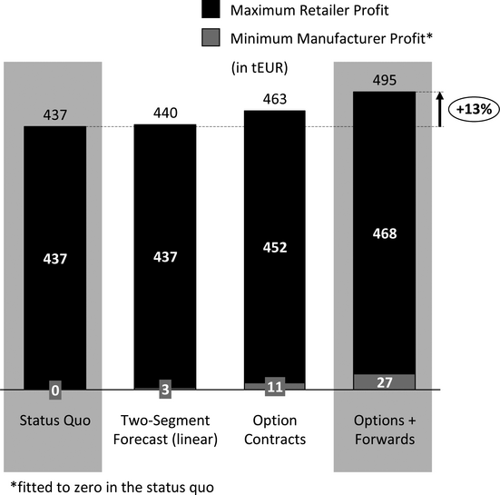
Profits in the Status Quo and under a Portfolio of Hedging Contracts (Compare Breiter and Huchzermeier 2010)

Conclusion

This article answers the question of how to deal optimally with the demand risk induced by price promotions in the fast‐moving consumer goods industry. The approach chosen combines improved forecasting mechanisms and coordinating contracts. Unlike earlier work, this study considers multiple price discounts within the planning period. Employing a combination of flexible (spot), semiflexible (option), and inflexible (forward) contracts requires that the retailer plans beyond the next promotion. We derive two key insights: the retailer should take into account pricing paths and model promotions as interdependent events; and portfolios of coordinating contracts can improve service levels and mitigate excess inventory.

Managers in the FMCG industry should not treat promotional demand as being independently and identically distributed. The two‐segment forecast shows that demand during price promotions depends strongly on household inventory levels. Therefore, demand is path dependent and so each promotion has an impact on subsequent promotions. Forecasting multiple promotions is easier than forecasting a single promotion, since each promotion provides an information update on the realized promotion price that helps to predict demand during the following promotion(s).

We show that simultaneously achieving zero excess inventories and zero lost sales is possible via the combination of a two‐segment forecast and a portfolio of hedging supply contracts. Note that this study includes both the case of channel coordination (i.e., “grow the pie”) and the case of retail power that forces service levels to be much higher (e.g., to the point of no participation by the manufacturer). In short, a portfolio of forward and option contracts can distribute inventory arbitrarily in the supply chain while achieving either channel coordination or “exceptional” service levels—even for peak demand scenarios. Moreover, excess inventories at the retailer level can be entirely eliminated at (any or only) the last promotion.

Our numerical study, which is based on the German diapers industry, shows that neither push nor pull wholesale price contracts maximize supply chain profits. In the status quo, supply chain partners fail to “maximize the pie” (the distributable profits). A portfolio of contracts allows arbitrary risk sharing; it thereby enables Pareto improvement in terms of individual profits and, simultaneously, channel coordination in terms of supply chain profits. If short‐term production is possible, then service levels can reach 100% under coordination even when the cost of short‐term production exceeds the spot price. This would not be possible under a single wholesale price; in that case, the manufacturer would have no incentive to offer such a service level because he incurs a loss on every unit produced short term to serve spot orders.

We conclude this study with a note on our assessment of whether the system developed can be easily implemented in the FMCG industry. Two‐segment forecasts do not require any data that are not already known to the retailer. Supply options are closely related to buyback contracts, which are well known to the FMCG industry. It is, therefore, reasonable to suppose that option contracts would be accepted by the industry. Option contracts are superior to buyback contracts in the context of this industry because the former can be hedged by short‐term production.

Given that the first‐best solution is reached, service levels would no longer be an issue in retailer–manufacturer relations in the FMCG industry. Negotiations in the industry could remain competitive, but they need not be hostile because in this case, cost recovery (remuneration for supply chain inefficiencies or increased agency costs) is not necessary. Our study thus shows that achieving a win–win situation is possible. Consequently, implementing the approach presented here is in the best interest of both supply chain parties.

Footnotes

Acknowledgment

This research received the Science Award 2013 of GS1 Germany and the European Retail Institute; the second author acknowledges the financial support.

1

This assumption is without loss of generality. Alternatively, we could assume that holding costs are at least equal to the net utility, while assuming that consumers do not purchase less than the per‐period consumption rate.

2

Including the two extreme promotions increases the consumption rate of the loyal segment by 12%, a result that suggests these promotions attracted consumers from outside the system.

3

To test the quality of the model, we additionally fit across the first 50% of data, excluding the extreme promotions, and then calculate the quality of fit on the second 50% of data–points: R ² = 0.938, MAPE = 20.1%.

4

In that case the manufacturer could profitably serve unlimited demand by producing short term, but this is not realistic. So here, the first‐best solution would be reached even under a wholesale price scheme.

5

That is, the retailer serves all demand in 81% of all states of the world.

6

Supply chain efficiency decreases to 82% of profits when no required minimum service level can be enforced. Our assumption of a minimum required service level thus reduces the need for coordination.

References

1.

Arminger G. 2008. Forecast Sharing and CPFR Implementation. Presentation at the Progressive Management Program (PMP) of ECR Europe at WHU—Otto Beisheim School of Management.

Go to Reference

2.

Bandyopadhyay S. Paul A. A. . 2010. Equilibrium returns policies in the presence of supplier competition. Market. Sci. 29(5): 846–857.

Go to Reference

3.

Bell D. R. Hilber C. A. L. . 2006. An empirical test of the theory of sales: Do household storage constraints affect consumer and store behavior? Quant. Market. Econ. 4(2): 87–117.

Go to Reference

4.

Bell D. R. Chiang J. Padmanabhan V. . 1999. The decomposition of promotional response: An empirical generalization. Market. Sci. 18(4): 504–526.

+ Show References

5.

Bell D. R. Iyer G. Padmanabhan V. 2002. Price competition under stockpiling and flexible consumption. J. Market. Res. August: 292–303.

+ Show References

6.

Blattberg R. C. Eppen G. D. Lieberman J. . 1981. A theoretical and empirical evaluation of price deals for consumer nondurables. J. Market. 45(1): 116–129.

+ Show References

7.

Blattberg R. C. Briesch R. Fox E. J. . 1995. How promotions work. Market. Sci. 14(3): 122–132.

Go to Reference

8.

Breiter A. Huchzermeier A. . 2010. The new logic of truly efficient retail promotions. Int. Commerce Rev. 9(1): 36–47.

+ Show References

9.

Breiter A. Huchzermeier A. . 2014. Portfolios of coordinating contracts when retailers possess channel power. Working paper, WHU—Otto Beisheim School of Management, Vallendar, Germany.

+ Show References

10.

Burnetas A. Ritchken P. . 2005. Option pricing with downward‐sloping demand curves: The case of supply chain options. Manage. Sci. 51(4): 566–580.

Go to Reference

11.

Cachon G. P. 2004. The allocation of inventory risk in a supply chain: Push, pull, and advance‐purchase discount contracts. Manage. Sci. 50(2): 222–238.

+ Show References

12.

Cachon G. P. Kök A. G. . 2010. Competing manufacturers in a retail supply chain: On contractual form and coordination. Manage. Sci. 56(3): 571–589.

Go to Reference

13.

Chandon P. Wansink B. . 2002. When are stockpiled products consumed faster? A convenience–salience framework of postpurchase consumption incidence and quantity. J. Market. Res. 39(3): 321–335.

Go to Reference

14.

Dong L. Zhu K. . 2007. Two‐wholesale‐price contracts: Push, pull, and advance‐purchase discount contracts. Manuf. Serv. Oper. Manag. 9(3): 291.

Go to Reference

15.

ECR / Roland Berger Strategy Consultants . 2003. Optimal shelf availability—increasing shopper satisfaction at the moment of truth. ECR.

Go to Reference

16.

ECR Australia . 2010. Winning with promotions industry report.

+ Show References

17.

Gupta S. 1988. Impact of sales promotions on when, what, and how much to buy. J. Market. Res. 25(4): 342–355.

+ Show References

18.

Hasse S. 2010. Handelsmacht macht Sorgen (Retailer power creates concerns). Lebensmittel Zeitung. July 1 News.

Go to Reference

19.

Hendel I. Nevo A. . 2006a. Measuring the implications of sales and consumer inventory behavior. Econometrica 74(6): 1637–1673.

+ Show References

20.

Hendel I. Nevo A. . 2006b. Sales and consumer inventory. Rand J. Econ. 37(3): 543–561.

Go to Reference

21.

Hopp A. 2008. Collaboration approaches at Metro. Presentation at the Progressive Management Program (PMP) of ECR Europe at WHU—Otto Beisheim School of Management.

Go to Reference

22.

Hua X. 2011. Future ECR initiatives. Operating Board Meeting of ECR Europe. Brussels, May 9.

Go to Reference

23.

Huchzermeier A. Iyer A. . 2010. Supply chain management in a promotional environment. Krafft M. Mantrala M. K. , eds. Retailing in the 21st Century ‐ Current and Future Trends. Springer Verlag, Berlin‐Heidelberg, Germany.

Go to Reference

24.

Huchzermeier A. Iyer A. Freiheit J. . 2002. The supply chain impact of smart customers in a promotional environment. Manuf. Serv. Oper. Manag. 4(3): 228–240.

+ Show References

25.

Iyer A. Ye J. . 2000. Assessing the value of information sharing in a promotional retail environment. Manuf. Serv. Oper. Manag. 2(2): 128.

+ Show References

26.

Jeuland A. P. Narasimhan C. . 1985. Dealing temporary price cuts by seller as a buyer discrimination mechanism. J. Bus. 58(3): 295–308.

Go to Reference

27.

Jeuland A. P. Shugan S. M. . 1983. Managing channel profits. Market. Sci. 2(3): 239–272.

Go to Reference

28.

Lal R. Little J. D. C. Villas‐Boas J. M. . 1996. A theory of forward buying, merchandising, and trade deals. Market. Sci. 15(1): 21–37.

+ Show References

29.

Lariviere M. A. Porteus E. L. . 2001. Selling to the Newsvendor: An analysis of price‐only contracts. Manuf. Serv. Oper. Manag. 3(4): 293.

Go to Reference

30.

Martinez‐de Albéniz V. Simchi‐Levi D. . 2005. A portfolio approach to procurement contracts. Prod. Oper. Manag. 14(1): 90–114.

Go to Reference

31.

McCardle K. Rajaram K. Tang C. S. . 2004. Advance booking discount programs under retail competition. Manage. Sci. 50(5): 701–708.

Go to Reference

32.

Mela C. F. Jedidi K. Bowman D. . 1998. The long‐term impact of promotions on consumer stockpiling behavior. J. Market. Res. 35(2): 250–262.

+ Show References

33.

Mundt A. 2010. Interview. Lebensmittel Zeitung. September 24 Journal.

+ Show References

34.

Özer O. Uncu O. Wei W. . 2007. Selling to the Newsvendor with a forecast update: Analysis of a dual purchase contract. Eur. J. Oper. Res. 182 (3): 1150–1176.

Go to Reference

35.

Perakis G. Zaretsky M. . 2008. Multiperiod models with capacities in competitive supply chain. Prod. Oper. Manag. 17(4): 439–454.

Go to Reference

36.

Pesendorfer M. 2002. Retail sales: A study of pricing behavior in supermarkets. J. Bus. 75(1): 33–66.

Go to Reference

37.

Ramesh R. V. 2010. Lot‐sizing decisions under limited‐time price incentives: A review. Omega 38(3–4): 118–135.

Go to Reference

38.

Rotemberg J. J. 2005. Customer anger at price increases, changes in the frequency of price adjustment and monetary policy. J. Monetary Econ. 52(4): 829–852.

Go to Reference

39.

Rück D. 2010. Mehr Effizienz für Handzettelwerbung (More efficiency for leaflet advertisement). Lebensmittel Zeitung. February 26 Marketing News.

Go to Reference

40.

Salop S. Stiglitz J. E. . 1982. The theory of sales: A simple model of equilibrium price dispersion with identical agents. Am. Econ. Rev. 72(5): 1121–1130.

Go to Reference

41.

Simon H. Fassnacht M. . 2009. Preismanagement (Price Management). Gabler, Wiesbaden, Germany.

Go to Reference

42.

Skarka C. 2003. Procter startet Attacke mit Pampers (Procter starts attack with pampers). Lebensmittel Zeitung. May 15 Top News.

Go to Reference

43.

Spinler S. Huchzermeier A. Kleindorfer P. . 2003. Risk hedging via options contracts for physical delivery. OR Spectrum 25(3): 379–395.

Go to Reference

44.

Srinivasan S. Pauwels K. Hanssens D. M. Dekimpe M. G. . 2004. Do promotions benefit manufacturers, retailers, or both? Manage. Sci. 50: 617–629.

Go to Reference

45.

Tang C. S. Rajaram K. Alptekinoğlu A. Ou J. . 2004. The benefits of advance booking discount programs: Model and analysis. Manage. Sci. 50(4): 465–478.

Go to Reference

46.

Varian H. R. 1980. A model of sales. Am. Econ. Rev. 70(4): 651–659.

+ Show References

47.

Wiehenbrauk D. 2010. Collaborative Promotions ‐ The Value of Upstream Information Sharing. Springer Verlag, Heidelberg, Germany.

+ Show References