
Abstract
In this study, we consider a supplier's contract offerings to a buyer who may obtain improved forecasts for her demand over time. We investigate how the supplier can take advantage of the buyer's better forecasts and what kind of contracts he should offer to the buyer in order to maximize his profits. We model a natural forecast evolution where the buyer can obtain a more accurate forecast closer to the selling season. We assume there is information asymmetry between the buyer and the supplier at all times in that the buyer understands her demand better than the supplier. Three types of contracts that the supplier can offer are considered: (1) one where a contract is offered before the buyer has a chance to obtain improved forecasts, (2) one where a contract is offered after the buyer has obtained improved forecasts, and (3) a contingent (dynamic) contract which offers an initial contract to the buyer before she obtains improved forecasts, followed by a later contract (contingent on the initial contract) offered after improved forecasts have been obtained. We consider two scenarios: (1) where the supplier is certain that the buyer can obtain more accurate forecasts over time, and (2) where the supplier is uncertain about the buyer's forecasting capability (or forecasting cost). In the first scenario, we show that among the three types of contracts, the contingent contract is always the most profitable for the supplier. Furthermore, using the contingent contract, the supplier always benefits from higher accuracy of the buyer's demand forecasts. In the second scenario, we explicitly model the supplier's level of certainty about the buyer's capability of obtaining better forecasts, and explore how the supplier can design contracts to induce the buyer to obtain better forecasts when she is capable.
Introduction
The effect of a buyer's forecast accuracy on supply chain profits has drawn a lot of attention recently. It is intuitive to expect that both supplier and buyer would benefit from better demand information. However, under information asymmetry and certain types of contract structures, it may not be true that both parties would benefit from improved demand information. Previous literature (e.g., Taylor 2006) showed that the supplier may prefer to contract with the buyer before more accurate demand information is received. We note however that such a result was obtained under the assumption that the buyer receives only one forecast and the supplier utilizes static contracts, where contract ordering takes place only once in a procurement season. In this study, we consider a two‐period model where a supplier sells goods to a buyer under information asymmetry and multiple demand forecasts before the selling season. We assume that the buyer, due to her proximity to the markets in which she is selling, may have better demand information than the supplier does. Furthermore, as the selling period approaches, the buyer may have the capability to obtain even better (more accurate) forecasts. We focus on investigating when the buyer would have the incentive to obtain better forecasts, and what kind of contract offerings would allow the supplier to benefit from the better information obtained by the buyer over the procurement season. In addition to static contracts, we consider another type of contract (contingent contract) which allows multiple ordering opportunities, and show that such a contract can guarantee that the supplier always benefits from the buyer's improved demand information. Recently, we have worked with a major Tier 1 auto parts supplier who uses a contingent contract, as considered in our study, to sell to aftermarket parts retailers. The retailers are given a menu of prices and quantities to choose from initially. At a later date, when the retailers have better information on their demand, they can order more (at a higher unit price than the original order) or decrease their order and get some money back (at a lower unit price than the original order). Our study provides an explanation of why such contracts are becoming more commonplace.
Our two‐period model of demand forecast evolution essentially assumes that there is a point in time after which the forecast accuracy increases. The actual time when this happens depends largely on the industry. For example, in industries where organizing a trade show is a common practice (e.g., electronics, fashion), a firm's estimate of final demand after the trade show is likely to be more accurate than its estimate before the trade show. This is because during the trade show, firms can display their products to assess interest from potential customers, and even take some initial orders. In other industries (e.g., automotive), firms allow customers to reserve products before the official sales begin. The number of these reservations will provide a better indicator of ultimate demand than what is available before any reservations have been received. In these examples, the trade show (or the time when reservations have been received) corresponds to the time when the firm is able to obtain an updated forecast. Thus, in our setting, a “late” contract is offered after the trade show (period 2); while, an “early” contract is offered before the trade show (period 1). For a contingent contract, the first part of the contract is offered in period 1 followed by the second part (contingent on the choice of the first part of the contract) offered in period 2.
As a simple example that describes the setting of our study, consider the famous Sport Obermeyer Ltd case (Hammond and Raman 1994) taught in most MBA programs. In the case, Sport Obermeyer first has an initial forecast, then has most of its demand uncertainty resolved at the Las Vegas trade show where it displays its ski jackets for the new season and receives orders. However, to obtain better forecasts, Sport Obermeyer institutes an early‐write program where it invites some of its largest and most representative buyers to an all‐expenses paid ski vacation in Aspen a few months before the Las Vegas trade show and gauges the buyer's reaction to the products, receives some early orders, and uses the reactions and the early orders to update its forecasts for the different ski jacket models. A key takeaway of this case study, as it is taught in many business schools, is to show the importance of obtaining better demand forecasts before the final demand is revealed. To benefit from more accurate demand information as in the Sport Obermeyer case, many manufacturers and retailers update their demand forecasts multiple times in a procurement season. Today, many companies selling goods in the United States use fairly large contract manufacturers or supply chain integrators in Asia to get their products manufactured. These suppliers have become much larger and more powerful in their respective supply chains. As the contract manufacturer gets increasingly more power to set contractual terms, a reasonable question to ask is whether a buyer (e.g., a small start‐up who has to contract with a powerful contract manufacturer) would be willing to obtain better forecasts and share these with the contract manufacturer. Is it still true that obtaining more detailed forecasts will benefit such a manufacturer facing a much more powerful supplier?
Our analysis is divided into two cases: (1) where all parties know that the buyer is capable of obtaining more accurate forecasts, and (2) where the supplier is uncertain of the buyer's capability or forecasting costs. If a very powerful supplier is certain that a buyer is capable of obtaining more accurate forecasts, then he surely can offer a take‐it‐or‐leave‐it contract which requires the buyer to update forecasts. However, the supplier may sometimes be uncertain about the buyer's forecasting capability. If the supplier is working with the buyer for the first time, or if the supplier is offering the buyer a completely new type of product, the supplier may be uncertain about how well the buyer will be able to estimate her demand and how much it would cost her to improve the forecasts over time. To address such a situation, we consider how the supplier can structure contracts when he is uncertain about the buyer's capability to obtain more accurate forecasts.
Overall, our study provides several unique contributions. We consider dynamic (contingent) contracts and show how they can be utilized to a supplier's benefit. We show that if dynamic contracts are used effectively, then the supplier can in fact always benefit from temporal improvements in the buyer's forecast accuracy (in contrast to static contracts). Our results are robust under many possible business situations (e.g., endogenous/exogenous retail price with/without salvage values). We also provide analytical results regarding the effects of the supplier's uncertainty about the buyer's forecasting capability on the supplier's and the buyer's profit. In particular, we show that even in the presence of such uncertainty, the supplier can design a sophisticated screening contract which allows him to benefit from more accurate demand information.
The rest of the study is organized as follows. In section 2, we review relevant literature on supply chain contracting with information asymmetry and forecast updating. Section 3 introduces the model framework and discusses the three types of contracts (early static, late static, dynamic) we analyze. In section 4, we study which of the three contract types the buyer and supplier prefer. In section 5, we address the case where the supplier is uncertain about the buyer's forecast capability (or cost) and show how the supplier can write a two‐dimensional screening contract (on the buyer's demand type and forecast capability) to induce a capable buyer to improve forecasts. Finally, we conclude with discussion and future research directions in section 6.
Literature Review
This paper studies nonlinear static and contingent contracts that can be signed before or after the buyer obtains more accurate demand forecast in a supply chain with information asymmetry. We review three areas of research that are related to the present study. Methodologically, this study draws results from Incentive Theory, a branch of Economics studying strategic interaction between two parties under asymmetric information. For more information on static and dynamic adverse selection problems, see Laffont and Martimort (2002) and Bolton and Dewatripont (2005), respectively. We consider both static and dynamic (contingent) contracts. Several papers in the operations management literature study dynamic procurement contracts in a principal‐agent framework. Plambeck and Zenios (2000) and Zhang and Zenios (2008) study dynamic principal‐agent models and show that the models can be solved using dynamic programming. Lobel and Xiao (2013) study the manufacturer's problem of designing a long‐term dynamic supply contract, and show that the optimal contract takes a simple form: a menu of wholesale prices and associated upfront payments. These papers assume that in each procurement season, the agent obtains a single demand forecast and places an order only once, but the principal and agent contract repeatedly over multiple procurement seasons. On the other hand, we assume in our study that the agent may obtain multiple forecasts in a single procurement season and be given an opportunity to order a second time after a forecast update takes place.
The second related area is on the effect of the accuracy of demand forecasts on supply chain, supplier, and buyer profits. While it is natural to think that both supplier and buyer should benefit from better forecasts, Taylor (2006), Taylor and Xiao (2010), and Miyaoka and Hausman (2008) show that more accurate or more precise forecasts are not always profitable to the supplier and the retailer. Taylor (2006) examines the impact of information asymmetry, forecast accuracy, and retailer sales effort on the manufacturer's sale timing decision. He characterizes the sales timing preference as a function of the production cost. Miyaoka and Hausman (2008) consider the effects of having the wholesale price determined by different parties and at different times. They present scenarios where the supplier and the retailer are hurt or rewarded by the improved forecasts. One fundamental difference between the present paper and these earlier papers is that we investigate when it benefits the supplier for the buyer to obtain more than one forecast (with increasing accuracy of later forecasts) in a procurement season. The existing literature, on the other hand, mostly focuses on whether increased accuracy of a single demand forecast that the buyer receives benefits the supplier or the supply chain under almost exclusively static contracts. Additionally, we investigate how the contract structures (static and dynamic) influence the effects of demand forecast updates on the supplier and the buyer. This allows us to provide managerial insights, which are different from what have been shown in the literature, that temporal increases in forecast accuracy can in fact always benefit the supplier as long as an appropriate mechanism is utilized.
Others who examine different aspects of information asymmetry and demand forecasting in supply chains are Cachon and Lariviere (2001), Özer and Wei (2006), and Taylor and Xiao (2009). Cachon and Lariviere (2001) focus on information asymmetry and study forecast sharing between a manufacturer and a supplier. In their model, the manufacturer offers the contract, and channel coordination is achievable only if she dictates the capacity decision. Similarly, Özer and Wei (2006) study forecast sharing but assume that the supplier offers the contract. They consider capacity reservation and advance purchase contracts to assure credible forecast sharing. Taylor and Xiao (2009) study incentives to induce buyer forecasting with rebates and returns contracts if the forecast update is costly. They design contracts that induce the buyer to forecast, and compare these with the contracts that do not induce forecasting. Unlike the present paper, these papers assume a single demand forecast and no uncertainty in the buyer's forecasting capability. Relevant studies in this area which consider the uncertainty in forecasting capability include Lariviere (2002) and Li et al. (2014). Lariviere (2002) considers a supplier selling to a retailer who may be capable (incur a cheap forecasting cost) or incapable (incur an expensive forecasting cost) of forecasting demand, similar to our model in section 5. To induce the capable retailer to forecast and share improved demand information, the supplier employs either price‐based returns mechanisms (buy backs) or quantity‐based returns mechanisms (quantity flexibility contracts). His paper considers a single‐period and single‐forecast model, and focuses on comparing the performance of the two restricted return mechanisms mostly relying on a numerical study. On the other hand, we focus on investigating the effects of uncertainty in the buyer's forecasting capability and evolving forecast information on the supplier's and the buyer's profit using general nonlinear contracts in a multiperiod setting. Li et al. (2014) consider a setting where the manufacturer offers a menu of contracts to a retailer who may obtain a demand signal with high or low precision. Their paper investigates two scenarios: (1) transparency, where the manufacturer knows whether the retailer's signal is of high or low precision, and (2) nontransparency, where the manufacturer is not informed about the precision level of the retailer's signal. They find that when the probability of obtaining a highly precise signal is not too high, the retailer may benefit from revealing her precision level to the manufacturer. The setting in their paper includes two layers of uncertainty (demand signal and precision level) similar to our setting in section 5; however, the uncertainty in forecast precision in their model is directly linked to the variance of the demand signal, which is fundamentally different from the uncertainty in forecast accuracy in our model. Moreover, they consider only the traditional single‐period contract, while we compare different contract types to investigate the effects of timing and forecast accuracy on the supplier's and the buyer's profits. For a general multidimensional screening problem, see Rochet and Choné (1998). Note however that while the contract constraints in Rochet and Choné (1998) are similar to what we consider in section 5, they only consider a single‐period problem and their model does not involve demand forecasts.
The third related area is the optimal contract structure and timing of orders when demand information evolves over time. Iyer and Bergen (1997) study how the retailer's and the manufacturer's profits change when the retailer orders before or after a demand forecast update. Gurnani and Tang (1999) study a two‐period model where the buyer updates her demand forecast in period 2 and can place orders in both periods. Assuming the unit cost in the second period is uncertain and could be higher or lower than the unit cost in the first period, they provide conditions under which the buyer may prefer to delay her order. Similar to these papers, Brown and Lee (1997), Donohue (2000), Huang et al. (2005), Barnes‐Schuster et al. (2002), Seifert et al. (2004), and Erhun et al. (2008) study multiple ordering opportunities where a delayed commitment can be either purchased upfront as an option or purchased later at a higher per‐unit cost for symmetric information scenarios. A common modeling assumption of all of these papers is that the supplier fully knows the buyer's demand information and therefore he does not act strategically. Courty and Li (2000) study a screening contract where consumers know at the time of contracting only the distribution of their valuations, but subsequently learn their actual valuations. The seller offers a menu of refund contracts, specifying an advanced payment and a refund that can be claimed after the consumer's valuation is realized. In a sense, their contract can be regarded as a form of “contingent” contract. However, the context and the model of their paper are significantly different as they focus on valuation uncertainty of a consumer. In their model, the consumer faces a valuation uncertainty and their main contribution is to show that offering the consumer partially refundable contracts can improve the supplier's revenue. In our model, the supplier faces a buyer who has forecast uncertainty but the buyer has the option to improve her forecasts. A parallel situation in Courty and Li (2000) would be if the consumer had multiple points where she got updates on her valuation and was deciding if it is worthwhile for her to update her valuation or not. This is not a question that Courty and Li (2000) addresses but it is core to our paper. Consistent with their paper, contingent contracts improve the supplier's revenues in our paper (in a very different setting). However, key questions for us are (1) when and how the buyer will obtain improved forecasts, (2) who benefits or loses from this, and (3) whether the supplier can screen the forecasting capability and benefit from this. These questions are not addressed in Courty and Li (2000). Furthermore, in our model the supplier has to make production decisions and faces different production costs in different periods; whereas, in Courty and Li (2000) there is no production/inventory decision and the only decision is a pricing decision. Lastly, Oh and Özer (2012) consider a problem of a supplier selling to a manufacturer where both parties can obtain asymmetric demand forecast for the same product. The supplier decides when to build capacity, how much capacity to build, whether to offer a menu of contracts to elicit private forecast information from the manufacturer, and if so, what contract to offer. One key difference between their paper and our paper is that their paper assumes the buyer will receive more precise forecasts over time and focuses on the optimization of the timing of when the contract should be offered by the supplier to maximize profits. On the other hand, we are interested in whether the supplier will benefit from the buyer's improved forecasts in the first place and how contract structure affects this. In terms of contract types, our contingent contracts (and the early and late static contracts) are different from the capacity reservation contracts studied in their paper. Under a contingent contract, the supplier does not have a hard capacity constraint, and the buyer can order more in later periods. On the other hand, under a capacity reservation contract, the buyer cannot order more than the capacity built by the supplier. Furthermore, a contingent contract specifies a screening sub‐menu for a later period contingent on the earlier period's contract choice; whereas, a capacity reservation contract screens the types only at a single point in time. With a static contract, it may be beneficial to delay the contract offer to a later point in time. However, with a contingent contract, it is always optimal to contract with the buyer at the beginning of the horizon and screen again as forecast accuracy is improved.
Model and Preliminary Results
Model
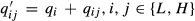
We consider a supply chain composed of a single supplier (he) and a single buyer (she). At the beginning of the season, both the supplier and the buyer have priors on the buyer's demand distribution but do not know the realization. For simplicity, we will restrict our analysis to the case where the buyer is expected to have either high (H) or low (L) demand, with priors


Below, we provide further details of the buyer's demand forecast evolution, the buyer's revenue, and the supplier's choices of contract types to offer to the buyer.
Demand Forecast Evolution
In period 1, the buyer observes a first demand signal


Table 1 summarizes the notation used in this paper.
Notation
Buyer's Revenue
We define 
These four properties are satisfied by many revenue functions commonly used in the contracting literature. Properties 1 to 3 state that the revenue increases in demand and in available supply. Property 4 guarantees the unimodality of the supplier's profit in contract quantities. We will discuss two of the most standard revenue models that satisfy these properties.


Exogenous price with salvage value
If the market is highly competitive and the buyer has limited pricing power, the retail price r is exogenous to the system. Let s, 0 ≤ s < r, be the salvage value that the buyer can obtain for each unsold unit. Then, the buyer's expected revenue is given by 

Endogenous Price
If the buyer has pricing power, then we need to define a demand response function as a function of retail price. Suppose the demand curve of type k ∈ {L, H} is linear in retail price r, and is given by 


Types of Contracts
We assume that the supplier is the leader of the game and powerful enough to offer the buyer a menu of take‐it‐or‐leave‐it contracts. If a traditional one‐time contract is to be offered, the supplier has the options to offer an early static contract or a late static contract. In the early static contract, the supplier announces the contract menu and the buyer has to choose one of the contracts on the menu after receiving her first forecast in period 1, but before receiving a more accurate second forecast in period 2. In the late static contract, the buyer obtains a forecast in period 1 and a more accurate forecast in period 2, and then selects a contract from the menu offered in period 2. In addition to the early static and late static contracts, we also consider another possibility where the supplier can offer a menu of contracts in both periods (dynamic contract). The first menu is offered in period 1, and the buyer is asked to choose a contract from the menu after obtaining the first forecast. The second menu, contingent on the first contract, is offered in period 2 and is chosen by the buyer after she has obtained the second forecast. Initially, we assume that the buyer will always obtain a more accurate forecast in period 2 regardless of the contract type offered by the supplier. We will relax this assumption later in section 5. 3
The supplier has to produce at least the quantity contracted with the buyer. He can produce in period 1 and/or period 2 but the deliveries occur at the end of period 2. The production cost in period t ∈ {1, 2} is 

Below, we discuss each type of contracts in more detail
Dynamic Contract: The supplier offers the following menu of contracts in period 1: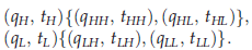
If the buyer chooses 


The supplier decides how much to produce upfront in period 1 after the buyer makes the initial selection from the period 1 menu of contracts. We define 
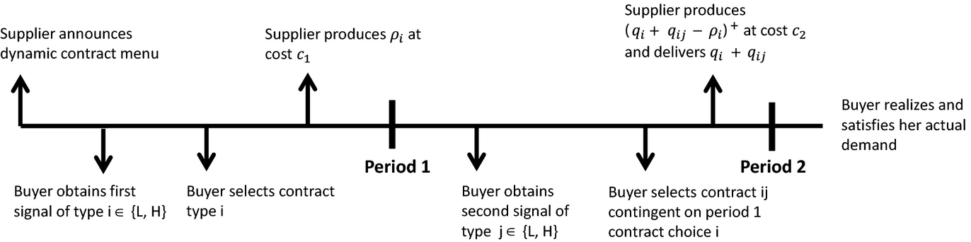
Sequence of Events: Dynamic Contract
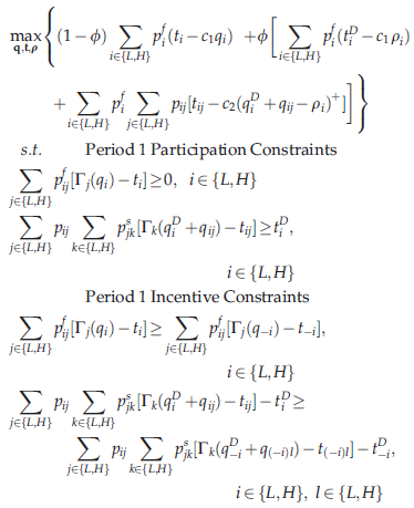
The supplier's optimization problem under the dynamic contract is given by: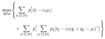

The first term in the objective function includes the initial payment and period 1 production cost 
Static Contracts
The early static and late static contracts are special cases of the dynamic contract. More precisely, under an early static contract, the supplier announces a menu of contracts 


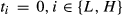
Sequence of Events: Early Static Contract
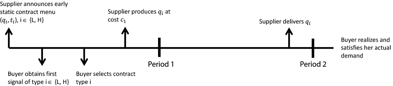
Sequence of Events: Late Static Contract
Preliminary Results
Propositions 1 through 3 characterize the structure of an optimal dynamic contract. (The proofs are provided in Appendix A.3.) We will use these properties in the next section when we discuss which contract structure (dynamic, early static, or late static) is most beneficial for the buyer or the supplier under what conditions.
Given the flexibility of the structure of the dynamic contract in our model, there are multiple dynamic contracts that result in the same expected profit for the buyer and the supplier. Proposition 1 shows that in one form of the optimal dynamic contracts, all contract quantities are deferred to the second‐period contracts (


For an optimal dynamic contract with contract quantities Similarly, we can show that the supplier can transfer the payments of the period 2 low‐type contracts to period 1 (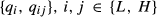

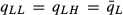
For an optimal dynamic contract with transfer payments By Propositions 1 and 2, we can construct an equivalent dynamic contract starting from any other optimal dynamic contract in the following form: 


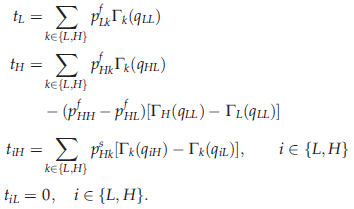
The optimal dynamic contract is not unique. All optimal contracts result in the same total order quantity, total transfer payment, and expected profit for each type of the buyer, as well as the same expected profit for the supplier. An optimal contract can be characterized as follows. If the buyer selects type i ∈ {L, H} contract in period 1, then the supplier's optimal production in period 1 is The optimal transfer payments are obtained from the binding constraints. The transfer amounts The optimal contract quantities If


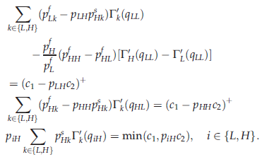


If 

Part 1 of Proposition 3 states that after the supplier learns the buyer's first signal through her contract selection in period 1, it is optimal for the supplier to produce the maximum contract quantity that the buyer may order (

An optimal dynamic contract can always be fully characterized as long as the buyer's revenue function Γ(q) is known and satisfies the properties in Assumption 1. We also note that the task of solving for the optimal transfer payments and contract quantities for a dynamic contract has essentially the same difficulty level as designing a conventional static contract. The major difference between offering a static and a dynamic contract is that a static contract distinguishes only between the two types of the buyer (H and L in period 1 or period 2); while, a dynamic contract screens for four different types of the buyer (HH, HL, LH, LL), based on all the possible combinations of the first and second signals observed by the buyer.
The fact that the optimal contract structure is not unique and that there are multiple versions of an optimal dynamic contract enables us to model many variations of contingent contracts observed in practice. For example, the dynamic contract discussed in this study can capture the contingent contracts used by a major Tier 1 auto supplier who sells to OEMs and aftermarket parts retailers. This auto supplier offers a contingent contract where the retailers are initially given a menu of quantities and prices that they can choose from. At a later date, the retailers are allowed to increase or decrease their orders. If the retailers order more, there is a per‐unit charge that is different from the per‐unit charge for the initial order. If the retailers decrease their orders, they receive money back but at a lower rate than what they have paid for the initial orders. Thus, effectively there is a penalty for the return. In the contracts that we observed, the prices for the additional orders and the penalties for the returns were clearly specified and made dependent on the magnitudes of the orders/returns. The contracts offered lower per‐unit prices for larger orders and imposed higher per‐unit penalties for larger returns. Hence, in the event that the retailers wanted to increase their orders later, they benefited from lower per‐unit prices if they had already ordered larger quantities previously.
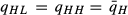
To see how this can be modeled in our framework, consider the buyer's revenue function Γ(q) = rEmin(D, q) and the following two examples:
Problem parameters: 
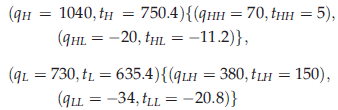
Problem parameters: 
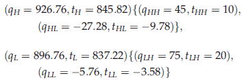
The contracts in both examples are constructed such that in the first period, the buyer commits to a quantity based on her first demand signal; in the second period, the buyer can adjust her quantity slightly up or down based on her second (more accurate) demand signal. That is, in the second period, the buyer who observes a high signal can purchase an additional quantity; while, the buyer who observes a low signal can decrease part of the quantity she has committed to in the first period for a refund. In both examples, the high‐type buyer pays a lower per‐unit price for an additional order in the second period than the low‐type buyer does (

Contract Preferences and Effect of Forecast Accuracy
We now address the question of which contracts are most profitable for the supplier or the buyer under which conditions. First, we consider the case where the buyer will always obtain a more accurate forecast in period 2. As noted earlier, early static and late static contracts are special cases of dynamic contracts. Hence, it is straightforward to see that from the supplier's point of view, dynamic contract weakly dominates early static and late static contracts. The advantage of a dynamic contract over an early static contract comes from the supplier's ability to screen not only the initial demand estimate but also the improved demand information, under the dynamic contract. This allows the supplier to potentially sell more to the buyer who observes the high‐type signal in the second period. In comparison to a late static contract, the superiority of a dynamic contract comes from its structure that enables the supplier to screen the initial demand forecast. By learning about the buyer's type upfront in period 1, the supplier can make a better production decision, resulting in cheaper production costs under the dynamic contract.
Since the supplier always prefers to use the dynamic contract (compared to early static and late static contracts), it follows directly that the supplier would always want the buyer to obtain a second (more accurate) signal. An interesting question though is whether the supplier would always benefit from increased accuracy of this second signal. Indeed, Theorem 1 shows that the better the accuracy of the signal that the buyer receives in period 2, the higher profits the supplier can realize so long as he uses the dynamic contract.
The supplier's profit under an optimal dynamic contract monotonically increases with the buyer's second‐period forecast accuracy, 
The result in Theorem 1 complements the analysis of Taylor (2006). In that paper, Taylor (using a model similar to ours but with a single‐period analysis) analyzes a situation where the buyer receives only one signal and shows that increasing the accuracy of that signal does not necessarily increase the profits of the supplier. In our setting, if the supplier used a late static contract, increasing the accuracy of 

Preferences of the High‐Type Buyer, Supplier, and Supply Chain under Exogenous Price Model:

Preferences of the High‐Type Buyer, Supplier, and Supply Chain under Endogenous Price Model:
It is also worth pointing out that the dynamic contract can be more profitable to the supplier than the early static contract even when the buyer contracting under the early static contract has an initial forecast that is more accurate than the improved forecast of the buyer contracting under the dynamic contract. That is, even when the demand information the supplier obtains from a dynamic contract is inferior to that obtained from an early static contract, the supplier's profit can still be higher under the dynamic contract. Proposition 4 provides sufficient conditions for this scenario.
Suppose that buyer A has period 1 forecast accuracy 


While the supplier can always benefit from more accurate forecasts with a dynamic contract, the contract requires that the buyer obtain a second more accurate forecast. This actually raises two interesting questions: (1) Do better forecasts also always benefit the buyer assuming the buyer has the capability to obtain them?, and (2) What would happen if the supplier is uncertain about the buyer's capability to obtain more accurate forecasts in the first place? To address these questions, we first develop an understanding of which contract is most profitable for each type of the buyer.
Proposition 5 presents the contract preferences of the low‐type buyer (who observes a low demand signal in period 1).
The low‐type buyer always prefers late static contract to early static and dynamic contract. She is indifferent between early static and dynamic contracts.
Under early static and dynamic contract, the low‐type buyer commits to the low‐type contract in period 1, before she obtains a more accurate demand forecast. Hence, she is screened as the lowest type, and is awarded zero expected profit since the low‐type participation constraints in period 1 under both early static and dynamic contracts are binding at optimality. The supplier sets the quantity and transfer payment such that the low‐type buyer makes a positive profit only if her actual demand turns out to be high‐type; she loses money ex‐post otherwise. If a late static contract is offered, however, the low‐type buyer has a chance to observe an improved demand signal in period 2, before she commits to a contract. With a positive probability, her second signal can be high‐type and she can receive a positive expected profit from the high‐type contract. If her second signal is low‐type, she receives a zero expected profit. Thus, her ex‐ante expected profit is positive under a late static contract. Since the low‐type buyer prefers to contract late and is indifferent between early static and dynamic contracts, she would always want to update her forecasts even when the supplier offers her a dynamic contract.
The situation for the high‐type buyer is different. In a screening contract, the profit to the high‐type buyer comes from the information rent that the supplier has to offer in order to prevent the high‐type buyer from deviating to lower type contracts. Hence, the high‐type buyer always makes positive profits under all three types of contracts. However, it is not immediate which type of contract the high‐type buyer would prefer. Proposition 6 shows that the high‐type buyer always prefers to contract early rather than dynamically. Furthermore, under the dynamic contract, the high‐type buyer's expected profit decreases as her second‐period information accuracy improves. This is because under early static contract, the buyer only reveals her less accurate demand information, leaving sufficient amount of uncertainty which results in higher rents. On the other hand, the buyer reveals both her initial and improved demand information under dynamic contract, leaving little rents to her. The additional demand information revealed in the second period always benefits the supplier rather than the buyer because it decreases the uncertainty about the buyer's type.
The high‐type buyer's profit under the early static contract is at least as high as her profit under the dynamic contract. The high‐type buyer's profit under the dynamic contract monotonically decreases with the second‐period forecast accuracy. Since the early static contract is more profitable to the high‐type buyer than the dynamic contract, if the buyer expects that the supplier would offer her a dynamic contract, she may try to opt out from obtaining a second forecast, in order to be offered an early static contract instead, by claiming that she is incapable of conducting a more accurate forecast. Of course, a powerful supplier who is certain that the buyer is capable can simply offer a take‐it‐or‐leave‐it dynamic contract to the buyer. But what if the buyer could really dictate the decision whether to update her forecasts, would the supplier still be able to benefit from more accurate forecasts? In this case, if both the supplier's and the buyer's profits are higher with the late static than with the early static contract, the supplier can benefit from offering the late static contract upfront (in a sense, take the dynamic contract off the table). Then, both parties can still benefit from more accurate demand information. An example of such a situation where the late static contract is more preferable to both parties than the early static contract is shown in Figure 4, when the period 2 accuracy,


This section has shown that while the supplier always benefits most from, and therefore, favors the dynamic contract, the buyer may actually prefer the early static contract and may try to claim that she is incapable of obtaining a more accurate demand forecast in the second period. A powerful supplier who is certain that the buyer is capable can simply impose a take‐it‐or‐leave‐it dynamic contract. However, if the supplier is uncertain about the forecasting capability of the buyer, the supplier may want to consider offering a contract that screens both the capability and the demand type of the buyer. We study such contracts in the next section.
Screening the Forecasting Capability
In many situations, the supplier may not be certain whether the buyer can update forecasts closer to the selling season or not. This is likely to be the case for a supplier and a buyer who enter into a contract with each other for the first time. Even for a supplier and a buyer who have contracted before for other items, if the buyer is purchasing a new item or introducing a new product to the market, the supplier may not have enough information to deduce the buyer's forecasting capability. For example, consider the toy industry. Every year, Mattel introduces new toys. The retailers often order some toys initially after Mattel displays the toys in a trade show, and order more later after they update their forecasts. A toy release is often linked to an advertising campaign, or a movie release. These campaigns generally start in large markets. A big retailer like Walmart who has stores all over the United States can monitor early sales in test markets and update its forecasts quickly for all of its stores. On the other hand, Mattel is much less certain about the forecast capability of a small retailer in a remote rural area. Even with repeated interactions, products in this industry change very frequently and past success in forecasting demand for one type of products may not translate into success in forecasting demand for another type of products.
The model in this section also applies to a situation where the forecast updates are costly, but the supplier is uncertain about the buyer's forecasting costs, as modeled by Lariviere (2002). That is, the buyer may incur a small update cost or a large update cost. If the buyer's update cost is small, then it is worthwhile for the supplier to induce the buyer to obtain improved forecasts using a dynamic contract. On the other hand, if the buyer's update cost is large, then the supplier prefers to contract with the buyer under an early static contract. 5 In this case, the large update cost will never be incurred (since the buyer is offered an early static contract). Then, the buyer with a small update cost is equivalent to the capable buyer (forecaster), and the buyer with a large update cost is equivalent to the incapable buyer (nonforecaster) in this model.
When the supplier is uncertain as to how accurate of a demand forecast the buyer can obtain, we propose that the supplier can improve the screening nature of his contracts by screening the buyer not only on demand level, but also on forecasting capability. Suppose that the supplier has a prior on the capability of the buyer to obtain improved forecasts. The supplier can design a capability‐and‐type screening menu of contracts such that the capable buyer prefers dynamic contract, and the incapable buyer prefers early static contract.
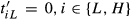
The capability to obtain a better demand forecast is private information to the buyer. However, we assume the supplier estimates that with probability ϕ, the buyer is capable of obtaining a more accurate demand forecast, and with probability 1 − ϕ, she is not capable. The capable buyer is simply the buyer described in previous sections, who receives a more accurate forecast in period 2. On the other hand, the incapable buyer observes a signal whether she is low‐type or high‐type in period 1, but is incapable of making that forecast more accurate in period 2. Since the incapable buyer does not receive a more accurate signal, if she purchases a dynamic contract, she uses a strategy such that with probability 
The supplier offers a menu of contracts that screens both the type and forecasting capability of the buyer. He offers a menu of the early static contract, 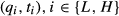


In this setting, we have the following results regarding the supplier's and the buyer's optimal strategies and profit.
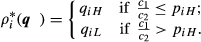
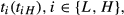
Under an optimal two‐dimensional screening contract: The optimal strategy for the incapable type i buyer if she were to contract dynamically is to choose the iL contract in period 2 with probability 1, that is, Both capable and incapable buyers of the same type receive the same expected profit, where the profit is zero for the low‐type buyer and is positive for the high‐type buyer. The supplier's profit monotonically increases with the capability probability ϕ and the period 2 forecast accuracy The high‐type buyer's profit is monotonically decreasing in the capability probability ϕ and is independent of period 2 forecast accuracy Parts 1 and 2 of the theorem are driven by the binding constraints in an optimal two‐dimensional screening contract. More precisely, when the buyer is incapable of obtaining a more accurate demand signal to help her decide which contract to choose in the second period, she minimizes her risk of losing money from ordering too much by always relying on the low‐type contract. This is because an optimal screening contract is designed such that the high‐type buyer's expected profit from deviating to the low‐type contract is the same as the expected profit from choosing the high‐type contract; however, the low‐type buyer could lose money from deviating to the high‐type contract. The forecasting capability incentive constraints are also binding at optimality, resulting in the same expected profit to the capable and incapable buyer of the same type. Like under other screening contracts, the low‐type expected profit is zero, while the high‐type expected profit is positive due to the information rents.


Parts 3 and 4 of the theorem describe the effects of the capability probability as well as the second forecast accuracy on the supplier's and the high‐type buyer's expected profit. In section 4, it has been shown that the supplier always prefers dynamic contract; while, the high‐type buyer always prefers early static contract to dynamic contract. Hence, as the capability probability increases, the high‐type buyer's expected profit is reduced but the supplier's profit is increased. Figure 6a and b display the expected profits of the high‐type buyer and supplier for different values of capability probability. (Note also that an increase in the market uncertainty δ benefits the buyer and hurts the supplier as expected.) If instead the capability probability is fixed, but the capable buyer's second forecast accuracy is improved, we show that the supplier can continue to take advantage of the buyer's better demand information. This result is consistent with Theorem 1, where we show the supplier is better off contracting with a more accurate buyer using a dynamic contract. What is less expected here is that a change in the capable buyer's improved forecast accuracy has no effect on the buyer's expected profit. This is because the second‐period forecast accuracy only influences the performance of the capable buyer, but not the incapable buyer. Since the supplier's belief about the buyer's forecasting capability is not affected and since it is optimal to offer both capable and incapable buyer the same profit, the supplier gives the same optimal level of rent to the buyer, and keeps the remaining increase in supply chain profit due to better forecast accuracy to himself.

High‐Type Buyer's and Supplier's Profits under Two‐Dimensional Screening Contracts:
We have shown that even in the presence of the uncertainty about the buyer's forecast capability, the supplier can still always benefit from more accurate demand information if he uses a dual‐screening contract. It is also interesting to explore whether other mechanisms could provide similar benefits. In particular, we would like to compare the performance of the dual‐screening contract to that of the buy back and quantity flexibility contracts studied in Lariviere (2002). For our setting with two types of demand, we consider the buy back and quantity flexibility contracts such that the supplier offers four types of contracts in period 1, meant for the low‐type forecaster (LF), high‐type forecaster (HF), low‐type nonforecaster (LN), and high‐type nonforecaster (HN). The buy back contract meant for the type‐ij buyer, i ∈ {L, H}, j ∈ {F, N}, is characterized by two parameters: a wholesale price 


We numerically compare the three contract types: dual‐screening, buy back, and quantity flexibility, with the first‐best contract (no information asymmetry) as a benchmark, assuming an exogenous price model with a uniformly distributed ε. 6 Table 2 summarizes the comparison results for different values of capability probability ϕ and demand uncertainty δ.
Comparison of the Supplier's Profit under Dual‐Screening, buy Back, and Quantity Flexibility Contracts: 
We find that the supplier's profits under buy back and quantity flexibility contracts behave similarly to the supplier's profits under dual‐screening contracts with respect to ϕ and δ. That is, under the two restricted return contracts, the supplier's profits also decrease with δ but increase with ϕ, similar to what is shown in Figure 6bfor the dual‐screening contract. We find, however, that the supplier's profits with restricted return contracts are smaller than the profits with dual‐screening contracts. As shown in Table 2, the dual‐screening contract is increasingly more profitable than the two restricted return contracts and is also performing closer to the first‐best contract as the buyer is more likely to be capable of improving forecast accuracy. This implies that the more elaborate structure of the dual‐screening contract is more effective in extracting benefits from the capable buyer's more accurate information than the simpler structure of a restricted return contract. Hence, if the supplier believes the buyer is highly likely to be capable of improving her forecasts, then it is worth offering a more sophisticated contract like a dual‐screening contract to maximize his expected earnings. If the buyer is not likely to be capable, however, the supplier may consider using a simpler restricted return contract which would still gives him most of the benefits.
We also note that between the two restricted return contracts, the buy back contract performs better than the quantity flexibility contract in most cases, which is the same observation as in Lariviere (2002). However, while Lariviere (2002) finds that quantity flexibility contracts can be better than buy back contracts when forecasting cost is very expensive, we find that quantity flexibility contracts can be better when δ and ϕ are sufficiently large. This is because when δ is large, more accurate forecasts do not offer much value as the demand uncertainty is still high. But when ϕ is large, the supplier has to pay high rent to the capable buyer. In this case, amount of returns are expected to be large after the actual demand is resolved. Hence, being able to limit the return amount with a quantity flexibility contract is more effective than being able to limit the refund rate with a buy back contract. Finally, we observe that if the demand uncertainty is not very large and the probability that the buyer is capable is significant, then the performance of the dual‐screening contract is very close to that of the first‐best contract.
The results in this section show that there exist mechanisms which allow the supplier to always benefit from more accurate demand information even when he is not certain about the buyer's forecasting capability. An implication here is that more accurate information is always potentially beneficial to the supplier as long as he designs contracts wisely.
Conclusion
In this study, we consider a stylized model of a multiperiod procurement game between a powerful supplier and a buyer under demand information asymmetry. We investigate whether and when the parties benefit from the buyer's more accurate demand forecasts under different contract structures. A key finding of our paper is that a supplier who knows that a buyer is capable and is going to obtain more accurate forecasts can always benefit from the buyer's improved demand information by offering a dynamic contract, which screens both the buyer's initial and improved forecasts. This result complements what has been found in the existing supply chain contract literature which mostly considers simple static contracts and reports that the supplier's profit can be hurt by improved demand forecasts from the buyer. An interesting situation is when the supplier may be uncertain about the buyer's capability (or forecasting cost) to obtain more accurate forecasts. In this case, the buyer may argue that her costs to obtain more accurate forecasts are too high, especially when better forecasts are likely to hurt her profits. But in response, we show that the supplier can offer a more sophisticated contract to screen the buyer both on her forecast updating capability (equivalently forecasting costs) and demand type.
An important conclusion of our study is that suppliers can always benefit from the buyers’ demand forecasts that become more accurate over time. However, to achieve this benefit, the supplier may sometimes be required to design more sophisticated contracts, for example, with contingent clauses. As noted earlier in this study, contingent contracts have recently been observed in practice; for example, a major Tier 1 auto supplier uses a contingent contract when selling to aftermarket parts retailers. We also show that if the supplier is uncertain about the buyer's forecasting capability, then even the standard contingent contracts may not be enough. In this case, the supplier may have to develop dual‐screening contracts, which have been much less common in practice. Our finding indicates that there may be a certain point in the supply chain contract's complexity level where the benefit obtained by the contract is outweighed by its complexity. Further research is needed on simpler mechanisms that achieve most if not all of the more sophisticated mechanisms developed here.
Footnotes
Characterization of Optimal Contracts
Contract Preferences
Acknowledgments
The authors are grateful to constructive comments from the editor and the referees which helped improve the paper significantly throughout the review process.
1
Notice that
2
3
Note that in all our models, the buyer is never asked to choose a contract from the menu before obtaining at least one forecast of her demand. Of course, one could plausibly also consider the scenario where the supplier forces the buyer to choose a contract at time zero before the buyer has even obtained a first signal. Comparing early static and dynamic contract offered at time 0 and late static contract offered after the buyer has obtained a more accurate forecast will not change our conclusions that dynamic contract is most profitable for the supplier, and that under a dynamic contract, the supplier always benefits from the buyer's updating of her forecasts. In actual supply chains, some information asymmetry between supplier and buyer always exists, and we have not come across many buyers who sign contracts before they have any idea what their demand is going to be. Thus, in our models we let the buyer choose a contract only after she has obtained at least one demand signal.
4
We assume that the inventory holding cost between period 1 and 2 is negligible without loss of generality.
5
When forecast updates are costly, the update cost is ultimately transferred to the supplier through the contract design (in a form of reduced transfer payments, required to satisfy the participation constraints of the buyer). Hence, it is profitable for the supplier to contract dynamically only when the update cost is no greater than the extra profit the supplier can gain from dynamic contract over early static contract.
6
Forecast update costs are normalized to 0.