Optimal Choice for Appointment Scheduling Window under Patient No‐Show Behavior

Introduction

Appointment scheduling systems are widely used by healthcare providers to regulate their service capacity and patient demand. Providing patients with pre‐scheduled appointments reduces the variability in demand, and allows providers to better plan their daily operations. However, not every patient will show up for their scheduled services, creating the commonly known patient “no‐show” problem. Many health service providers report high no‐show rates which can range from 23% to 34% (Dreiher et al. 2008, Geraghty et al. 2007). No‐shows leave appointment slots wasted, and can result in significant financial loss (Atun et al. 2005, Moore et al. 2001). No‐shows also break continuity of care, and may lead to poor patient health outcomes (Nguyen et al. 2011, Schectman et al. 2008).

To mitigate the impact of no‐shows, healthcare providers can try directly improving patient attendance via sending reminders, providing transportation assistance or charging no‐show fees, but these interventions cannot completely eliminate no‐shows (Guy et al. 2012, Macharia et al. 1992). Some clinics still faced 20% or higher patient no‐show rates even after implementing appointment reminder systems (Geraghty et al. 2007, Hashim et al. 2001).

Facing high patient no‐show rates, providers can also consider adjusting their operations. One commonly adopted strategy is to overbook, that is, to schedule multiple patients in one appointment slot to hedge against the risk that some of them do not show up. The overbooking strategy has been studied extensively in the Operations Management (OM) literature; see, for example, LaGanga and Lawrence (2007), Muthuraman and Lawley (2008) and Zeng et al. (2010). The second operational lever often used by practitioners is to control the panel size, that is, the number of patients a practitioner considers as her “own” patients (Green and Savin 2008, Liu and Ziya 2014). This operational lever is motivated by observing that patients tend to have higher no‐show probabilities when their appointment delays are longer (Dreiher et al. 2008, Gallucci et al. 2005, Liu et al. 2010). The appointment delay is the scheduling interval, that is, the time between the day when a patient requests for an appointment and the actual appointment date given to her. By limiting the panel size, a provider can ensure that her patients will not wait too long for appointments and thus will be more likely to show up.

Though panel size selection and overbooking are widely used operational levers to cope with patient no‐shows, they may not be implementable in a large number of practices. For instance, 1128 community health centers in the U.S. are Federally Qualified Health Centers (FQHCs) as of 2011, and they receive government grants under the Public Health Service Act (Shin et al. 2013, U.S. Department of Health and Human Services 2014). In return for these grants, FQHCs have to serve all patients regardless of their ability to pay (Rural Assistance Center 2013). Consequently, providers in these centers cannot “dismiss” patients from or “reject” new patients to join their panels like their counterparts in private practices. In addition, providers in community health centers are often salaried, meaning that their incomes do not depend on the volume of patients they see and there is little financial incentive for them to work overtime. Overbooking, which often causes overtime work, is therefore unwelcome from these providers’ perspectives and can be difficult, if not impossible, to implement.

Without the options of overbooking or controlling panel size, one important and practical operational lever left to deal with appointment delay‐dependent patient no‐shows is to limit the appointment scheduling window. That is, patients are not allowed to make appointments beyond a certain day from the day when they make appointments. When there are no appointments slots available within the appointment window, providers usually have two ways to handle additional patient requests if any. One option is to simply advise patients to seek care elsewhere, for example, urgent care centers nearby. This option avoids overtime for providers. The other option is to accommodate these patients via working beyond the regular appointment hours. Although this option cannot circumvent overtime, it is still considered more acceptable by physicians than directly asking them to overbook. The reasons are mostly psychological. First, shortening the appointment scheduling window can be naturally phrased as a means to reduce delays and improve access to care, which are aligned well with healthcare providers’ professional pursuit. Second, overtime that may result from shortening the appointment window is not directly“built” into the system, and thus is less “repelling.”

In our discussion with health care professionals, we learned that controlling the appointment window is a commonly‐used operational lever in community health centers. Some centers have the same rule for all patients, while others may set different rules depending on patients’ no‐show behaviors. For example, one community health center in New York City faces 30–40% patient no‐show rates; it prohibits “frequent no‐show offenders” (defined as patients missing appointments more than five times in the past year) from making appointments one day ahead, but it is committed to serving these patients on an as‐needed basis (D. Rosenthal 2011, Columbia University, pers. comm.). Similarly, Wingra Family Medical Center, a large urban residency teaching clinic of the University of Wisconsin Family Medicine Residence Program, only permits patients who had demonstrated high appointment adherence in the past to schedule appointments in advance (DuMontier et al. 2013). However, there seems to be no consensus on when and how to use such an operational lever, and practices largely rely on trial‐and‐error approaches, often resulting in inefficiency and suboptimal management. It is the operational challenge faced by these practices that motivates our research.

Limiting the appointment scheduling window reduces appointment delays and thus no‐shows, leading to more efficient use of appointment slots. However, an overly restrictive scheduling window may leave too many patients unable to schedule their appointments. These patients may either seek care elsewhere or arrive at the clinic requiring service during overtime, resulting in some form of penalty to the provider either as loss of revenues, loss of goodwill from patients or unplanned overtime work for staff. Intuition seems to suggest that using a shorter appointment window for patients with higher no‐show rates would increase efficiency, but is this intuition correct? More generally, how does the choice of appointment scheduling window affect a provider's operational efficiency? Furthermore, how much efficiency gain can be achieved by adopting an optimal appointment window, when practices may (or may not) have the options to select panel size and overbooking level? This study seeks to answer these important questions unaddressed in the previous OM literature.

In this study, we develop stylized models as a simplified version of reality, which allow us to draw high‐level managerial insights. This serves as a first step to tackle the challenges faced by those providers in using the appointment scheduling window as an operational lever to deal with patient no‐shows. Using a single server queue model motivated by the work of Green and Savin (2008) and Liu and Ziya (2014), we are able to fully characterize the optimal appointment window and show how this optimal appointment window should be adjusted in response to changes in other model parameters. These results inform the conditions under which a longer appointment window may benefit practices more (or less). In addition, we carry out extensive numerical studies, which are based on carefully chosen model parameters, to strengthen our analytical findings. In particular, we investigate the efficiency gain of adopting an optimal scheduling window when a practice has (or does not have) the options of selecting panel size or overbooking levels. Finally, we extend our analytical model to consider a patient population with heterogeneous no‐show behaviors.

Our work is particularly related to appointment scheduling literature that develops operational strategies to deal with patient no‐shows. Depending on the planning horizon, this literature can be grouped into the work on intra‐day scheduling and the work on inter‐day scheduling; see Cayirli and Veral (2003) and Gupta and Denton (2008) for an in‐depth review.

Intra‐day scheduling concerns the best timing and sequence of appointments within a given day in order to optimize the trade‐off between patient in‐clinic waiting and provider utilization (taking patient no‐shows into account); see, for example, Hassin and Mendel (2008) and Robinson and Chen (2010). Inter‐day scheduling literature considers patient scheduling in a multi‐day planning horizon. The decision maker determines how to allocate appointment requests arising on the current day into future days; see, for example, Patrick et al. (2008) and Liu et al. (2010). Our work departs from the previous literature in that we consider a fundamentally different decision problem and focus on a more strategic level of decision making. We determine the size of the appointment window, that is, we consider how long in advance an appointment should be allowed to be scheduled, when patients exhibit delay‐dependent no‐shows.

The two articles most relevant to ours are Green and Savin (2008) and Liu and Ziya (2014). Similar to ours, both articles use a single server queue to model an appointment system where patient no‐show probabilities increase with appointment delays. However, there are a number of crucial differences distinguishing our work and theirs. The objective of Green and Savin (2008) is to identify a panel size sustainable for a practice to use Open Access, but our motivation is to find a proper appointment window that maximizes the efficiency. Accordingly, the decision variable in Green and Savin (2008) is the patient demand rate, while ours is the capacity of the appointment queue. In terms of the analysis, Green and Savin (2008) develop approximate methods to evaluate system performance; we focus on deriving structural results and obtain insights on what affect the optimal decisions and the system performance. The models in Liu and Ziya (2014) have an objective that shares a similar flavor as ours. However, they seek to jointly determine the optimal panel size and overbooking level which maximize the system efficiency. They do not impose a limit on the appointment window. In contrast, we study completely different operational strategies to deal with no‐shows by controlling the appointment window. In addition, Liu and Ziya (2014) only consider a homogeneous patient population, whereas we also study a model in which patients are heterogeneous in their no‐show behavior. These distinctions lead to different models and analyses, and bestow new managerial insights.

The rest of the article is organized as follows. Section 2 describes our model and the analytical results. Section 3 presents our numerical study. Section 4 discusses the model extension with heterogeneous patients. Section 5 provides the concluding remarks. The proofs of all the analytical results can be found in Appendix S1.

Model

We consider a single provider service system where the provider can control the appointment scheduling window. Our objective is to investigate how the size of the scheduling window affects system performance. Following the earlier work in Green and Savin (2008) and Liu and Ziya (2014), we use a single server queue as a stylized model to represent the appointment schedule of a provider. In the rest of the article, we use the words patient(s) and customer(s) interchangeably.

Suppose that the provider has an established panel of patients. Appointment requests from any patient in this panel arise according to a Poisson process, independent from those of others. Thus, the overall demand to the provider also follows a Poisson process. We assume that the overall demand rate is λ > 0. We further assume that patients have strong preferences on speedy access to care, and thus they will be (offered and) scheduled to the earliest appointment slot available. Patients may have other preferences for appointments (e.g., time of day), but our model is likely to be a reasonable approximation for reality if most patients strongly desire shorter appointment delays. Although academic literature on patient preferences for appointment scheduling is relatively scant, one study by Murray and Tantau (2000) suggests that only 25% of patients who are offered same‐day appointments opt to see a physician at a later time, supporting our assumption.

We keep a track of the appointment backlog of the provider, and refer to it as the “queue.” This queue is in fact a virtual waitlist of scheduled patients yet to be seen by the provider. We assume that patients will not cancel their appointments, and thus the new appointment requests always join the queue from the very end. This assumption usually works well for community health centers, which motivate our research. As Medicaid does not allow patients to be billed for missed appointments, these practices do not charge patients for failing to cancel scheduled appointments early enough. As a result, patients often“forget” about making cancellations.

To better interpret how our model approximates reality, imagine for now that each appointment slot is deterministic with length 1/μ day. The actual service time may have some variability, but it suffices to assume that the provider can serve each patient within one appointment slot. Or equivalently, we can imagine that the provider has exactly μ appointment slots in a day, and she will not overbook.

Consider the following sequence of events in an appointment scheduling system. During the day, patients make requests for appointments. Because the length of each appointment slot is deterministic, the provider knows exactly when the next available appointment is, and she will schedule the incoming patient to that slot. As time passes, the provider serves the patients on the schedule and makes the queue shorter. When the provider is off duty, no patients call in to join the queue and no patients are served or leave the queue either; the queue remains unchanged. Observing this, we can “drop” the non‐office hours of the provider and “coalesce” the office hours together to consider a continuous queueing process.

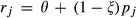
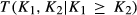
When patient appointment times come, they arrive on time if they show up, but they may not show up for their appointments. We assume that if there are j patients in the system when a new patient makes the appointment request, this new patient will be scheduled as the (j + 1)th patient in the system and show up with probability

p j ∈ [ 0 , 1 ]

p j ≥ p j + 1

p ∞ = lim j → ∞ p j

p j > p k

p 0 > 0

Each scheduled patient who shows up brings in one nominal unit of revenue. If a patient does not show up, the provider cannot serve the next patient right away because every patient is scheduled and they will not come until their scheduled time slots. This can also be thought of as that the provider is “serving” the appointment slot of this no‐show patient before moving to the next one. Without loss of generality, we assume that if a patient does not show up or there are no patients scheduled in the current slot, the provider is able to fill in the slot by completing one ancillary task. Examples of these ancillary tasks include follow‐up service coordination for a patient, checking lab results, consulting with a patient's other providers and responding to a patient's email or phone call. These tasks may be billable to some (but not all) payers and typically with a lower reimbursement rate compared to that of direct patient care service (Merrell and Berenson 2010). To capture this, we assume that a revenue of ξ ∈ [0,1) is generated for each of these tasks (we call ξ the ancillary task revenue rate). We further assume that patient arrivals preempt ancillary tasks. That is, when an actual patient arrives, physician stop doing ancillary tasks if any and turn to serving the arriving patient. This assumption is certainly reasonable when ancillary tasks are interruptible as many are, such as replying to patients’ emails. We also make this assumption to keep our models tractable.

The service provider has control over the appointment scheduling window, that is, how far into the future a new appointment can be scheduled. Since the length of each appointment slot is deterministic, this is equivalent to controlling the queue capacity, which we denote by K. If the current length of the appointment queue is less than K, the provider will schedule new patients when they arrive. However, if there are already K patients in the queue (including the one in service), the provider will not schedule the incoming patient. This action incurs a penalty cost of θ ≥ 0 per patient. This is to capture the fact that this “rejected” patient may choose to seek care elsewhere resulting in loss of revenues to the provider or she may have to be accommodated using overtime work at additional cost (more on this below). The goal of the service provider is to maximize the long‐run average net reward, that is, revenue less cost, by choosing a proper queue capacity K. Put into the original operational context, setting a queue capacity K is equivalent to choosing an appointment scheduling window to be K/μ days.

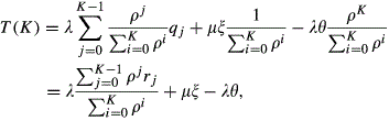
Let T(K) denote the long‐run average net reward collected by the system. Define

Π j ( K )

q j = p j + ( 1 − p j ) ξ = ξ + ( 1 − ξ ) p j .

0 ≤ q j + 1 = ξ + ( 1 − ξ ) p j + 1 ≤ ξ + ( 1 − ξ ) p j = q j ≤ 1

q j

q ∞

T ( K ) = λ ∑ j = 0 K − 1 Π j ( K ) q j + μ ξ Π 0 ( K ) − λ θ Π K ( K ) .

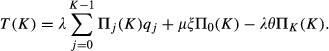
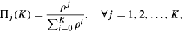
The first term on the right side of Equation 2 is the revenue obtained from patients who showed up for their scheduled appointments and ancillary tasks completed in place of no‐show patients. The second term is the revenue obtained from ancillary tasks when there are no scheduled patients in the queue. To be specific, we note that the steady‐state probability that the server has no scheduled customers waiting is

Π 0 ( K )

Π 0 ( K ) μ

μ ξ Π 0 ( K )

λ Π K ( K )

max K ∈ Z + T ( K ) ,

P1

Z + = { 1 , 2 , 3 , … }

Although we can numerically calculate

Π j ( K )

Π j ( K )

Π j ( K ) = ρ j ∑ i = 0 K ρ i , ∀ j = 1 , 2 , … , K ,

T ( K ) = λ ∑ j = 0 K − 1 ρ j ∑ i = 0 K ρ i q j + μ ξ 1 ∑ i = 0 K ρ i − λ θ ρ K ∑ i = 0 K ρ i = λ ∑ j = 0 K − 1 ρ j r j ∑ i = 0 K ρ i + μ ξ − λ θ ,

r j = θ + ( 1 − ξ ) p j

r j

Optimal Capacity for the Appointment Queue

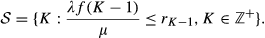
In this section, we derive the optimal capacity for the appointment queue. For ease of discussion, we let

f ( K ) = ∑ j = 0 K − 1 ρ j r j ∑ i = 0 K ρ i , K ∈ Z + ,

and define f(0) = 0. Then, the net reward function T(K) can be rewritten as

T ( K ) = λ f ( K ) + μ ξ − λ θ .

We can show the following results.

Proposition 1

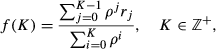
For any fixed λ,μ > 0, net reward T(K) is a quasi‐concave function of K over

K ∈ Z +

. Furthermore, the largest maximizer

K *

is given by

K * = sup { K : K ∈ S }

where

S = { K : λ f ( K − 1 ) μ ≤ r K − 1 , K ∈ Z + } .

Our intuition suggests that there exists a trade‐off between choosing a larger K vs. a smaller K. When the appointment queue capacity is larger, fewer patients are “rejected” but patient delay is longer leading to more no‐shows and diminishing efficiency. When K is smaller, patients scheduled are more likely to attend their appointments but the provider leaves a larger proportion of patients unscheduled, resulting in lower revenues and more non‐scheduling penalties. Proposition 1 confirms our intuition above and establishes that the net reward is a weakly unimodal function of the appointment queue capacity K. To give an intuitive explanation, recall from Equation 1 that the expected revenue from scheduling a patient with j appointments ahead is

p j + ( 1 − p j ) ξ

. However, if this patient is “rejected”, the revenue collected during the slot time which could have been scheduled for this patient is ξ − θ. As

r j

's used in Equation 5 and Proposition 1 can be rewritten as

r j = θ + ( 1 − ξ ) p j = [ p j + ( 1 − p j ) ξ ] − ( ξ − θ ) ,

r j

can be interpreted as the additional expected revenue of scheduling a patient with j appointments ahead upon her arrival rather than “rejecting” her. Proposition 1 suggests that

K *

depends on such revenue margins. More specifically, the daily net reward T(K) can be decomposed into two parts, the constant part being the revenue of just doing ancillary tasks and not accepting any patients (i.e., μξ − λθ), and the variable part being the “top‐up” revenue if accepting at most K patients in the system (i.e., λf(K)). Then Proposition 1 says that if

r K − 1

, the marginal revenue of accepting the Kth patient (who sees K − 1 patients ahead) into the system, is larger than the long‐run average top‐up revenue per appointment slot of allowing at most K − 1 patients in the system, then the Kth patient should be accepted.

As a direct result from Proposition 1, we obtain the following Corollary, which identifies a necessary condition for

K *

when it is finite.

Corollary 1

If

K = K * < ∞

, then

r K < r K − 1

.

Corollary 1 implies that the optimal appointment queue capacity occurs at some integer K where the value of

r K

has a strict drop from

r K − 1

. This result is quite useful in devising simple algorithms to find

K *

. In particular, to search for

K *

one only needs to check the integers at which the value of

r K

has a strict decrease. In addition, if patient no‐show probabilities depends on appointment delays (in days), that is,

p j

changes only if ⌊j/μ⌋ changes, then

K *

would be multiples of the daily service capacity μ, automatically making the optimal appointment window

K * / μ

an integer number (see more discussions in section 3).

Sensitivity Results

The last section investigates the property of the net reward function and how to find the optimal appointment queue capacity

K *

. In this section, we study how

K *

changes with respect to changes in other model parameters, such as show‐up probabilities

{ p j }

and appointment demand rate λ. These sensitivity results are useful for managers to adjust an appointment system if the practice environment changes.

We first investigate how the adoption of a new intervention (e.g., use of a reminder system) that is expected to change no‐show probabilities affects the optimal appointment queue capacity. We use

{ p j } j = 0 ∞

to denote the current show‐up probabilities and

{ p ^ j } j = 0 ∞

to denote the show‐up probabilities post intervention. We also let

K ^ *

denote the optimal queue capacity for the new system. We are interested in the following question: if show‐up rates increase under the intervention, that is,

p ^ j ≥ p j

for j = 0, 1, 2, …, does it mean that

K ^ *

should be larger than

K *

?

Intuition might suggest that if patients have higher show‐up probabilities, then the system can use a longer appointment queue to optimize the system performance because patients are more “reliable.” The argument is that, since patients are more likely to attend the appointment given the same appointment delay, the clinic can have a longer appointment queue to keep scheduled patients. It is true that keeping a longer appointment queue in a system with higher patient show‐up probabilities might still achieve an equal or even better net reward compared to a system with lower patient show‐up probabilities, because scheduled patients are more likely to come and the non‐scheduling penalty is smaller with a longer appointment window. However, the objective here is not to maintain or simply beat the same reward level as a system with low patient show‐up probabilities, but rather to optimize the reward rate under high patient show‐up rates. Thus, the intuition above is flawed, as demonstrated by the following example.

Example 1

Suppose that the average daily capacity of the clinic is 20, that is, μ = 20 and appointment arrival rate λ = 17. Let

p j = ( 0.9 ) j + 1

for

j ∈ Z

,

p ^ 0 = 1

,

p ^ 1 = 0.9

, and

p ^ j = ( 0.9 ) j + 1

for j ∈ {2,3,…}. Thus,

p ^ j ≥ p j

for all

j ∈ Z

. For simplicity, we assume that ξ = θ = 0. Then, one can show that

K * = 5

while

K ^ * = 4

, meaning that the optimal appointment queue capacity is smaller even when patients are more likely to show up.

Example 1 implies that following one's intuition to adjust appointment queue capacity can be counterproductive. Then, one question arises naturally: what conditions, if any, would ensure that

K ^ * ≥ K *

? A closer examination of Proposition 1 reveals that the key determinant for

K *

is when

r K − 1

, the additional expected revenue of scheduling a patient rather than “rejecting” her, stops being larger than f(K−1) (see Equation 6). Note also that f(K − 1) can be regarded as a “weighted” average of

r j

's for j = 0, 1, …, K−2. Thus, one may contend that

K *

should depend more on how

r j

's (or equivalently

p j

's) change in j, rather than the magnitudes of

p j

's. The ensuing discussion will quantify this contention. Consider the following condition. We define

p − 1 = p ^ − 1 = 0

for notational convenience.

Condition 1

p ^ j − 1 − p ^ j ≤ p j − 1 − p j

for j = 0,1,2,….

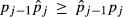
Condition 1 requires that after the intervention, the decrease in show‐up probability with additional appointment delays is smaller compared to that under the original system. That is, patients are less “sensitive” to additional delays in the new system. Condition 1 also implies that

p ^ j ≥ p j

, j = 0,1,2,…. With Condition 1, we can show the following results.

Proposition 2

If condition 1 holds and other model parameters are fixed, then

K ^ * ≥ K *

.

It is interesting to note that when θ = 0, that is, when the non‐scheduling penalty is zero, the following condition, slightly weaker than condition 1, guarantees Proposition 2 to hold.

Condition 2

p j − 1 p ^ j ≥ p ^ j − 1 p j

for j = 0,1,2,….

Condition 2 requires that

p ^ j p ^ j − 1 ≥ p j p j − 1

when

p ^ j − 1 , p j − 1 > 0

. This can be thought of as another form to rank patient sensitivity to delays. Patients with

p ^ j

's are less sensitive to those with

p j

's because the percentage drop in show‐up probabilities for

p ^ j

's with additional appointment delays is smaller than that of

p j

's. These conditions will be useful in the discussion of our numerical results in section 3.

We now study how the provider should adjust the capacity of appointment queue in response to changes in other model parameters, including the demand level λ, service rate μ, non‐scheduling penalty rate θ and ancillary task revenue rate ξ. We are able to establish the following monotonic relationships.

Proposition 3

Other model parameters being fixed, the optimal capacity for the appointment queue,

K *

, is

decreasing in the demand rate λ;

increasing in the service rate μ;

increasing in the non‐scheduling penalty rate θ;

increasing in the ancillary task revenue rate ξ.

In this study, we use the terms “increasing” and “decreasing” to mean “non‐decreasing” and “non‐increasing,” respectively. Proposition 3 states that as the appointment demand increases, the service provider should be stricter and allow fewer outstanding appointments. This might sound counterintuitive at first. In response to a surge in demand, one might be tempted to allow more appointments to benefit from the increase. However, in fact, the increase in demand is all the more reason to limit the size of the appointment queue. Higher demand means less need to accumulate customers in the queue since the service provider has less trouble filling the empty appointment slots. For a fixed appointment queue capacity, higher demand means longer customer wait time and thus higher no‐show rates. Reducing appointment queue capacity in this case leads to shorter appointment delays and thus reduces no‐shows. The revenue gains outweigh the cost of having more patients unscheduled due to reducing the appointment window. In short, this result suggests that for efficiency‐maximizing service providers who experience high demand, there may be fewer incentives to offer appointments far into the future.

The other three monotonic relationships seem to follow our intuition well. As the provider improves her service rate, she can tolerate longer appointment queues because customers will wait less and thus have lower no‐show rates. When the non‐scheduling penalty rate increases, there are more incentives to accommodate customer requests and thus the provider inclines to have a larger appointment queue capacity. When the reimbursement for value‐added tasks increases, the impact of no‐shows on system efficiency decreases and a longer appointment queue appears more preferable to the provider.

Numerical Study

In this section, we present our numerical study and results. The most important parameters in our numerical study are patient no‐show probabilities, and we start by discussing how we chose these parameters for our study in section 3.1.

Our numerical study has two main purposes. First, we will check if the M/M/1/K model is a reliable approximation for the M/D/1/K model in section 3.2. As discussed earlier, the M/D/1/K model appears more realistic in representing an appointment system compared to the M/M/1/K model, and our structural results in section 2 are all developed based on the M/M/1/K model. Thus, we will first examine whether Propositions 2 and 3 would continue to hold under the more realistic M/D/1/K model. In addition, we will investigate how “close” the M/M/1/K model approximates the M/D/1/K model in suggesting the optimal appointment window, the key decision variable of interest to us.

The second purpose of our numerical study is to answer an important question set forth earlier: how much efficiency gain can be realized by adopting an optimal appointment window when a practice may or may not have other operational levers (e.g., panel size selection and overbooking) available to deal with patient no‐shows? Insights to this question can inform practitioners the conditions, if any, under which it is worth considering putting a limit on the appointment scheduling window. We discuss these insights in sections 3.3 and 3.4.

Patient No‐Show Probabilities

We envision our model can be helpful for any appointment‐based ambulatory care services that consider adjusting appointment scheduling windows as a means to improve their operational efficiency. To this end, we plan to test our model on a representative set of patient no‐show probabilities in ambulatory care settings, rather than on a single organization's data. To obtain realistic and representative parameters for patient no‐show rates, we surveyed recent healthcare OM as well as medical literature that explicitly reports the relationship between patient no‐show probabilities and patient appointment delays in ambulatory care services. This survey is by no means comprehensive, but it gives some idea on the range of patient no‐show probabilities. Interestingly, we find significant variation in patient no‐show probabilities reported in the literature. Figure 1 shows how patient no‐show probabilities change as appointment delays increase in various settings, including intercity primary care clinics (Kopach et al. 2007), primary care practices affiliated with academic medical centers (Norris et al. 2014), OB/GYN care settings (Dreiher et al. 2008), mental health facilities Gallucci et al. (2005), health care referral services (Bean and Talaga 1995) and MRI facilities (Green and Savin 2008). Among these settings, patient no‐show probability for same‐day appointments ranges from 1% to 50%, while that for an appointment 2 weeks from the request date varies between 25% and 61%.

OPEN IN VIEWER

Figure 1

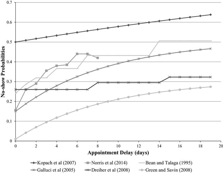
Survey of Patient No‐Show Probabilities

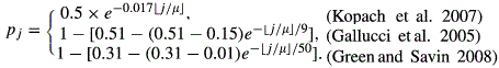
To capture such a wide spectrum of patient no‐show probabilities, we base our numerical experiments below on patient no‐show probabilities reported in Kopach et al. (2007), Gallucci et al. (2005) and the MRI facility of Green and Savin (2008), which represent scenarios of high, medium and low no‐show probabilities, respectively. To be specific, patient show‐up probabilities

p j

in these scenarios are expressed by the following parametric forms (8), where j represents the appointment queue length at patient arrival, μ is the daily service rate and ⌊j/μ⌋ gives the appointment delay in days.

p j = 0.5 × e − 0.017 ⌊ j / μ ⌋ , (Kopach et al. 2007) 1 − [ 0.51 − ( 0.51 − 0.15 ) e − ⌊ j / μ ⌋ / 9 ] , (Gallucci et al. 2005) 1 − [ 0.31 − ( 0.31 − 0.01 ) e − ⌊ j / μ ⌋ / 50 ] . (Green and Savin 2008) .

Comparison of M/M/1/K and M/D/1/K models

In the comparison of M/M/1/K and M/D/1/K models, we use three different sets of patient show‐up probabilities given in Equation 9. We fix the daily service rate μ = 20, but vary the level of demand rate λ ∈ {18,18.5,19,19.5,19.9,19.99} to study the impact of system workload. We consider different combinations of the ancillary task revenue rate ξ and the “rejection” penalty θ. Medical reimbursement data show that ξ is usually smaller than 1. For instance, a 2013 non‐facility Medicare fee for an 11–20 minute phone consultation is $19.25 (CPT code 99442), about one third of that for an office outpatient visit, which costs $53.25 (CPT code 99213). In our experiments, we allow ξ ∈ {0,0.3,0.5}. The parameter θ can be understood as the extra relative cost compared to revenue that the provider would be willing to pay in order to accommodate a patient who would otherwise be rejected. We consider θ ∈ {0,1.0,1.5}, corresponding to three hypothetical cases: the provider is unaffected by rejecting patients due to a full schedule; the provider would be willing to pay an amount equivalent to the revenue generated from serving the patient to avoid a rejection; or the provider would be willing to pay 50% more than an office visit revenue to avoid a rejection. In total, we consider 162 =3 × 6 × 3 × 3 scenarios for each of the two queueing models. Table 1 shows a subset of the optimal appointment queue capacities in these scenarios. We choose not to include results pertaining to ξ = 0.3, θ = 1.0 and λ ∈ {18.5,19.5} because adding these results would not contribute much to the discussion.

OPEN IN VIEWER

Table 1

Comparison Results between the M/M/1/K and M/D/1/K models

(θ,ξ)	λ	K M , K *	K M , G *	K M , G S *	K D , K *	K D , G *	K D , G S *
(0,0)	18	140	60	∞	140	60	∞
	19	80	40	200	80	40	200
	19.9	60	40	80	40	20	60
	19.99	40	40	80	40	20	60
(0,0.5)	18	140	60	∞	140	60	∞
	19	80	40	200	80	40	200
	19.9	60	40	80	40	20	60
	19.99	40	40	80	40	20	60
(1.5,0)	18	∞	200	∞	∞	160	∞
	19	280	100	∞	280	80	500
	19.9	100	60	160	80	40	120
	19.99	100	60	140	80	40	100
(1.5,0.5)	18	∞	∞	∞	∞	∞	∞
	19	540	160	∞	420	160	∞
	19.9	140	80	200	120	60	160
	19.99	140	60	180	100	40	120

The optimal appointment queue capacity is denoted by

K X , Y *

. The subscript X ∈ {M,D} represents the distributional assumption of service times in the queueing model based on which the optimal queue capacity is calculated. The subscript Y ∈ {K,G,GS} indicates the data source of patient show‐up probabilities, which stands for Kopach et al. (2007),Gallucci et al. (2005) and Green and Savin (2008), respectively.

We can make a few important observations here. First, under the M/D/1/K model, the optimal appointment window becomes smaller when the demand rate λ increases with θ and ξ fixed. However, when θ or ξ increases with other parameters fixed, the optimal appointment window gets larger. These are consistent with Proposition 3, proved under the M/M/1/K setting.

In addition, one can numerically verify that according to Condition 1, patients in MRI facilities of Green and Savin (2008) are less sensitive to delays compared to patients in Gallucci et al. (2005). When j ≤ 300 (see Equation 9 for definition of j), sensitivity of patients in Kopach et al. (2007) is higher than that in Green and Savin (2008) but lower than that in Gallucci et al. (2005). Based on this ranking information of patient sensitivity as well as Proposition 2, it is not surprise to see that

K M , G * ≤ K M , K * ≤ K M , G S *

given the same set of λ, ξ and θ. However, a more important observation is that the same ordering results also hold under the M/D/1/K system; that is,

K D , G * ≤ K D , K * ≤ K D , G S *

for fixed λ, ξ and θ. Combined with our discussion above, this verifies that all of our structural results established in the M/M/1/K setting continue to hold under the M/D/1/K Model, at least in the scenarios we tested.

We also note that all the optimal appointment queue capacities are multiples of 20. Recall Corollary 1 which implies that the optimal appointment queue capacity only occurs at the point where patient show‐up probability has a strictly positive decrease. In our case, patient show‐up probabilities drop only at the queue capacities of multiples of 20, the daily service capacity. For example,

p 20 = p 21 = ⋯ = p 39 > p 40

(see Equation 9). Therefore, it is not surprise to see that the optimal appointment queue capacity only takes values like 20,40,60… Indeed, this is a convenient feature for converting the optimal appointment queue capacity into the optimal appointment scheduling window (in days). To do so, one only needs to divide the optimal appointment queue capacity by the daily service capacity, which is 20 in this case, and always gets an integer number of days for the appointment scheduling window.

To examine how “close” an M/M/1/K model approximates an M/D/1/K system in making suggestions for the optimal appointment scheduling window, we note that the M/M/1/K model is able to make exactly the same suggestion as the M/D/1/K model in 28 out of the 72 scenarios we studied. For the rest of 44 cases, we evaluate the efficiency loss in the M/D/1/K Model due to using the optimal appointment window suggested by the M/M/1/K model. Specifically, the efficiency loss is evaluated as

100 % × [ T ( K D * ) − T ( K M * ) ] / T ( K D * )

, where T(·) is the reward function defined in Equation 2 for M/D/1/K systems, and

K M *

and

K D *

, respectively represent the optimal appointment queue capacities calculated based on the M/M/1/K and M/D/1/K settings. The average efficiency loss in these 44 scenarios is only 0.14% and the maximum efficiency loss is 0.97%, suggesting that using the optimal appointment window suggested by the M/M/1/K model in the M/D/1/K model only leads to negligible efficiency loss. Thus, the M/M/1/K model is a fairly accurate approximation for the more realistic M/D/1/K system in terms of suggesting the optimal appointment scheduling window.

Efficiency Gains Resulted from Adopting

K *

In this section, we study how much efficiency gain can be achieved by adopting an optimal appointment scheduling window when practices may or may not use other operational levers.

Cases when Practice Cannot Adjust Panel Size or Overbooking Level

This section deals with the case in which a practice cannot adjust its panel size or overbooking level. Our numerical experiments use similar parameter settings as in section 2. Specifically, we use three different sets of patient no‐show probabilities defined in Equation 9. We fix μ = 20 and vary λ ∈ {18,19,19.9,19.99}, ξ ∈ {0,0.3,0.5} and θ ∈ {0,1.0,1.5}. Different arrival rates λ represent different levels of workload ranging from lightly utilized to extremely congested. We evaluate the efficiency gains based on both M/M/1/K and M/D/1/K Models.

For a given queueing model and a fixed set of parameters, we assess the long‐run average net reward obtained by the system when patients can be scheduled any time into the future, that is, we calculate T(K) defined in Equation 2 for K = ∞. Then, we evaluate the long‐run average net reward when an optimal appointment window is used. That is, we calculate

T ( K * )

in which

K *

is a maximizer to T(K). The efficiency gain is defined as the percentage improvement in long‐run average net reward obtained due to optimizing the appointment scheduling window, that is,

100 % × [ T ( K * ) − T ( ∞ ) ] / T ( ∞ )

. A subset of the representative results are shown in Table 2 (please refer to Table S1 in the Online Appendix for all numerical results).

OPEN IN VIEWER

Table 2

Efficiency Gains Resulted from Adopting

K *

without Other Operational Levers

(θ,ξ)	λ	Δ E M , K (%)	Δ E M , G (%)	Δ E M , G S (%)	Δ E D , K (%)	Δ E D , G (%)	Δ E D , G S (%)
(0,0)	18	0.00	0.00	0.00	0.00	0.00	0.00
	19	0.03	0.46	0.00	0.00	0.06	0.00
	19.9	12.14	21.19	3.02	5.72	13.24	1.40
	19.99	37.71	42.50	9.08	34.84	42.60	8.84
(0,0.5)	18	0.00	0.00	0.00	0.00	0.00	0.00
	19	0.01	0.20	0.00	0.00	0.03	0.00
	19.9	3.65	8.49	1.46	1.81	5.59	0.69
	19.99	9.80	15.41	4.27	9.28	15.65	4.18
(1.5,0)	18	0.00	0.00	0.00	0.00	0.00	0.00
	19	0.00	0.02	0.00	0.00	0.00	0.00
	19.9	8.61	16.67	2.05	3.62	10.26	0.84
	19.99	32.63	36.67	7.71	31.13	38.14	7.84
(1.5,0.5)	18	0.00	0.00	0.00	0.00	0.00	0.00
	19	0.00	0.00	0.00	0.00	0.00	0.00
	19.9	2.02	5.48	0.73	0.81	3.51	0.27
	19.99	7.63	11.82	3.20	7.69	12.87	3.38

Δ E X , Y

is the percentage improvement in long‐run average net reward obtained due to optimizing the appointment scheduling window, that is,

100 % × [ T ( K * ) − T ( ∞ ) ] / T ( ∞ )

. The subscripts X and Y have the same interpretations as those in Table 1.

From Table 2, we find that adopting an optimal appointment scheduling window does not improve efficiency much when patient demand is relatively low compared to daily service capacity (see cases when λ = 18 or 19). However, when patient demand increases, the efficiency gain can be substantial, more than 40% in some cases. To further explore this, we evaluate the probability of a random patient seeing no more than

K *

patients ahead of her upon her arrival to a system with an unlimited appointment scheduling window, that is, a system with K = ∞. Detailed results are presented in Table S2. We note that when patient demand is low, most patients would have an appointment delay shorter than

K *

even when there is no restriction on the appointment window. In other words, most patients are scheduled in the same way as they would be in a system with the optimal appointment window in place. Consequently, restricting the appointment window to be

K *

has limited impact on system efficiency. On the contrary, when patient demand is high, only a small percentage of patients have an appointment delay shorter than

K *

in a system with an unlimited appointment window. As it turns out, adopting an optimal appointment window in this case can effectively reduce appointment delay, control no‐show rates and significantly improve efficiency.

We also note that the efficiency gains become smaller when the “rejection” penalty θ or the ancillary task revenue rate ξ is larger. These observations are in line with what Proposition 3 suggests. As θ or ξ increases,

K *

would also increase and therefore

T ( K * )

gets closer to T(∞) resulting in a smaller efficiency gain. More importantly, we observe that efficiency gains are more sensitive to the changes in ξ than in θ within the range of parameter values we tested. This is likely due to the fact that revenue differentials between patients scheduled in different times are highly sensitive to the value of ξ, and such revenue differentials are the key driver for the optimal choice of appointment scheduling window (see discussions in section 2.2). As ξ increases, these revenue differentials drop quickly, making it less effective to limit the appointment scheduling window.

Cases when Practices May Adjust Panel Size and Overbooking Level

In this section, we consider the cases in which practices can adjust their panel size and overbooking level freely. We adopt the same three sets of patient no‐show probabilities as above, and vary θ ∈ {0,1.0,1.5} and ξ ∈ (0,0.3,0.5) in our experiments. We consider both the M/M/1/K and M/D/1/K queueing models. Given a queueing model and a fixed parameter setup, we assume that the practice first optimizes its panel size and overbooking level following the model of Liu and Ziya (2014), which we briefly recapitulate below. In particular, the practice solves the following optimization problem first.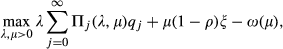

max λ , μ > 0 λ ∑ j = 0 ∞ Π j ( λ , μ ) q j + μ ( 1 − ρ ) ξ − ω ( μ ) ,

where λ and μ are decision variables representing the demand rate (panel size) and service rate (overbooking level) in the system, respectively. The variable ρ = λ/μ is the traffic intensity, and

Π j ( λ , μ )

represents the steady state probability that an incoming patient sees j patients ahead upon her arrival for a given pair of λ and μ. Note that the objective function above is essentially a special case of Equation 2 with K = ∞ minus the last term ω(μ), which represents the cost of providing the service. We adopt the form

ω ( μ ) = a × [ ( μ − M ) + ] 2

from Liu and Ziya (2014) in our experiments, and set the regular daily capacity M = 20 patients per day and the overtime cost parameter a ∈ {0.2,2}. Thus, if the practice chooses μ to be larger than 20, it overbooks μ − 20 patients and incurs overtime cost ω(μ) per day.

After the practice solves the optimization problem (9) above and obtains the optimal patient demand rate

λ *

and daily service capacity

μ *

, it seeks the optimal appointment window

K *

given

( λ * , μ * )

. We evaluate the percentage efficiency gains resulted from further adopting an optimal scheduling window in systems with the already optimized panel size and overbooking level. As it turns out, when the overtime cost parameter a = 2, the practice never overbooks, that is, it always set

μ * = M = 20

. In this case, we can think of the practice does not have an overbooking option (due to its high overtime cost) but can freely adjust its panel size. Table 3 shows a subset of the representative results and full results appear in Table S3.

OPEN IN VIEWER

Table 3

Performance Results of Adopting

K *

with Other Operational Levers

(θ,ξ)	No‐show model	( K * , λ * , μ ) vs. ( ∞ , λ * , μ )				( K * , λ * , μ * ) vs. ( ∞ , λ * , μ * )
		Δ E M (%)	α M	Δ E D (%)	α D	Δ E M (%)	α M	Δ E D (%)	α D
(0,0)	K	0.29	0.86	0.16	0.86	0.64	0.80	0.50	0.77
	G	0.97	0.81	0.43	0.73	0.81	0.84	0.85	0.68
	GS	0.29	0.80	0.06	0.92	0.15	0.87	0.20	0.86
(0,0.5)	K	0.09	0.86	0.05	0.86	0.17	0.82	0.12	0.80
	G	0.43	0.81	0.19	0.73	0.36	0.84	0.38	0.68
	GS	0.14	0.80	0.03	0.92	0.07	0.87	0.10	0.86
(1.5,0)	K	0.00	1.00	0.00	1.00	0.04	0.99	0.04	0.99
	G	0.13	0.96	0.06	0.98	0.09	0.97	0.16	0.97
	GS	0.05	0.96	0.00	1.00	0.01	0.99	0.04	0.97
(1.5,0.5)	K	0.00	1.00	0.00	1.00	0.00	1.00	0.00	1.00
	G	0.00	1.00	0.00	1.00	0.00	1.00	0.02	0.99
	GS	0.00	0.99	0.00	1.00	0.00	1.00	0.00	0.99

Δ E X

and

α X

represent the percentage efficiency gain and the service level, respectively. The service level is defined as the probability of patients seeing no more than

K *

patients ahead upon their arrivals to a system with the optimal panel size (and optimal overbooking level) but an infinite appointment scheduling window. The symbols K, G and GS as well as the subscript X ∈ {M,D} have the same interpretation as those in Table 1. The third grand column, in which μ = 20, presents the cases without an overbooking option.

From Table 3, we observe that once the panel size (and the overbooking level) is optimized, the efficiency gains by further adopting an optimal appointment scheduling window are limited (less than 1% in all scenarios). To explain this, we evaluate based on both queueing models, the service level defined as the probability of patients seeing no more than

K *

patients ahead upon their arrivals to a system with the optimal panel size (and optimal overbooking level) but an infinite appointment scheduling window.

K *

is the optimal appointment scheduling window that could be set given that the optimal panel size (and overbooking level) is already in place. As we see in Table 3, these service levels are at least 68%, suggesting that optimizing the panel size (and the overbooking level) can already control patient appointment delay (and patient no‐show rates) quite well. Further setting a limit on the appointment window seeks to achieve a similar goal of influencing appointment delays experienced by patients, and thus can only exert a limited impact.

Efficiency Gains Due to Jointly Optimizing All Operational Levers

To further explore the efficiency gain by controlling the appointment scheduling window, we consider cases when practices can jointly optimize all operational levers: panel size, overbooking level and appointment scheduling window. Specifically, the practice solves the following optimization problem.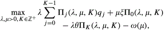

max λ , μ > 0 , K ∈ Z + λ ∑ j = 0 K − 1 Π j ( λ , μ , K ) q j + μ ξ Π 0 ( λ , μ , K ) − λ θ Π K ( λ , μ , K ) − ω ( μ ) ,

in which

Π j ( λ , μ , K )

represent the steady‐state queue length for a given triplet of (λ,μ,K). We adopt the same three sets of patient no‐show probabilities as above, and vary θ ∈ {0,1.0,1.5}, ξ ∈ (0,0.3,0.5) and a ∈ {0.2,2} in our experiments. For convenience, we let

( K * * , λ * * , μ * * )

represent the jointly optimal scheduling window, panel size and overbooking level to (10). We evaluate the percentage efficiency gains due to using

( K * * , λ * * , μ * * )

compared with using

( K * , λ * , μ * )

obtained in section (3.3.2) (see detailed results in Table S4). Except for the cases when θ = 0, the efficiency gains due to joint optimization are almost zero. When θ = 0, that is, when providers are not affected by “rejecting” patients due to a full schedule, the jointly optimal strategy appears to be using a very large panel (ideally containing an infinite number of patients) and adopting a very small appointment window (ideally one day), so that there are always patients in the system whose appointment delay is minimal yielding the maximal possible revenues. Even with such an unrealistic strategy, the M/D/1/K Model estimates that the largest efficiency gain is no more than 5% in all cases we tested. Therefore, taking together with our previous numerical results, we may conclude that optimizing the appointment scheduling window serves more as a substitute, rather than a complement, to optimizing the panel size (and overbooking level).

Extension to Heterogeneous Customers

The previous sections deal with models with homogeneous customers. However, customers with different personal characteristics may differ in their no‐show probabilities. For instance, patients who had missed their prior appointments tend to have a higher chance of breaking their future appointments (Norris et al. 2014). Observing this phenomenon, providers may use different appointment windows for patients depending on their no‐show behaviors (D. Rosenthal 2011, Columbia University, pers. comm., DuMontier et al. 2013). In this section, we consider a simple stylized model with heterogeneous customers to study such decision making. In particular, we assume that there are two types of patients who differ in their arrival rates and show‐up probabilities. Type i patients join the queue according to a Poisson process with rate

λ i

for i = 1,2. The probability that a type i patient will show up given j patients ahead of her upon her appointment request is

p i j

. Similar to our previous models, we assume that these show‐up probabilities decrease as patient appointment delay increases, that is,

p i j ≥ p i , j + 1

for i = 1,2 and j = 0,1,2,…. We also assume that the provider knows exactly the patient type when a patient arrives, and she may use patient type‐specific appointment windows. That is, the provider will not schedule type i patients if there are already

K i

patients (regardless of their types) in the system, where

K 1

can be different from

K 2

.

Except for the differences above, these two types of customers are the same in other aspects and model assumptions are also similar to those of the M/M/1/K model with homogeneous customers considered in section 2. The service times of each customer are i.i.d. exponential random variables with mean 1/μ. If the scheduled customer does not show up for an appointment slot or there is no customer scheduled for that slot, the provider is able to fill it by an ancillary task which yields a reward ξ ∈ [0,1). Each patient served brings in one nominal unit of reward and each unscheduled patient incurs a cost θ to the system. The provider's objective is to maximize the long‐run average net reward by choosing

K 1

and

K 2

appropriately.

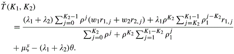
One can show that for this stylized model, the long‐run average net reward given

( K 1 , K 2 )

, denoted as

T ( K 1 , K 2 )

, has a closed‐form expression. To be specific, let

ρ = ( λ 1 + λ 2 ) / μ

,

ρ i = λ i / μ

,

w i = λ i / ( λ 1 + λ 2 )

, and

r i j = θ + ( 1 − ξ ) p i j

for i = 1,2, and j = 0,1,2,…. We need to consider two cases separately:

K 2 ≥ K 1

and

K 1 > K 2

. We use

T ( K 1 , K 2 | K 2 ≥ K 1 )

to represent the long‐run average net reward collected by the system given that

K 2 ≥ K 1

, that is, when the service provider allows a longer appointment scheduling window for type 2 customers. For convenience, we write

T ^ ( K 1 , K 2 ) = T ( K 1 , K 2 | K 2 ≥ K 1 )

. Similarly, we write

T ( K 1 , K 2 | K 1 ≥ K 2 )

as

T ˇ ( K 1 , K 2 )

. Then, by modeling the number of scheduled appointments in the system as a Continuous Time Markov Chain for each of the two cases, we can obtain the following expressions for

T ^ ( K 1 , K 2 )

and

T ˇ ( K 1 , K 2 )

, respectively. Detailed derivations are presented in Appendix S2.

T ^ ( K 1 , K 2 ) = ( λ 1 + λ 2 ) ∑ j = 0 K 1 − 1 ρ j ( w 1 r 1 , j + w 2 r 2 , j ) + λ 2 ρ K 1 ∑ j = K 1 K 2 − 1 ρ 2 j − K 1 r 2 , j ∑ j = 0 K 1 ρ j + ρ K 1 ∑ j = 1 K 2 − K 1 ρ 2 j + μ ξ − ( λ 1 + λ 2 ) θ ,

and

T ˇ ( K 1 , K 2 ) = ( λ 1 + λ 2 ) ∑ j = 0 K 2 − 1 ρ j ( w 1 r 1 , j + w 2 r 2 , j ) + λ 1 ρ K 2 ∑ j = K 2 K 1 − 1 ρ 1 j − K 2 r 1 , j ∑ j = 0 K 2 ρ j + ρ K 2 ∑ j = 1 K 1 − K 2 ρ 1 j + μ ξ − ( λ 1 + λ 2 ) θ .

Now we can evaluate the long‐run average net reward

T ( K 1 , K 2 )

for any

( K 1 , K 2 )

using

T ( K 1 , K 2 ) = T ˇ ( K 1 , K 2 ) if K 1 > K 2 , T ^ ( K 1 , K 2 ) if K 2 ≥ K 1 .

And the service provider's problem can be formulated as

max K 1 , K 2 ∈ Z + T ( K 1 , K 2 ) .

P2

As discussed earlier, the service provider may either use the same appointment window for them, or differentiate the appointment windows based on patient type. Below we consider these two cases separately.

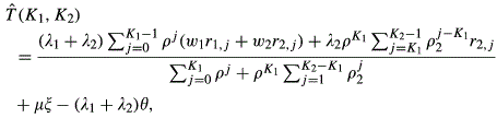
Case that Requires K₁ = K₂

When the service provider choose to use the same appointment window, she simply sets

K 1 = K 2

as a constraint in problem (P2). The arrivals of both types of patients follow independent Poisson processes with rates

λ 1

and

λ 2

, respectively. Thus, the joint arrival process is also a Poisson process, with rate

λ 1 + λ 2

. The probability that an arriving patient belongs to type i is

w i

(see Theorem 5.6 in Kulkarni 1995). Therefore, for a random arrival who sees j patients ahead of her, her expected show‐up probability is

p ¯ j = w 1 p 1 j + w 2 p 2 j

, j = 0,1,2,…. When

K 1 = K 2

, the number of patients registered in the system becomes an

M / M / 1 / K 1

queue. In this case, the model with heterogeneous customers simply reduces to a model with homogeneous customers where λ and

p j

are replaced by

λ 1 + λ 2

and

p ¯ j

, respectively. Therefore, all results derived in section 2 apply to this case.

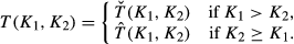
Case that Allows K₁≠ K₂

When the provider can freely choose appointment windows, intuition suggests that the provider would be better off by offering a longer appointment scheduling window for customers who have higher show‐up probabilities, because these “better behaved” customers can be held longer in the system while still having the same or higher show‐up probabilities. Indeed, such a scheduling paradigm is widely adopted in practice to deal with frequent no‐show offenders by offering them very short appointment windows (see D. Rosenthal 2011, Columbia University, pers. comm., DuMontier et al. 2013). However, we have seen that the intuition above fails when customers are homogeneous (or equivalently, when the provider does not know the patient type information but can only treat every patient as a random draw from a patient population with a common no‐show probability distribution). In that case, solely improving customer show‐up rates does not guarantee a larger appointment scheduling window to be optimal (see Example 1). Customer sensitivity to delays plays a more important role there. Could customer sensitivity to delay play a similar role when customers are heterogeneous in their no‐show behavior and the provider knows exactly their type?

The following proposition provides some answer to the question above. It actually points to a different result to the homogeneous case. When patients are heterogenous and the provider knows exactly their type, it would be optimal for the provider to set a longer appointment window for patients with higher show‐up probabilities, irrespective of their sensitivity to delays.

Proposition 4

If

p 1 j ≤ p 2 j

for j = 0,1,2,…, then there exists an optimal pair of the appointment queue capacities

( K 1 * , K 2 * )

such that

K 1 * ≤ K 2 *

.

To give an intuitive explanation for Proposition 4, imagine that the provider sets an appointment window

K 1

for type 1 patients who have lower show‐up probabilities. Suppose that at this moment, the queue length is shorter than

K 1

. If a type 1 patient arrives, the provider would accept this patient to the system. If instead a type 2 patient comes at this moment, the provider seems to have no reason to “reject” this patient as this patient has a higher show‐up probability than type 1 patients. Following this logic, the provider should set

K 2

at least the same as

K 1

.

In the proposition above,

p 1 j ≤ p 2 j

is the only required condition for this ordering result to hold. It actually holds independently of all other model parameters, such as customer arrival rates

λ 1

and

λ 2

and provider service rate μ. Put into the context of health care management, Proposition 4 gives a robust ordering result that does not depend on patient mix or practice size, indicating that as long as one group of patients have higher show‐up rates, allowing a longer appointment window for them can lead to better system performance.

Conclusion

Patients’ no‐show behavior presents a significant problem faced by many health care providers. Since patient no‐show rates usually increase with their appointment delays, one commonly‐adopted operational strategy by providers is to control the length of the appointment window. By limiting patients from making appointments too far away into the future, the provider reduces patient appointment delays and thus no‐show rates. Although there is a growing body of literature on various operational strategies to deal with patient no‐shows, little is known about the impact of varying appointment scheduling windows on a provider's operational efficiency. This study is directed to fill this knowledge gap.

The key trade‐off here is between the efficiency loss due to high no‐show rates following from allowing a longer appointment window and the “penalty” resulted from an overly restrictive appointment window driving too many patients unable to schedule their appointments. We capture this trade‐off by using a single server queue to model the appointments registered in a provider's work schedule. The capacity of the queue serves as a proxy of the length of the appointment window. The provider wants to set a common appointment window for all patients, who have higher no‐show probabilities when their appointment delays are longer, to maximize her long‐run average net reward. Using a stylized M/M/1/K queueing model, we provide analytical characterizations for the optimal appointment queue capacity, and study how the optimal scheduling window should be adjusted in response to changes in other model parameters. Through extensive numerical experiments, we confirm that our analytical results continue to hold in more realistic settings. In addition, one particularly useful message from our numerical study to practitioners is that adopting an optimal appointment scheduling window can lead to substantial efficiency gains if the provider has no other operational levers at hand to deal with patient no‐shows. However, when the provider can adjust panel size and overbooking level, limiting the appointment scheduling window serves more as a substitute strategy, rather than a complement.

Our work points to several directions for future research. First, our model extension studies a single server queue with two types of patients differing in their no‐show probabilities. The provider knows the type of each incoming patient, and may set different appointment windows depending on patient type. These patient type‐specific appointment windows, however, are static over time and independent of the system state. A dynamic admission policy which depends on the current patient composition in the queue or a policy that sets a limit on the number of each type of patients in the system holds the promise of further improving system efficiency. However, these variations would lead to completely different and likely more challenging optimization problems, which we leave for future research. Second, in our model with heterogeneous patients, we assume that providers can perfectly segment patients based on their no‐show probabilities. However, misclassification errors may occur in reality and it is important to study how such errors can affect our analysis and results. Third, our model is stylized in nature mainly for deriving managerial insights and more research is needed to develop decision support tools for practical use. For example, patients may have stronger preferences for convenient times of day rather than shorter appointment delays, and thus they may not accept the earliest available appointment. In addition to no‐shows, patients may cancel in advance or reschedule their appointments. These patient behaviors can leave “holes” in the appointment queue. In this case, a first‐come‐first‐served queue may not be an accurate representation. Thus, one avenue for future research is to examine the connection between the appointment window size and the operational efficiency in a more realistic setting. Analytical study based on stylized queueing models may be difficult, but simulation experiments are likely to yield useful results.

Footnotes

Acknowledgments

The author is grateful to the departmental editor, the senior editor and the anonymous referees, whose comments and suggestions have helped improve this work. The author also thanks the audience at the workshop on Data‐Driven Decisions in Healthcare, organized by the Statistical and Applied Mathematical Sciences Institute (SAMSI) in 2013 for their useful feedback. This work was partially supported by the Calderone Junior Faculty Research Award, Mailman School of Public Health, Columbia University.

References

1.

Atun R. A. Sittampalam S. R. Mohan A. . 2005. Uses and benefits of SMS in healthcare delivery. Working paper, Tanaka Business School, Imperial College.

Go to Reference

2.

Bean A. G. Talaga J. . 1995. Predicting appointment breaking. J. Health Care Mark. 15(1): 29–34.

Go to Reference

3.

Cayirli T. Veral E. . 2003. Outpatient scheduling in health care: A review of literature. Prod. Oper. Manag. 12(4): 519–549.

Go to Reference

4.

Dreiher J. Froimovici M. Bibi Y. Vardy D. A. Cicurel A. Cohen A. D. . 2008. Nonattendance in obstetrics and gynecology patients. Gynecol. Obstet. Invest. 66(1): 40–43.

+ Show References

5.

DuMontier C. Rindfleisch K. Pruszynski J. Frey J. J. III. 2013. A multi‐method intervention to reduce no‐shows in an urban residency clinic. Fam. Med. 45(9): 634–641.

+ Show References

6.

Gallucci G. Swartz W. Hackerman F. . 2005. Brief reports: Impact of the wait for an initial appointment on the rate of kept appointments at a mental health center. Psychiatr. Serv. 56(3): 344–346.

+ Show References

7.

Geraghty M. Glynn F. Amin M. Kinsella J. . 2007. Patient mobile telephone text reminder: A novel way to reduce non‐attendance at the ENT out‐patient clinic. J. Laryngol. Otol. 122(3): 296–298.

+ Show References

8.

Green L. V. Savin S. . 2008. Reducing delays for medical appointments: A queueing approach. Oper. Res. 56(6): 1526–1538.

+ Show References

9.

Gupta D. Denton B. . 2008. Appointment scheduling in health care: Challenges and opportunities. IIE Trans. 40(9): 800–819.

Go to Reference

10.

Guy R. Hocking J. Wand H. Stott S. Ali H. Kaldor J. . 2012. How effective are short message service reminders at increasing clinic attendance? A meta‐analysis and systematic review. Health Serv. Res. 47(2): 614–632.

Go to Reference

11.

Hashim M. J. Franks P. Fiscella K. . 2001. Effectiveness of telephone reminders in improving rate of appointments kept at an outpatient clinic: A randomized controlled trial. J. Am. Board Fam. Pract. 14(3): 193–196.

Go to Reference

12.

Hassin R. Mendel S. . 2008. Scheduling arrivals to queues: A single‐server model with no‐shows. Manage. Sci. 54(3): 565–572.

Go to Reference

13.

Kopach R. DeLaurentis P. C. Lawley M. Muthuraman K. Ozsen L. Rardin R. Wan H. Intrevado P. Qu X. Willis D. . 2007. Effects of clinical characteristics on successful open access scheduling. Health Care Manage. Sci. 10(2): 111–124.

+ Show References

14.

Kulkarni V. G. 1995. Modeling and Analysis of Stochastic Systems. Chapman & Hall/CRC, Boca Raton, FL.

+ Show References

15.

LaGanga L. R. Lawrence S. R. . 2007. Clinic overbooking to improve patient access and increase provider productivity. Decis. Sci. 38(2): 251–276.

Go to Reference

16.

Liu N. Ziya S. . 2014. Panel size and overbooking decisions for appointment‐based services under patient no‐shows. Prod. Oper. Manag. 23(12): 2209–2223.

+ Show References

17.

Liu N. Ziya S. Kulkarni V. G. . 2010. Dynamic scheduling of outpatient appointments under patient no‐shows and cancellations. Manufac. Serv. Oper. Manag. 12(2): 347–364.

+ Show References

18.

Macharia W. M. Leon G. Rowe B. H. Stephenson B. J. Haynes R. B. . 1992. An overview of interventions to improve compliance with appointment keeping for medical services. J. Am. Med. Assoc. 267(13): 1813–1817.

Go to Reference

19.

Merrell K. Berenson R. A . 2010. Structuring payment for medical homes. Health Aff. 29(5): 852–858.

Go to Reference

20.

Moore C. G. Wilson‐Witherspoon P. Probst J. C. . 2001. Time and money: Effects of no‐shows at a family practice residency clinic. Fam. Med. 33(7): 522–527.

Go to Reference

21.

Murray M. Tantau C. . 2000. Same‐day appointments: Exploding the access paradigm. Fam. Pract. Manag. 7(8): 45–50.

Go to Reference

22.

Muthuraman K. Lawley M. . 2008. A stochastic overbooking model for outpatient clinical scheduling with no‐shows. IIE Trans. 40(9): 820–837.

Go to Reference

23.

Nguyen D. L. DeJesus R. S. Wieland M. L. . 2011. Missed appointments in resident continuity clinic: Patient characteristics and health care outcomes. J. Grad. Med. Educ. 3(3): 350–355.

Go to Reference

24.

Norris J. B. Kumar C. Chand S. Moskowitz H. Shade S. A. Willis D. R. . 2014. An empirical investigation into factors affecting patient cancellations and no‐shows at outpatient clinics. Decis. Support Syst. 57: 428–443.

+ Show References

25.

Patrick J. Puterman M. L. Queyranne M. . 2008. Dynamic multi‐priority patient scheduling for a diagnostic resource. Oper. Res. 56(6): 1507–1525.

Go to Reference

26.

Robinson L. W. Chen R. R. . 2010. A comparison of traditional and open‐access policies for appointment scheduling. Manufac. Serv. Oper. Manag. 12(2): 330–346.

Go to Reference

27.

Rural Assistance Center . 2013. Federally Qualified Health Centers frequently asked questions. Available at http://www.raconline.org/topics/federally-qualified-health-centers/faqs (accessed date August 9, 2014).

Go to Reference

28.

Schectman J. M. Schorling J. B. Voss J. D. . 2008. Appointment adherence and disparities in outcomes among patients with diabetes. J. Gen. Intern. Med. 23(10): 1685–1687.

Go to Reference

29.

Shin P. Sharac J. Alvarez C. Rosenbaum S. . 2013. Community health centers in an era of health reform: An overview and key challenges to health center growth executive summary. The Kaiser Commission on Medicaid and the Uninsured, March 2013.

Go to Reference

30.

U.S. Department of Health and Human Services . 2014. What are Federally qualified health centers (FQHCs)? Available at http://www.hrsa.gov/healthit/toolbox/RuralHealthITtoolbox/Introduction/qualified.html (accessed date August 9, 2014).

Go to Reference

31.

Zeng B. Turkcan A. Lin J. Lawley M. . 2010. Clinic scheduling models with overbooking for patients with heterogeneous no‐show probabilities. Ann. Oper. Res. 178(1): 121–144.

Go to Reference