Traffic‐Based Labor Planning in Retail Stores

Introduction

Effective management of store labor is important to successful retail operations as store labor performs all service‐related tasks (e.g., check‐out, returns, shopping assistance) (Fisher et al. 2006), production‐like tasks (i.e., in‐store logistics) (Fisher 2004, Ton 2009) and labor costs are among the largest costs retailers incur in day‐to‐day operations. The retail environment is characterized by volatile store traffic, which complicates the process of determining staffing levels and affects retailers’ ability to provide consistent service quality. Therefore, the ability to match store labor with incoming customer traffic in an efficient manner is a critical driver of retailers’ store performance. In this study, we explore the relationship among sales, labor, and traffic. The exploration prompted development of a heuristic that enables retailers to use customer traffic patterns to determine their labor requirements.

Traditional staffing practices in retailing are primarily sales‐driven and depend on store budget allocation. A typical sales‐based staffing rule is to match a constant ratio of expected store sales to the number of store associates [refer to Lam et al. (1998, p. 62) for a detailed discussion of traditional staffing practices]. A staffing policy primarily driven by sales, however, ignores the fact that retail sales are also affected (among other factors) by store traffic and might result in labor‐to‐traffic‐mismatches, which can have a negative impact on sales revenue (Netessine et al. 2010, Perdikaki et al. 2012). Retailers cannot fully exploit their sales potential if they follow such staffing policies because the scheduled labor may not be enough to accommodate customer traffic flows. In addition, latent shopper demand may be very different from past sales, since past sales include only customers who purchased and not those who had an intention to purchase but left the store due to lack of sales associate assistance. The proportion of customers who typically leave a store because of poor service is not negligible. Extensive interviews with American customers reveal that “33% who experienced a problem could not find sales help when they required assistance. At the end of the day 6% of all shoppers are lost due to lack of sales associate availability” (Baker Retail Initiative 2007, p. 3). Inevitably, such staffing practices have negative short‐term and long‐term implications for retail store performance.

Recently, retailers have been making better use of information available at the store level to improve traditional staffing practices. Specifically, retailers invest heavily in different types of in‐store technology such as sales‐tracking systems, workforce‐planning systems, and traffic‐counting systems to ensure that stores are staffed with the right number of sales associates. Utilizing such technologies enables retailers to generate traffic forecasts for their stores and consider several store specific characteristics to determine the aggregate labor hours required for each store. Even though this approach is an improvement from traditional labor‐planning practices that rely mainly on sales forecasts, it has a strong focus on within‐store performance. Going beyond the focus on individual stores, retailers could better leverage the information available to them by also considering the performance across different stores in their retail chains. In this study, we present an approach that enables retailers to derive aggregate labor requirements by utilizing traffic data, point‐of‐sale (POS) data, and labor data across stores with similar attributes (e.g., store format, product mix, and market demographics). We show that such an approach leads to robust performance while identifying average differences across stores in the chain.

We analyze proprietary data on labor, traffic, and sales collected from 46 stores of a high‐end women's apparel retailer. We investigate the apparel sector because, unlike other retail settings (e.g., grocery stores) that have a close to 100% conversion rate of turning shoppers into buyers (Netessine et al. 2010), apparel stores exhibit considerable heterogeneity in conversion rates and thus staffing levels have a stronger influence on converting traffic into sales (Perdikaki et al. 2012). Our modeling effort focuses on panel data to leverage the between‐store variation in sales, traffic, and labor in addition to the within‐store temporal variation used by existing staffing approaches (e.g., Kabak et al. 2008, Lam et al. 1998). We develop a sales response function with the appropriate characteristics to make reliable staffing decisions and demonstrate that the function has strong explanatory power of sales variation. Using the estimated parameters of the sales response function, we formulate a profit‐maximizing problem and propose a traffic‐based heuristic to help managers determine weekly staffing levels. We assess the performance of the heuristic's staffing recommendations by performing counterfactual experiments (Kydland and Prescott 1996), and find that the heuristic performs close to the optimal based on the sales response function, and generates higher profits than the observed staffing levels.

While our study is not the first in the literature that proposes a traffic‐based labor‐planning approach, our study makes improvements in the following dimensions. First, we formulate a sales response function based on labor adequacy (the ratio of labor to traffic) that exhibits the expected variable elasticity of substitution between traffic and labor in the retail space—while it might be easy to maintain a level of sales by bringing in additional traffic to replace lost labor when the staffing levels are adequate, increasing store traffic should not have as high of an impact when labor is already utilized to capacity. Second, we employ panel estimation methods—widely used fixed effects modeling as well as recently promoted random effects modeling with Mundlak's correction (Bell and Jones 2015, Mundlak 1978)—that allow us to leverage information available from the performance across stores, as opposed to just the within‐store performance variability, resulting in much more efficient and robust estimates for our sales function. We show that our proposed sales response function exploits the information content from the fit sample more effectively and predicts sales under extreme input conditions better than the function in related literature. Furthermore, the proposed formulation and estimation could potentially allow management to isolate time‐invariant store differences that affect the stores’ ability to turn traffic into sales. Third, we use the sales function to develop a data‐driven staffing heuristic that incorporates the prediction loss function (Granger 1969, West 1996) and uses past traffic to predict optimal labor, as opposed to attempting to forecast volatile traffic. The optimal labor prediction yields staffing levels that are commensurate to other stores’ staffing levels as opposed to levels that are just continuation trends of a store's current practices. In counterfactual experiments, we show that the heuristic achieves profits that are within 0.5% of the optimal (attainable if perfect traffic information was available) under stable traffic conditions and within 2.5% of the optimal under extreme traffic variability.

The rest of this article is organized as follows. Section 2 summarizes the relevant literature; Section 3 describes the research setting and the panel data used for analysis. In section 4, we propose a sales response function, discuss its theoretical properties, and present estimation results of the function. In section 5, we present a traffic‐based staffing heuristic and in section 6 we assess its performance and conduct sensitivity analyses. We conclude by discussing managerial implications of our findings and potential extensions of our work.

Related Literature

Labor planning has been a traditional area of research in operations management and a large body of literature has focused on mathematical modeling to facilitate labor‐planning decisions. The emerging stream of empirical research on retail labor management is primarily motivated by Raman et al. (2001) who posit that store labor is key to resolving execution issues such as inventory record inaccuracy (DeHoratius and Raman 2008) and phantom stockouts (Ton and Raman 2010). Fisher et al. (2006) examine the impact of execution issues on customer satisfaction and sales and propose labor reallocation across stores to enhance sales. Since experienced store associates are usually more capable of executing prescribed tasks correctly, one critical issue of retail labor management is to reduce employee turnover and the associated loss of accumulated experience (Cascio 2006). Ton and Huckman (2008) find employee turnover is negatively associated with profit margin and customer service in a US retail chain. Because high employee turnover is often caused by working overtime, pressure, and fatigue, increasing staffing levels is an effective way to relieve workload and enhance service quality (Oliva and Sterman 2001). In addition to the well‐known effect of labor on service quality, Ton (2009) finds that increasing the amount of labor leads to profit increases through labor effects on conformance quality and Chuang and Oliva (2015) find a positive impact of staffing levels and labor‐mix on inventory data quality. Netessine et al. (2010) examine the impact of labor planning and labor execution on store performance and find that matching store labor to traffic is associated with greater basket values. Their study, which does not possess actual traffic data but uses monthly data on the number of transactions as a proxy for traffic, suggests that better labor planning and execution would lead to superior store performance. Our study is different from the above descriptive body of literature in its research question and data. We study labor together with actual store traffic to develop a traffic‐based labor‐planning heuristic for retail environments.

While the impact of labor on retail performance has been extensively analyzed in the aforementioned studies, traffic has been comparatively understudied because of the difficulty to measure and record actual store traffic. Few studies obtain actual traffic data to assess the effect of traffic and labor on store performance (Perdikaki et al. 2012) and utilize such data to improve/support store labor‐planning decisions (Kabak et al. 2008, Lam et al. 1998, Mani et al. 2015). Lam et al. (1998) propose a sales response function‐relating store sales to traffic and labor and use traffic forecasts to plan labor in a single store. Kabak et al. (2008) adopt Lam et al.'s function to determine hourly staffing requirements, which are used as inputs of a mixed integer program to optimize daily shifts. Our study differs from Kabak et al. (2008) in that their staffing requirements are based on forecasted sales revenue as opposed to store traffic. In addition, while Kabak et al. (2008) focus on optimizing the hourly labor plan, given the sales forecast, our goal is to develop a methodology that effectively uses traffic information to perform weekly labor allocation. Mani et al. (2015) provide a methodology that identifies the extent of understaffing in retail stores and its impact on sales and profitability. Our study is different from Mani et al.'s (2015) in the following dimensions. Mani et al.'s (2015) objective is to develop a methodology to assist labor planning by identifying periods during the day where overstaffing and understaffing occur. We, on the other hand, view planning at a higher level and are interested in determining the aggregate requirements of labor hours at a store on a weekly level. Moreover, the optimal staffing rule proposed by Mani et al. (2015) is technically more complicated in that it requires imputation of unobserved labor costs. Although econometricians do not typically have access to employee wages, store managers have labor cost information when making their staffing decisions. Thus, our heuristic, which does not require labor cost imputation, is easier for retailers to implement. Finally, Perdikaki et al. (2012) empirically examine how traffic and labor affect store performance. They find that sales exhibit diminishing returns to scale with respect to traffic; labor moderates the impact of traffic on sales; and conversion rate declines with increasing traffic. Our objective differs from Perdikaki et al.'s (2012) in that we are interested in providing a framework to support store labor‐planning decisions. To that end, we propose and assess the performance of a simple heuristic using counterfactual experimentation.

Our study is closest to Lam et al. (1998) who propose a traffic‐based labor‐planning methodology based on traffic forecast. We improve on their paper in three important ways. First, we develop a formulation and estimation method that allows us to leverage information across multiple stores and utilize the performance variability across stores. Second, our sales response function is based on labor adequacy (the ratio of labor to traffic) and exhibits variable elasticity of substitution between traffic and labor. From an information theory perspective, our sales response function exploits the information content from the fit sample more effectively than Lam et al.'s. Finally, unlike Lam et al.'s (1998) labor‐planning approach that relies on traffic forecast, we propose an approach that exploits only past traffic information and still performs within 2.5% of the optimal even under extreme traffic conditions.

Research Setting and Data Description

Our research site is a large US retail chain that specializes in women's high‐end fashion apparel. As of 2013, the retailer had more than 200 stores located in the United States, the District of Columbia, Puerto Rico, the U.S. Virgin Islands, and Canada. The retailer's stores are located mainly in shopping centers and malls.

The retailer had installed customer traffic counters in 60 of its US stores during our study period. Those traffic counters were purchased from a company that develops advanced traffic counting systems and guarantees a very high percentage of performance accuracy. This technology has several capabilities such as counting groups of people; distinguishing between incoming and outgoing customer traffic; and differentiating between adults and children, while not counting shopping carts or strollers. This traffic counting system also responds well to different levels of light in the store and can prevent certain types of counting errors such as customers entering but immediately exiting the store.

We obtained the following daily data for the retailer over a whole calendar year (52 weeks): (i) store sales volume (total revenue in $), (ii) labor data (employee hours), and (iii) traffic data (total number of customers). The stores were open 7 days a week and their operating hours were different among locations and days of the week, for example, weekends and weekdays. Out of 60 stores, there were nine stores for which we did not have traffic information for the entire 52 weeks. Those stores had either opened later during that year or had not installed traffic counters at the beginning of the year. Moreover, there were five stores that were in malls that did not have a working website so we could not obtain their operating hours. Thus, we restricted our analysis to the remaining 46 stores for which we could obtain complete information with respect to our variables of interest.

The retailer uses a proprietary labor‐planning system to perform in‐store labor allocation. The tool is run centrally (i.e., at corporate headquarters), and provides weekly labor requirements to store managers who use this information as an input to make more detailed staffing scheduling decisions (i.e., day‐by‐day and hour‐by‐hour), taking different constraints into account such as employees’ preferred schedules and vacations.

While the data were available on a daily basis, we analyzed weekly labor capacity following Oliva and Sterman (2001) and Siebert and Zubanov (2010). Although we also check the effectiveness of our analysis based on a daily data aggregation (see subsection 4.3), several structural elements better justify the weekly data aggregation. First, the weekly aggregation is consistent with staffing planning practices in the apparel retail sector that determines weekly capacity requirements and later decides on day‐to‐day scheduling decisions (Pastor and Olivella 2008). Second, this approach is also consistent with this retailer's labor planning practices. Weekly labor requirements are provided as a recommendation to local store managers by the centralized labor‐planning system, while detailed workforce scheduling decisions (e.g., day‐by‐day, hour‐by‐hour) are more appropriate for local store managers who have better knowledge about constraints pertaining to local contracts and labor availability. Finally, the fraction of a store's weekly traffic that occurs in any given day of the week does not vary much for each store (e.g., 15% of the week's traffic occurs on Friday, 10% on Mondays, etc.) and explains 70% of the variation of sales within a week, making the translation from weekly labor requirements to daily requirements a simple exercise, again, best informed by the local store constraints.

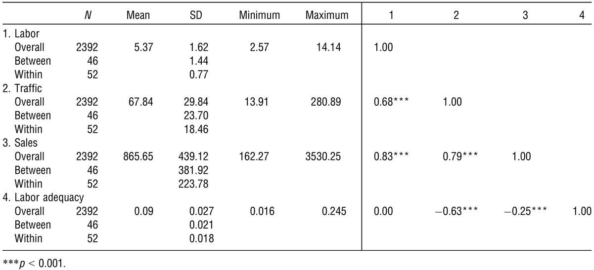
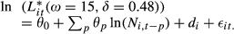
As discussed earlier, the stores’ operating hours were different among locations and days of the week. To avoid any potential spurious correlation that could arise due to systematic differences in stores’ business hours, we normalized our variables. Specifically, we divided weekly sales, weekly traffic, and weekly labor by the regular business hours of each store on each week to obtain average sales per hour, average traffic per hour, and average labor hours per hour for each store on each week. This approach has been adopted by prior literature in similar contexts (e.g., Perdikaki et al. 2012). We report the summary statistics, pairwise Pearson correlations, and within‐ and between‐store variance of the normalized variables and the labor adequacy—(ϕ = L/N) see the following section—calculated from the normalized variables traffic (N) and labor (L) in Table 1. To test the validity of our analysis, we split the data set of 46 stores into a fit sample (weeks 1–40) and a test sample (weeks 41–52).

OPEN IN VIEWER

Table 1

Summary Statistics and Correlation Coefficients of the Normalized Variables

Sales Response Function

We formulate a sales response function that is grounded on production theory to capture the dynamics of labor, traffic, and sales revenue in our setting. After discussing the rationale of the proposed function, we present the estimation results of the function using the store‐level data described above.

Formulation

Following previous studies (e.g., Kabak et al. 2008, Lam et al. 1998, Mani et al. 2015) that use a production function approach to capture sales generation in apparel retail stores, we model sales as a production function with two factors—traffic (N) and labor (L). However, we revised this frequently used production function to address two issues unique to our approach. First, we wanted to develop a formulation that would allow us to leverage the information across multiple stores (i.e., panel estimation), a salient possibility since the retailer has centralized capacity planning. As reported in Table 1, the variance between stores is much greater than the variance within stores for all our relevant variables. We believe there is valuable information in that variance. The reason why we decided to use panel data to estimate the model parameters, as opposed to using data from one store at a time, is due to the benefits that are associated with panel data analysis vis‐à‐vis a time‐series analysis, among them: panel data models (i) can control for individual heterogeneity; (ii) incorporate more data, that is, more variability, that results in less collinearity among variables, more degrees of freedom, and higher efficiency of estimates; and (iii) are able to identify and measure effects that are simply not detectable in pure‐cross‐section or pure time‐series data (Baltagi 2001, Hsiao 2003, Klevmarken 1989).

The second concern that we had in developing a formulation of the sales response function was the intended use that we had for it, namely, the estimation of store labor requirements in ranges that might be outside of the observed sample for each store. While the papers cited above have used the estimated response function outside of the sample range, we believe that the formulation has characteristics that may make this extrapolation unreliable. Specifically, the sales response function to traffic and labor originally proposed by Lam et al. (1998) is

S = α N β 1 e β 2 / L ,

(1)

where N, L, and S represent traffic, labor, and sales. Here, the estimated parameters α, β ₁ , and β ₂ determine the store sales potential, the sales elasticity of traffic, and the response of sales to labor (β ₂ < 0 when sales is an increasing function of labor), respectively. The formulation has the appropriate upper limit in the contribution of labor—the log‐reciprocal model specification (Lilien et al. 1995)—and it is fully scalable to traffic and inherent store potential. Furthermore, the specification is easy to estimate using a simple log transformation of the data.

The formulation, however, assumes a constant elasticity of substitution between labor and traffic. The elasticity of substitution measures how easy it is to substitute one input for another. For equation 1, the elasticity of substitution is given by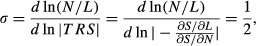

σ = d ln ( N / L ) d ln | T R S | = d ln ( N / L ) d ln | − ∂ S / ∂ L ∂ S / ∂ N | = 1 2 ,

where TRS is the technical rate of substitution (Varian 1992). An elasticity less than one indicates that, as we would expect, the two inputs are gross complements, that is, it is not possible to fully make up for lost traffic by adding extra labor. However, the assumption that this rate of substitution is constant seems problematic to us. While it might be easy to maintain a level of sales by bringing in additional traffic to replace lost labor when the staffing levels are adequate to provide the required services, increasing store traffic should not have as high of an impact when labor is already utilized to capacity. That is, the substitutability between the two inputs should be contingent on the current balance between the inputs.

To address this issue, we adopt a formulation that assumes that the output and elasticity of substitution are a function of the ratios of input factors (Karagiannis et al. 2005, Revankar 1971). Specifically, we posit that the labor‐to‐traffic ratio (ϕ = L/N) constitutes labor adequacy and drives sales generation. In other words, what matters is not labor available per se, but how labor compares to store traffic. While ϕ will normally take small values—in many store formats customers can find merchandize without the support of a sales representative—formulating the ratio as L/N makes it an increasing function of labor. Using the log‐reciprocal specification (Lilien et al. 1995) to capture the saturation effects on this ratio, the sales response function is specified as:

S = α N β e γ / ϕ = α N β e γ N / L ,

(2)

where the parameters α, β, and γ determine the store sales potential, the sales elasticity to traffic (0 < β < 1), and the response of sales to the labor adequacy (L/N) (γ < 0 when sales is an increasing function of labor). This functional form captures several relationships among store sales, store traffic, and labor supported by theoretical and empirical literature. According to queuing theory, we can reasonably expect that as the number of salespeople increases, fewer customers will leave without being served, and this will result in an increase in sales. In addition, it has been observed in retail settings that the relationship between traffic and sales is given by an increasing concave function (e.g., Perdikaki et al. 2012). Moreover, theoretical literature in service operations assumes that the relationship between revenue and labor increases at a diminishing rate (Hopp et al. 2007). This assumption has also been supported by empirical literature (e.g., Perdikaki et al. 2012) that finds that staffing levels increase sales at a diminishing rate.

The functional form is grounded on the generalized power production function that subsumes the well‐known Cobb–Douglas function and the transcendental function used by previous studies on apparel retail staffing (Kabak et al. 2008, Lam et al. 1998, Mani et al. 2015). The generalized power production function is flexible in that it does not require constant elasticity of substitution (Janvry 1972) and shows the variable elasticity of substitution that we anticipate. The elasticity of substitution of equation 2 is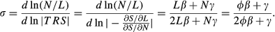

σ = d ln ( N / L ) d ln | T R S | = d ln ( N / L ) d ln | − ∂ S / ∂ L ∂ S / ∂ N | = L β + N γ 2 L β + N γ = ϕ β + γ 2 ϕ β + γ .

Since γ < 0, the elasticity of substitution of this production function is lower than the one for Lam et al.'s (1998), that is, it has an upper limit of 1/2 when the labor adequacy is high. ¹ More importantly, the elasticity of substitution is increasing in ϕ (dσ/dϕ > 0), suggesting that for the expected operating range ϕ < 1 it is more difficult to replace traffic with labor when the two inputs are out of balance. Such behaviors are expected when even more customers arrived in a situation where labor was already working at capacity.

The sales function 2 can be linearized on the inputs by taking the natural log:

ln ( S ) = ln ( α ) + β ln ( N ) + γ / ϕ .

(3)

We turn the above function into an empirically estimable fixed effects model (Wooldridge 2010) for store i at period t, in which D _i are store dummies that denote time‐invariant store characteristics such as store location and store size among others.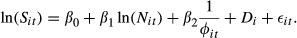

ln ( S i t ) = β 0 + β 1 ln ( N i t ) + β 2 1 ϕ i t + D i + ϵ i t .

(4)

We propose a fixed effects model, as opposed to a random effects model, as we believe that each store in our sample will be different in a unique way, not controlling for store characteristics will produce biased estimates of the coefficients.

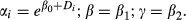
We can employ the estimated coefficients to recover structural parameters α, β, and γ. Using equations 3 and 4, we obtain the following relationships after dropping the random noise

ϵ i t

:

α i = e β 0 + D i ; β = β 1 ; γ = β 2 .

The above specification provides estimates for traffic elasticity (β) and the response to labor adequacy (γ) that takes into account all the available data (across stores and weeks), thus providing more efficient and reliable estimates for the interaction parameters. The fixed effects estimate (α _i ) accounts for the fact that stores differ in some intrinsic aspects such as location, demographics, or store size, and capture the ability to monetize the interactions between traffic and labor. Since our model includes store dummies to capture all time‐invariant aspects of a particular store, additional time‐invariant controls would be dropped from the model for being collinear to the store dummies. While a more detailed breakdown of the impact of time‐invariant effects might be desired for designing improvement strategies, the breakdown is not required for staff planning purposes. Finally, the specification in equation 4 can easily be expanded to include heterogeneity in the labor force and traffic, or to capture time variant effects by adding dummies (e.g., promotions, sales periods, etc.). Appendix A provides the specification assuming labor with two different productivity levels.

Sales Function Estimation

Using the fit sample (weeks 1–40), we adopted fixed effects modeling and include 45 dummy variables to estimate 4 (in which the base store has D _i = 0) (Cameron and Trivedi 2010). To account for AR(1) serial correlation (p < 0.001 based on a Wooldridge autocorrelation test for panel data), heteroskedasticity (p < 0.001 based on a modified Wald test for group‐wise heteroskedasticity), and cross‐sectional dependence (p < 0.001 based on three different tests for cross‐sectional independence), we adopted Driscoll and Kraay standard errors, which are robust to all three issues listed above (Hoechle 2007).

Another issue that needed to be addressed was the potential endogeneity between contemporaneous labor and sales. In a simple regression of sales and labor the coefficient of labor could be endogenously biased as (i) labor could be planned based on expected future demand, and (ii) managers could potentially observe sales and change labor accordingly. However, three separate reasons led us to believe that the endogeneity bias was mitigated in our setting. First, the fact that we use actual labor instead of planned labor should mitigate the endogeneity bias as actual labor is expected to randomly vary from planned labor due to unanticipated absenteeism. Second, controlling for traffic should also mitigate the endogeneity bias between sales and labor since actual traffic can control for unobserved events such as promotional periods when retailers would tend to schedule more labor (Perdikaki et al. 2012 have also used this approach). Finally, interviews revealed that stores plan labor based on expected traffic and that the sales associates were typically informed of their schedules a week ahead of time. As a result, the retailer does not change its staffing plans later in the week based on sales observed in the early part of the week, thus reducing the possibility of reverse causality. To verify our assumption, we ran the C‐statistic endogeneity test, which is superior to the Hausman endogeneity test as it does not require conditional homoscedasticity (Baum et al. 2003), and the Davidson‐MacKinnon test (Cameron and Trivedi 2005). We found that the null hypothesis of exogeneity is not rejected in either test (p = 0.85 and 0.65 respectively). Finally, as a robustness check, we conservatively assumed that the endogeneity bias was present and used the first and fourth lags of labor as instruments—lagged labor has been used in previous studies as a valid instrument (e.g., Perdikaki et al. 2012, Siebert and Zubanov 2010, Tan and Netessine 2014)—and found that the instrumentation makes little difference to the estimates.

Model I in Table 2 shows parameter estimates from equation 4 and their corresponding robust standard errors. Model Ia shows the estimation with the instrumental variables. We also checked the variance‐inflation‐factors (VIFs) and find no severe multicollinearity using VIF > 10 as a cutoff point (Mela and Kopalle 2002).

OPEN IN VIEWER

Table 2

Panel Data Estimates of the Sales Response Function

	Model I (FE)	Model Ia (IV)	Model II (RE)	Model III (FE)	Model IV (RE)
β0	3.656***	3.604***	1.715***	5.424***	7.202***
	(0.168)	(0.128)	(0.278)	(0.277)	(0.502)
β1 (N)	0.813***	0.831***	0.813***	0.391***	0.391***
	(0.046)	(0.038)	(0.031)	(0.058)	(0.023)
β2 (Ours) (1/ϕ)	−0.031***	−0.031***	−0.031***
	(0.003)	(0.003)	(0.002)
β2 (Lam et al.) (1/L)				−2.047***	−2.047***
				(0.336)	(0.145)
β3 ( N ¯ )			0.693***		−0.190**
			(0.091)		(0.098)
β4 (Ours) ( 1 / ϕ ¯ )			−0.072***
			(0.012)
β4 (Lam et al.) ( 1 / L ¯ )					−4.817***
					(0.664)
ρ	0.74	0.80	0.52	0.73	0.45
F statistic	108.87***	36.87***	NA	90.13***	NA
χ 2 statistic	NA	NA	696.78***	NA	647.39***
Log‐likelihood	NA	NA	854.77	NA	830.08
R 2	0.90	0.94	0.90	0.90	0.90
No. of Observations	1840	1656	1840	1840	1840

Model I shows the fixed effects estimates of our model. Model Ia treats labor as endogenous variable and shows the estimates of our model using the first and fourth lags of labor as instruments. Model II shows the Mundlak's correction estimates of our model. Models III and IV show the fixed effects and Mundlak's correction estimates of the Lam et al.'s model.

Standard errors are in parentheses. *, **, and *** denote statistical significance at the 10%, 5%, and 1% levels respectively. ρ is the share of estimated error variance accounted for by fixed effects.

The regression and all parameters are highly significant, and all estimated parameters have the expected sign and magnitude. Although simple, the proposed function is able to capture sales variation well without any additional controls. The high R ² (0.90), as well as the small root mean squared error (RMSE = 0.145), provide strong evidence that the function captures salient features of store operations and helps us build confidence in using the formulation for further analysis. Furthermore, 74% of the explained variance is due to the variance of the fixed effect estimates, suggesting that the model does an adequate job of capturing the within‐store variance over time. As a way to further assess our proposed functional form from an information theory perspective, we introduced Mundlak's correction (Mundlak 1978) that allows the use of random effects methods to estimate the model. Given a properly specified model, Mundlak's correction does not affect the parameter estimates of the fixed effect model nor the predicted outcomes. Mundlak's correction, however, permits the model to be estimated through maximum likelihood estimation (MLE) and generates robust estimates that are more efficient than fixed effect estimates (Bell and Jones 2015). Mundlak's correction incorporates store‐specific means of all time‐variant regressors as extra controls, (i.e.,

ln ( N i ) ¯

and

ϕ i − 1 ¯

), thus our sales response function becomes:

ln ( S i t ) = α i + β 1 ln ( N i t ) + β 2 1 ϕ i t + β 3 ln ( N i ) ¯ + β 4 ϕ i − 1 ¯ + ϵ i t ,

(5)

where α _i is a store‐specific intercept and assumed to be uncorrelated with other variables. Model II in Table 2 shows the parameter estimates and standard errors. Note that the estimates of β ₁ and β ₂ are identical to the FE estimates, but they are more efficient (standard errors are cut by one‐third). The estimates of the coefficients for the means of traffic and labor adequacy have the expected signs, that is, the same sign as the time‐variant effects, and are significant. As a result of these additional controls, the estimated error variance due to store fixed effects is reduced to 52%. Finally, predicted sales from Models I and II are identical—the maximum difference between predictions is within the computer rounding error, that is, 1e‐14. For prediction and analysis purposes we use Model I in the rest of the manuscript.

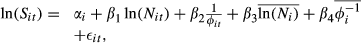
Figure 1 plots the estimated response (with 95% confidence interval) for the range covering the lower 99% of the traffic and labor adequacy values observed in our sample. The left panel shows the diminishing returns to traffic that we expect from stores being increasingly crowded (dashed line is N and is provided as reference). The right panel shows the saturation effect of labor adequacy beyond the point where the store is staffed to a level where each employee sees an average of five customers per hour (1/ϕ = 5).

OPEN IN VIEWER

Figure 1

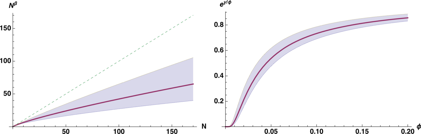
Estimated Response to Traffic and Labor Adequacy (95% CI)

Finally, the distribution of the store potentials (α _i ) under Model II has a mean of 5.620 and a standard deviation of 0.858. The distribution is fairly compact (range [3.994, 7.242]) and we found no evidence to reject that it was normally distributed (p = 0.378 Shapiro–Wilk W test). It should be noted that, having controlled for average traffic and labor adequacy, these α _i isolate all the stores’ time‐invariant factors that affect profitability. It could be possible to perform detailed analyses of the drivers of the stores’ abilities to monetize traffic and labor by treating α _i as dependent variables on regressions with hypothesized factors (e.g., store demographics, store size, competition, location). Such an analysis, however, is beyond the scope of this study.

Assessment of Sales Function

To assess the robustness of the estimated sales function, we used it to predict the realized sales in our test sample (weeks 41–52) while making smearing correction (Duan 1983) to account for errors incurred by directly exponentiating predicted ln(S _it ). Despite the fact that the test sample included significantly higher traffic periods (see discussion in subsection 6.1 and Figure 5), the function had a solid out‐of‐sample performance explaining 82.4% of the realized sales across the 46 stores and with only a 0.140 Mean Absolute Percent Error (MAPE).

To illustrate the benefits of panel estimation, we compared the performance of our estimated sales function to the store‐by‐store estimation of the Lam et al.'s (1998) formulation employed by Mani et al. (2015). In addition to the structural components in equation 1, we added time series components to account for the sales autocorrelation used by Lam et al. (1998)—see Appendix B for details. Two of the stores yielded unrealistic parameter values (β ₁ < 0 or β ₂ > 0), suggesting a specification error, and they were excluded from our comparison sample. For the remaining 44 stores, the average R ² per store was 0.70 with a standard deviation of 0.11. Considering all of the available estimates across all stores (n = 1760), the store‐by‐store estimation explained 96% of the observed sales variance (the squared correlation between actual and predicted sales). While these numbers compare well to the variance explained by our sales function (90% overall, of which 74% is explained by the store fixed effects), this marginal increase in R ² comes at a very high loss of estimation efficiency. Whereas store‐by‐store estimation with local information required 312 parameters for 44 stores, our model only required 48 parameters for 46 stores.

When using the full panel data to estimate the Lam et al.'s (1998) specification, the elasticity estimates are significant and have the expected signs and magnitudes (Model III and IV in Table 2 report the FE and Mundlak's correction estimates of the Lam et al.'s formulation). Furthermore, the model's ability to explain sales is not significantly different than that of our proposed formulation within the fit sample (weeks 1–40) (F = 0.960 and p = 0.193 for H ₀ : Difference of In‐Sample Fit = 0), nor within the test sample (weeks 41–52) (t = 0.048 and p = 0.962 for H ₀ : Difference of MSE = 0). However, assessment of the two functional forms from an information theory perspective, the established paradigm for model selection (Burnham and Anderson 2002), reveals some differences. According to Burnham and Anderson (2002), when selecting among model specifications/functional forms one should select the model with the highest information content. We use the Akaike Information Criterion (AIC)—2k − 2ln(L), where k is number of parameters in a model and ln(L) is its log likelihood—to assess the model's ability to exploit information content from the fit sample. Model II and Model IV have AICs of −1695.55 and −1646.17, respectively, indicating that model II makes better use of the information content (lower AIC) and that the relative probability of Model IV minimizing the (estimated) information loss is virtually zero (exp((AIC _II − AIC _IV )/2) (Burnham and Anderson 2002). We speculate that this difference in information content is in part reflected in the coefficient for the means for traffic (β ₃ ) having an opposite sign to the traffic elasticity (β ₁ ), suggesting that Lam et al.'s functional form is too sensitive to changes in traffic for this data set.

As discussed in the previous section, the two models differ on the assumed elasticity of substitution between production factors, that is, labor and traffic. Figure 2 plots the isoquants of the two functions as estimated using the full panel structure for the median sales ($742) in the base case store. Our formulation (solid line) shows a lower elasticity of substitution, and indicates that higher levels of staffing would be required to maintain the same levels of sales throughout the range of observed traffic. While these isoquants represent the inputs required to achieve the median sales data observed in our sample, the two functions are indistinguishable in the regions close to the medians of the fit sample. The functions, however, differ when either labor or traffic is relatively low.

OPEN IN VIEWER

Figure 2

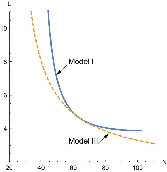
Isoquant for Median Sales on Base Case StoreNotes. Curves estimated from the parameters of Models I and III in Table 2, for a sales level of $742/week

As a final test, we estimated our model using data aggregated daily (as opposed to weekly). The model is still capable of explaining 78.6% of the daily sales variance, and does so with parameter estimates that are significant (p < 0.001) and all have the signs and magnitudes similar to the values estimated from the weekly data.

Traffic‐Based Staffing Heuristic

The estimated sales response function in subsection 4.2 provides a basis for our staffing heuristic. We treat other decisions (e.g., inventory selection, service levels, advertising) as given, and focus exclusively on labor and its impact on sales revenue by formulating an optimization problem in which labor (L _it ) is the decision variable. Consistent with prior literature (Lam et al. 1998, Mani et al. 2015), we assume that managers aim to maximize profit under constant marginal cost of labor. Even though these are common assumptions made in the literature, we acknowledge that store managers may actually take additional factors into account, yet we are not aware of the exact model they use to make their labor‐planning decisions. Our profit function is the difference of sales times the gross margin, minus the labor cost:

Max L i t π ( L i t ) = δ S i t − ω L i t = δ α i N i t β exp ( γ N i t / L i t ) − ω L i t ,

(6)

where δ is the gross margin (%) and ω is the hourly labor cost ($/hour/employee).

A closed‐form optimal solution for L _it is obtained by solving the first‐order condition of equation 6: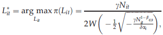

L i t ∗ = arg max L i t π ( L i t ) = γ N i t 2 W ( − 1 2 − γ N i t 1 − β ω δ α i ) ,

(7)

where W(·) is the Lambert W function—the inverse function of f(x) = xe ^x (Abramowitz and Stegun 1965) (i.e., W(x)e ^W(x) = x). While the closed‐form

L i t ∗

is valid under the constraint that the input to W(·) has to be greater than or equal to −e ⁻¹, that constraint is satisfied for our range of observed N _it and parameter estimates.

The profit function is concave in labor (L _it ), i.e.,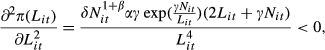

∂ 2 π ( L i t ) ∂ L i t 2 = δ N i t 1 + β α γ exp ( γ N i t L i t ) ( 2 L i t + γ N i t ) L i t 4 < 0 ,

if L _it /N _it > −γ/2, that is, if labor adequacy (ϕ _it ) meets a minimum staffing requirement of −γ/2. The minimum

N i t

in our sample is 13 customers/hour, assuming the minimum possible staffing level (

L i t = 1

) results in ϕ _it = 0.077, which is far above the estimated −γ/2 = 0.016. Thus, the profit function is concave for our operating range.

The optimal labor

L i t ∗

derived in equation 7, however, requires full information about the incoming traffic N _it for the relevant period, which managers clearly do not have at the time of the staffing decision, and thus they have to rely on traffic forecasts. To assess the effect of forecasting errors on the staffing expression above, we measure the impact of deviations of labor from the optimal staffing level as

r = π ( L i t ′ ) / π ( L i t ∗ )

, the ratio of profits from an arbitrary labor plan

L i t ′

to optimal profits. Figure 3 illustrates the impact of suboptimal staffing levels on r for fixed values of (N _it , α, γ, δ, ω) and different levels of traffic elasticity β. Figure 3 shows that the drop in profitability is more responsive to understaffing (

L i t ′ / L i t ∗ < 1

) than overstaffing (

L i t ′ / L i t ∗ > 1

). This asymmetry in the response to staffing deviations is due to the fact that while labor costs increase linearly with L _it , sales rise at a slower rate when L _it increases (i.e., decreasing returns to scale). Note also that the negative impact of understaffing is more substantial when traffic elasticity is low (β = 0.7) and store sales generation relies more on labor.

OPEN IN VIEWER

Figure 3

Impact of Suboptimal Staffing on Profit

Given that deviations in

L i t ∗

have an asymmetric impact on profitability, using traffic forecasting to identify labor requirements may result in suboptimal staffing levels as most forecasting methods rely on minimizing mean squared errors (MSE), and indirectly imply symmetric consequences of over‐ and under‐forecasting (Granger 1969). This problem is generally described in the literature as predictions with loss functions (see Lee 2008 for a review of the literature), and it has been shown that when a particular criterion (e.g., utility, monetary value) will be used to evaluate economic decisions driven by the forecasts, then it should also be used at the estimation stage of the modeling process (Gonzalez‐Rivera et al. 2007, West 1996). In our case, since we have a clear mechanism—profit function in 6—to assess the cost of a wrong forecast (the departure from optimal profits based on the suboptimal staffing level), it is justifiable (even desirable) to use readily observed data to predict optimal labor that is directly deducted from the decision criterion (Equation 6). Since sales are a function of traffic as well as the interaction between traffic and labor, the optimal staffing level is an increasing‐concave function of traffic, and, as argued in Section 3, temporal traffic variations do not contain as much variability as the variability across stores, our conjecture is that the optimal staffing should reflect past traffic flows at a store, that is,

L i t ∗ = f ( N i , t − p )

. Furthermore, if instead of using individual traffic patterns for each store we utilize traffic data across stores, we can empirically identify the structural relationships between historical traffic and optimal labor, and devise a labor plan

L ^ i t

that is near‐optimal and depends on readily observed traffic (N _i,t‐p ). This process results in an estimation that minimizes the departure from optimal profitability while explicitly considering the asymmetric response of profit to departures from optimal staffing levels, that is, the loss function.

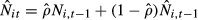
To test our conjecture that the optimal staffing level can be estimated with historical traffic, we first calculate

L i t ∗

by substituting into equation 7 the estimated parameters α, β, and γ (Model I in Table 2), the reported gross margin of the retailer for this period, δ = 0.48 (U.S. Securities and Exchange Commission 2008), and the observed N _it from the fit sample (i.e., weeks 1–40). Since we did not have access to the hourly labor cost ω for the retailer to illustrate our heuristic, we assign a value (ω = 15) based on industry statistical data from the U.S. Department of Labor and the National Retail Foundation (Bureau of Labor Statistics 2013). We later test our heuristic's sensitivity to variations in the hourly labor cost (see subsection 6.2).

Since

L i t ∗

in equation 7 is a nonlinear function of N _it , we specify a log–log model to estimate the relationship between

L i t ∗

and N _it :

ln ( L i t ∗ ( ω = 15 , δ = 0.48 ) ) = θ 0 + ∑ p θ p ln ( N i , t − p ) + d i + ϵ i t .

(8)

The idea of equation 8 is to empirically characterize optimal labor

L i t ∗

as the sum of store‐specific base levels (i.e., θ ₀ + d _i ) and a traffic‐based adjustment (i.e.,

∑ p θ p log ( N i , t − p )

) according to information up to the last p weeks. Estimating 8 enables us to identify the weights (θ _p , ∀p) assigned to past traffic to derive labor requirements. Panel data estimation is advantageous in that it uses past traffic patterns across stores (rather than local information) to generate more stable and informative estimates to develop labor requirements—a desirable attribute given the cross‐sectional dependence detected when estimating the sales response function (see subsection 4.2). Note that the FE regression in equation 8 addresses asymmetric response of profitability (see Figure 3) using the built‐in profit maximizer L* as the dependent variable/target.

Table 3 shows the fixed effects estimates and robust standard errors (in parentheses) of equation 8 (across 46 stores). We adopt the Driscoll and Kraay standard errors to account for autocorrelation, heteroskedasticity, and cross‐sectional dependence (Hoechle 2007). We consider weekly traffic lags up to four periods and find no severe collinearity as all VIFs are less than 10.

OPEN IN VIEWER

Table 3

Panel Data Estimates of Equation 8

n	θ 0	θ 1	θ 2	θ 3	θ 4	d i	R 2	Adjusted R 2	RMSE
1748	−0.545***	0.456***	0.153***	NA	NA	Included	0.937	0.935	0.108
	(0.077)	(0.056)	(0.041)
1702	−0.634***	0.423***	0.124***	0.083	NA	Included	0.937	0.935	0.108
	(0.082)	(0.062)	(0.042)	(0.055)
1656	−0.694***	0.399***	0.096**	0.072	0.079*	Included	0.939	0.937	0.107
	(0.087)	(0.063)	(0.036)	(0.047)	(0.043)
1656	0.174**	NA	NA	0.274***	0.160***	Included	0.920	0.918	0.122
	(0.088)			(0.066)	(0.058)

*p < 0.10; **p < 0.05; ***p < 0.01; The fraction of unexplained variance due to store fixed effects is 0.89.

The high (adjusted) R ² implies that past traffic is a good predictor of

L i t ∗

computed from the fit sample estimates. The diminishing weights on N _i,t−p as p increases suggest that the most recently observed traffic carries more information, which is consistent with an exponential smoothing of past traffic data. Interestingly, increasing p beyond 2 periods does not significantly improve model fit. For example, when p = 4, two extra parameters θ ₃ and θ ₄ are not significant at the 0.05 level and they only improve R ² by 0.002. Thus, we retain the simpler model with (N _i,t−1 , N _i,t−2 ). Finally, we estimate the model using (N _i,t−3 , N _i,t−4 ) to explore the possibility of generating labor plans two weeks ahead. That is, at period t−2, the manager can generate the labor plan for period t using store traffic information collected from periods t−3 and t−4. As a result, local managers would have more time to determine daily/hourly schedules and provide the detailed schedules amendable to store associates’ shift requests beforehand.

Since fixed effects modeling enables us to capture the relationships between optimal labor and past traffic in a reliable fashion, our heuristic simply capitalizes on those empirical estimates of (θ ₀ , θ _p , d _i ). Therefore, following the premise of traffic‐based (as opposed to sales‐based) labor planning, our heuristic defines weekly staffing requirements for given ω and δ as

L ^ i t ( ω , δ ) = exp ( θ 0 + ∑ p θ p ln ( N i , t − p ) + d i ) ∗ Δ ,

(9)

where Δ is the smearing correction factor (Duan 1983) to account for errors incurred by directly exponentiating ln(

L ^ i t ( ω , δ )

). The labor plan

L ^ i t ( ω , δ )

devised from equation 9 is exclusively driven by store traffic data already observed. The heuristic is realistic and easy‐to‐deploy in the sense that it only uses information that is readily available to decision makers while saving the need to extrapolate data. The above formulation exploits the structural relationships between historical traffic and optimal labor identified from the empirical estimation of 8. In the following section, we assess the proposed staffing heuristic by performing a counterfactual analysis in which we compare the performance of the heuristic against the optimal and observed staffing decisions.

Assessment of Staffing Heuristic

In this section, we assess the performance of our traffic‐based labor‐planning heuristic. By combining the two empirically verified structures (equations 4 and 8), we perform a counterfactual analysis (Kydland and Prescott 1996) to compare our heuristic's labor plans with the retailer's actual labor decisions. In addition, we assess our heuristic's sensitivity to parameter values and compare our heuristic's performance with the performance of an individual store traffic forecast‐based approach.

Heuristic Performance

Figure 4 illustrates the logic of our counterfactual analysis, in which, as in section 5, we set ω = 15 and δ = 0.48. From the fit sample (weeks 1–40) we derived estimates of (α, β, γ) in subsection 4.2 and estimates of (θ ₀ , θ _p , d _i ) in Section 5. Using those estimates and the test sample (weeks 41–52) actual traffic realizations for each store, we compute the heuristic staffing level (

L ^ i t

) from equation 9 and its corresponding profit (π(

L ^ i t

)). Similarly, we compute

L i t ∗

from equation 7 and the optimal profit

π ( L i t ∗ )

using the actual traffic realization in the test sample. For clarity of exposition, we define

h = π ( L ^ i t / π ( L i t ∗ ) )

), the ratio of profits resulting from the heuristic's staffing level to optimal profits, and

a = π ( L i t a ) / π ( L i t ∗ )

), the ratio of profits from actual staffing level to optimal profits, where

L i t a

is the observed staffing level. The two metrics (h and a) enable us to evaluate the performance of the heuristic's staffing levels and the actual staffing levels relative to the optimal staffing levels.

OPEN IN VIEWER

Figure 4

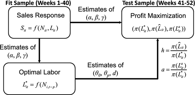
Procedure for Counterfactual Analysis

Figure 5 shows the average of h versus the average of a across 46 stores over the test sample period (weeks 41–52). In the first half of the sample (weeks 41–46), the average performance of the traffic‐based staffing heuristic is very close to optimal staffing (average performance gap (1 − h) = 0.33%). The heuristic performs better than the actual labor realization (a) by achieving significantly smaller performance gap relative to the optimal level (average performance gap (1 − a) = 3.20%, t = 12.21, p < 0.01) and lower performance variability (F = 32.45, p < 0.01). In the last 6 weeks (47–52), the heuristic's performance reveals a slight fluctuation (average performance gap (1 − h) = 2.48%) while the actual exhibits substantial performance degradation (average performance gap (1 − a) = 10.68%). Nevertheless, the heuristic still performs better than the actual in terms of a smaller gap relative to the optimal profitability (t = 13.78, p < 0.01) and lower variability (F = 14.21, p < 0.01).

OPEN IN VIEWER

Figure 5

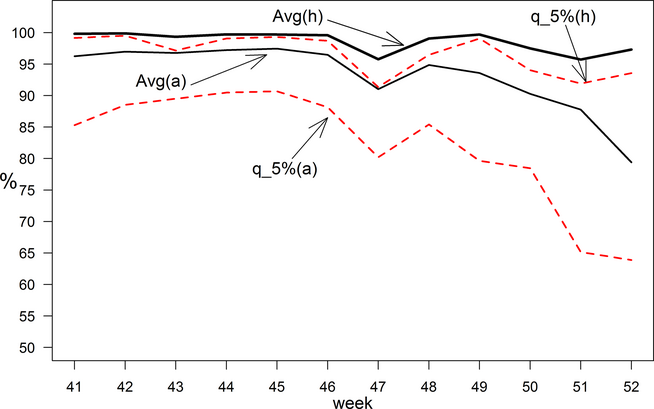
Performance of Heuristic Versus Actual and Optimal Staffing Decisions

To better understand the causes of the performance degradation of h and a during the last 6 weeks we investigate patterns of store traffic over the whole year. As shown in Figure 6, traffic flows remain stationary up to week 46 and a change occurs in the last 6 weeks. Essentially, the holiday season (Thanksgiving to Christmas) shifts the mean of traffic up and amplifies the variability of traffic among stores (not shown in the figure). Our staffing heuristic, which relies exclusively on traffic data in the past p weeks, has limited capability to address those traffic spikes. The effect is more salient because of the asymmetric response of profit to understaffing. Nonetheless, the heuristic still performs within 2.5% of the optimal profits, despite the dramatic traffic surges, for example, 50% increase in week 47 and 90% increase in weeks 51 and 52, corroborating the usefulness of exploiting structural relationships between traffic and optimal labor through across‐store fixed effects.

OPEN IN VIEWER

Figure 6

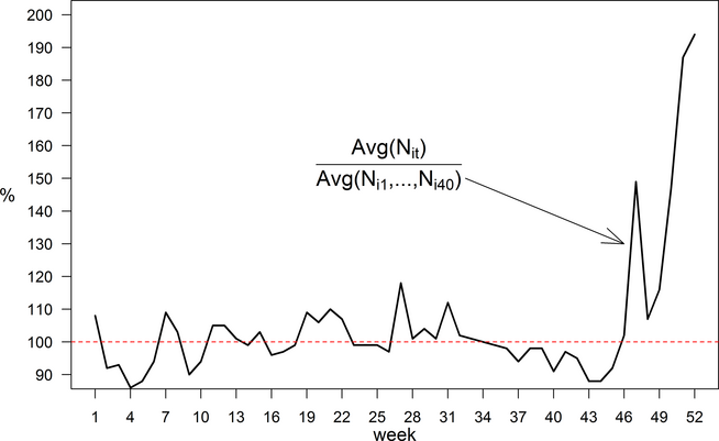
Trajectories of Store Traffic Flows over the Year

Clearly, the performance of the heuristic could be improved if we could use past years’ information to anticipate changes in traffic patterns. For instance, we could modify equation 8 into a two‐way (store and time) fixed effects model:

ln ( L i t ∗ ( ω , δ ) ) = t h e t a 0 + ∑ p θ p ln ( N i , t − p ) + d i + η P e r i o d t + ϵ i t ,

where Period _t is a set of time‐related dummy variables. These time‐related dummies could be weekly, bi‐weekly, monthly, or simply a binary indicator that separates holiday seasons from regular weeks. As such, the parameter η captures the time dynamics and the heuristic will perform even better. However, the increased cost of deploying such improvement (e.g., maintaining past year data and more complicated estimation procedures) has to be assessed against the relatively small gains available from that incremental information.

Finally, in terms of dollar values, profits from the heuristic (

π ( L ^ i t )

) are on average $27,820.69/week/store and are not statistically different from the optimal (t = −0.43; p = 0.66) (on average, the heuristic profits are just $470.00/week/store short of optimal), and significantly higher than profits from actual labor (

π ( L i t a )

) (t = 2.46; p < 0.01) (on average heuristic profits are $2,380.29/week/store higher than actual). To test the robustness of our heuristic, in the next section we conduct various analyses and focus on the first 6 weeks of the test sample under stationary traffic flows (weeks 41–46).

Heuristic Robustness

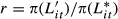
We first verify that the heuristic is robust to changes in the hourly labor cost ω by testing a wide variety of values from 10 to 25. While the precise cost information would be accessible to the retailer, we conduct the analysis as a means of assessing how the heuristic performance will change if the retailer has different compensation premiums. The left panel of Figure 7 shows the average of h versus the average of a across 46 stores and 6 weeks (weeks 41–46). The average performance of the staffing heuristic is very close to optimal staffing (average performance gap < 0.5%) regardless of the value of ω, while the performance of actual labor (a) is on average lower than the heuristic's performance (h); mainly due to some stores that were severely understaffed (see q_5%(a) line in left panel of Figure 7). In general, the traffic‐based heuristic staffs more aggressively than the retailer for ω in the realistic range of [10, 20]. The improvement of a as ω increases is because the effect of understaffing is mitigated when we assume labor is more expensive, that is, the difference between the two average staffing levels is monotonically decreasing in ω. The performance of the actual staffing practice peaks at ω = 19, but even then is still significantly inferior to h (t = 9.38, p < 0.01 H₀:(1 − h) = (1 − a)).

OPEN IN VIEWER

Figure 7

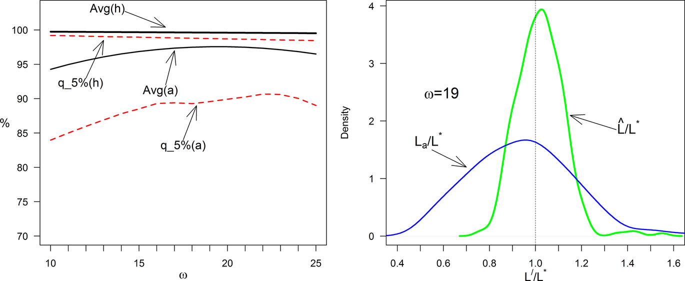
Impact of Wage on Heuristic Performance

Note that one of the advantages of the heuristic is the reduced variability of performance across stores as the full panel information is being used to estimate the sales response and predict the optimal labor. To better articulate this point, we compare heuristic‐generated labor and actually realized labor to optimal labor. The right panel of Figure 7 illustrates estimated probability densities of

L ^ / L ∗

and L _a /

L ∗

at ω = 19 (where L _a reaches its highest profitability). Several observations can be made from the figure. First, our heuristic exhibits much lower variability and in most cases its deviation from

L ∗

is within ± 20%. As illustrated in Figure 3, such modest departures from the optimal staffing level have limited impact on profitability, explaining the low variability of h in the left panel of Figure 7. Second, the slight right skewness of

L ^ / L ∗

is an indicator of the asymmetric response of profitability to overstaffing and understaffing. Since overstaffing is preferred for the profit function, our heuristic, that considers the effects of prediction loss, has a bias toward the overstaffing side. Third, in addition to exhibiting higher performance variability, the distribution of L _a /

L ∗

is skewed to the left and reflects that there are more instances of under‐staffing (L _a /

L ∗

< 1) and with a larger deviation from

L ∗

.

We further evaluate the performance of generating labor plans two weeks ahead, as doing so would allow store managers to have more time making local adjustments of labor schedules. Specifically, we apply the estimated θ ₃ and θ ₄ (Table 3) to lagged traffic data (N _i,t−3 , N _i,t−4 ) and compute staffing levels from equation 9. Table 4 shows the performance comparison under different values of ω. The heuristic with either (N _i,t−1 , N _i,t−2 ) or (N _i,t−3 ,N _i,t−4 ) performs significantly better than actual labor decisions. Also, the staffing heuristic achieves much lower performance variability across stores and weeks. For instance, for the case where ω = 15, the performance of the labor plan fixed two weeks in advance (N _i,t−3 ,N _i,t‐4 ) drops only 0.19% from the plan made for the current period, with a minimal increase in variability relative to the (N _i,t−1 , N _i,t−2 ) case of 0.27%—that is, 0.93–0.66.

OPEN IN VIEWER

Table 4

Performance Comparison among Different Staffing Approaches

	Actual labor (a)	Traffic lag 1–2(h)	Traffic lag 3–4(h)	Exponential smooth (h e )	ARIMA (2, 1)(h a )
ω = 10
Mean (%)	94.17	99.75	99.61	99.70	99.68
t‐test		18.51*	17.93*	18.46*	18.39*
SD (%)	4.95	0.49	0.71	0.57	0.59
F‐test		95.18*	47.84*	76.50*	70.15*
ω = 15
Mean (%)	96.80	99.67	99.48	99.61	99.58
t‐test		12. 21*	11.22*	12.00*	11.87*
SD (%)	3.82	0.66	0.93	0.74	0.78
F‐test		32.45*	16.22*	26.32*	24.20*
ω = 20
Mean (%)	97.53	99.60	99.37	99.52	99.49
t‐test		8.94*	7.73*	8.60*	8.45*
SD (%)	3.72	0.82	1.16	0.92	0.96
F‐test		20.61*	10.23*	16.40*	15.10*

The analysis (n = 46 * 6 = 276) is across 46 stores and 6 weeks. t‐test H ₀ : Mean a‐Mean h = 0. F‐test H ₀ : Variance a/Variance h = 1.

^† p < 0.05, *p < 0.01.

As mentioned in Section 5, the heuristic relies on estimates from the whole panel data set without extrapolating traffic data. As a final benchmark, we test two extrapolative traffic forecasting approaches. The first approach is exponential smoothing and is selected for comparison because of its recognized performance and popularity in practice (Achabal et al. 2000). We estimate the optimal exponential smoothing coefficient ρ _i for each store using the fit sample and the starting condition

N ^ i t = N i t

We generate a traffic forecast

N ^ i t = ρ ^ N i , t − 1 + ( 1 − ρ ^ ) N ^ i , t − 1

and substitute

N ^ i t

into equation 7 to devise labor plans (

L ^ i t ∗

) for the test sample period. The optimal exponential smoothing achieves a RMSE of 7.57 and a MAPE of 0.09 over the sample. The second approach is an autoregressive integrated moving average (ARIMA) model (Washington et al. 2011) adopted by Lam et al. (1998). We apply ARIMA (p = 2, q = 1) (see Appendix C for model selection details) to generate traffic forecast

N ^ i t

that is also inserted into equation 7 to compute

L ^ i t ∗

. The ARIMA (2, 1) model achieves a RMSE of 6.74 and a MAPE of 0.07 over the sample. The last two columns of Table 4 show that the two staffing approaches based on local exponential smoothing (h ^e = π(

L ^ i t ∗

)/π(

L i t ∗

)) and ARIMA (h ^a = π(

L ^ i t ∗

)/π(

L i t ∗

)) outperform actual labor staffing decisions. However, our proposed heuristic using the whole panel to derive global weights on (N _i,t‐1 , N _i,t‐2 ) achieves a significantly smaller performance gap relative to the optimal (t‐test) and significantly lower variability (F‐test) across the whole range of ω when compared to the local exponential smoothing h ^e (t = 2.62, p < 0.01; F = 1.19, p < 0.01) and ARIMA h ^a (t = 4.76, p < 0.01; F = 1.37, p < 0.01) approaches. Upon inspection, it is evident that the extrapolative forecast methods perform well because their predictions are within 10% of the realized value (i.e., MAPE < 0.10, and the profit function is quite insensitive to small forecasting errors (see Figure 3)). That said, the statistically significant difference between our heuristic and the extrapolative methods comes from the more stable estimates of desired labor that emerge from the panel estimation. This finding suggests that the value of the heuristic emerges more from setting the appropriate target level (

L i t ∗

) based on the sales response function rather than from a precise traffic forecast.

Discussion

Our study takes a grounded approach to develop a retail labor‐planning framework, which avoids the pitfall of allocating labor capacity solely based on a rudimentary calculation of expected sales without fully utilizing knowledge about customer traffic. Our study has several distinct features. First, when formulating the sales response function we introduced the notion of labor adequacy. Our focus on labor adequacy aims to enhance service quality and conformance quality in actual store operations, since adequate/abundant labor capacity is instrumental in reducing work pressure and speeding up customer service (Oliva and Sterman 2001); ensuring correct execution of in‐store logistic tasks (Ton 2014); and maintaining inventory information accuracy (Chuang and Oliva 2015). Second, our proposed sales function exhibits variable elasticity of substitution between traffic and labor, which is expected in a retail setting, and is more capable of explaining sales performance under extreme conditions of input factors. The variable elasticity of substitution between labor and traffic, together with the labor adequacy, shed light on the importance of balancing labor‐to‐traffic ratios in practice. Third, in order to exploit information available across stores, we adopted panel estimation methods for our sales function as well as the staffing rule. Doing so helps us not only isolate time‐invariant store differences that affect the stores’ ability to turn traffic into sales, but also develop labor requirements that are commensurate to other stores’ staffing levels as opposed to levels that are continuation trends of a store's current practices. As a result of the robust and efficient panel estimation, our heuristic performs fairly well under both stable and extreme traffic conditions. Last, our study goes beyond establishing static correlations between variables and contributes to the growing body of empirical research on the effects of labor on retail performance (Fisher et al. 2006, Mani et al. 2015, Netessine et al. 2010, Perdikaki et al. 2012, Ton 2009, Ton and Huckman 2008). Researchers who aim to develop data‐driven and easy‐to‐use staffing rules can refer to our modeling framework and extend our idea to other labor‐intensive service settings such as restaurants, banks, and hospitals. Moreover, researchers who intend to empirically assess retail labor productivity should find the proposed sales response function applicable given the function properties.

Several limitations of our study pinpoint opportunities for future research. First, our analysis assesses a single apparel retail chain, which allows us to implicitly control unobservable firm‐level factors such as pricing policies, manager incentive schemes, and types of merchandise. Analyzing stores of the same firm contributes to a deep understanding of the context but somewhat limits the generalizability of our results. Subsequent studies should attempt to further explore the effects of labor and traffic on performance in other service settings. Second, we adopt a fixed effects estimation to control for several unobservable time‐invariant store‐level factors that could affect sales. We acknowledge that several other factors such as labor experience, employee turnover, and inventory levels, for which we do not possess data, could drive store sales performance. Third, we take an aggregate view on planning labor capacity and derive weekly labor requirements. While the detailed daily/hourly workforce scheduling is not explicitly addressed in our study, we have shown that the proposed sales response function works with that granularity. Lastly, given that we only have data on total labor hours, we cannot differentiate full‐time labor from part‐time labor, which could differ in experiences, attitudes, and productivity. For example, Chuang and Oliva (2015) find that the mix of full‐time and part‐time labor has significant impact on inventory data quality. In Appendix A, we show how our sales response function can be modified to distinguish between full‐time and part‐time labor. Future research may incorporate labor mix into a modeling framework, empirically identify its effect, and develop more comprehensive staffing rules.

Despite these limitations, our modeling efforts carry pragmatic implications for retail practitioners. First, our study proposes a methodology that guides retailers to utilize aggregate information to determine labor requirements. Since many retailers have recently invested in traffic counting technology and have started using such technology to support labor planning, retailers who possess traffic count data could adopt our framework to derive weekly labor hour requirements at their stores. These weekly requirements could then be used by store managers as guidance to identify the mix of labor and perform daily as well as hourly level scheduling. Second, the proposed heuristic is easy to implement in that it merely requires readily available data and does not rely on sophisticated forecasting mechanisms. Our heuristic applies fixed effects estimation to derive weights on past traffic and outperforms an extrapolative approach that requires store‐level traffic forecasting. The weights on observed traffic information can be estimated and updated in a spreadsheet. Third, unlike many existing retail labor management systems that focus on minimizing labor costs and often result in understaffing, our labor‐planning framework provides an alternative to match labor with traffic so as to achieve better sales performance. By aiming for reduction of labor‐traffic‐mismatches, we expect our heuristic's recommended staffing levels not only to positively affect service delivery but also to relieve employee work pressure/fatigue to a certain extent. Last, retailers can take advantage of the robustness of our heuristic to lagged traffic information to develop aggregate labor plans that become input to daily/hourly schedules and apprise their employees of their schedules several weeks in advance. Such an approach can allow retailers to accommodate employees shift requests/preferences without sacrificing profitability. This idea of being accommodative to store labor is actually found to be beneficial for store execution and profits in high‐performance retail companies (Ton 2014).

Footnotes

Estimation Equation for Heterogeneous Labor Productivity

Estimating Lam et al.'s ( 1998 ) Sales Response Function

Traffic Forecasting of Lam et al. ( 1998 )

Acknowledgments

The authors are grateful for the helpful suggestions provided by Nicole DeHoratius, the Senior Editor, and two referees. The authors also thank Gregory Heim, James Abbey, and Ram Janakiraman for their comments and suggestions, which helped improve the content and presentation of the manuscript.

1

The constraint σ > 0 also reduces the viable range for the response to labor adequacy to −βϕ< γ < 0.

References

1.

Abramowitz M. Stegun I. A. . 1965. Handbook of Mathematical Functions: With Formulas, Graphs, and Mathematical Tables. Dover Publications, New York, NY.

Go to Reference

2.

Achabal D. D. Mclntyre S. H. Smith S. A. Kalyanam K. . 2000. A decision support system for vendor‐managed inventory. J. Retail. 76(4): 430–454.

Go to Reference

3.

Baker Retail Initiative . 2007. Shoppers at Risk: An Annual Study of Retail Dissatisfaction. Executive Summary. The Wharton School, University of Pennsylvania, Philadelphia.

Go to Reference

4.

Baltagi B. H. 2001. Econometric Analysis of Panel Data, 2nd edn. John Wiley & Sons Ltd, Chichester, UK.

Go to Reference

5.

Baum C. F. Schaffer M. E. Stillman S. . 2003. Instrumental variables and GMM: Estimation and testing. STATA J. 3(1): 1–31.

Go to Reference

6.

Bell A. Jones K. . 2015. Explaining fixed effects: Random effects modeling of time‐series cross‐sectional and panel data. Politi. Sci. Res. Methods 3(1): 133–153.

+ Show References

7.

Box G. E. Jenkins G. M. Reinsel G. C. . 2008. Time Series Analysis: Forecasting and Control. Wiley, New Jersey, NJ.

Go to Reference

8.

Bureau of Labor Statistics . 2013. Pay & Benefits. http://www.bls.gov/data/#wages (accessed date May 14, 2015).

Go to Reference

9.

Burnham K. P. Anderson D. R. . 2002. Model Selection and Multi‐Model Inference: A Practical Information‐Theoretic Approach, 2nd edn. Springer, New York, NY.

+ Show References

10.

Cameron A. C. Trivedi P. K. . 2005. Microeconometrics: Methods and Application. Cambridge University Press, Cambridge, UK.

+ Show References

11.

Cameron A. C. Trivedi P. K. . 2010. Microeconometrics Using STATA, 2nd edn. Stata Press, College Station, TX.

Go to Reference

12.

Cascio W. 2006. Decency means more than ‘always low prices: A comparison of Costco to Wal‐Mart's Sam's Club. Acad. Manag. Perspect. 20(3): 26–37.

Go to Reference

13.

Chuang H. H. Oliva R. . 2015. Inventory Record Inaccuracy: Causes and Labor Effects. J. Oper. Manage. 39–40: 63–78.

+ Show References

14.

DeHoratius N. Raman A. . 2008. Inventory record inaccuracy: An empirical analysis. Manage. Sci. 54(4): 627–641.

Go to Reference

15.

Duan N. 1983. Smearing estimate: A nonparametric retransformation method. J. Am. Statisti. Assoc. 78(383): 605–610.

+ Show References

16.

Fisher M. L . 2004. To me it's a store. To you it's a factory. ECR J. 4(2): 9–18.

Go to Reference

17.

Fisher M. L. Krishnan J. Netessine S. . 2006. Retail store execution: An empirical study. Working paper, The Wharton School, University of Pennsylvania, Philadelphia.

+ Show References

18.

Gonzalez‐Rivera G. Lee T. Yoldas E. . 2007. Optimality of the RiskMetrics VaR model. Fin. Res. Lett. 4(3): 137–145.

Go to Reference

19.

Granger C. W. J. 1969. Prediction with a generalized cost of error function. OR 20(2): 199–207.

+ Show References

20.

Griliches Z. Hausman J. A. . 1986. Errors in variables in panel data. J. Econometr. 31(1): 93–118.

+ Show References

21.

Hoechle D. 2007. Robust standard errors for panel regressions with cross‐sectional dependence. STATA J. 7(3): 281–312.

+ Show References

22.

Hopp W. J. Iravani S. M. R. Yuen G. Y. . 2007. Operations systems with discretionary task completion. Manage. Sci. 53(1): 61–77.

Go to Reference

23.

Hsiao C. 2003. Analysis of Panel Data. Cambridge University Press, Cambridge, UK.

Go to Reference

24.

Janvry A. D. 1972. The generalized power production function. Am. J. Agric. Econ. 54(2): 234–237.

Go to Reference

25.

Kabak O. Ulengin F. Aktas E. Onsel S. Topcu Y. I. . 2008. Efficient shift scheduling in the retail sector through two‐stage optimization. Eur. J. Oper. Res. 184(1): 76–90.

+ Show References

26.

Karagiannis G. Palivos T. Papageorgiou C. . 2005. Variable elasticity of substitution and economic growth: Theory and evidence. Diebolt C. Kyrtsou C. , eds. New Trends in Macroeconomics. Springer, Berlin, Germany, 21–37.

Go to Reference

27.

King G. 1998. Unifying Political Methodology: The Likelihood Theory of Statistical Inference. Cambridge University Press, Cambridge, UK.

Go to Reference

28.

Klevmarken N. A. 1989. Panel studies: What can we learn from them? Introduction Eur. Econ. Rev. 33(2): 523–529.

Go to Reference

29.

Kydland F. E. Prescott E. C. . 1996. The computational experiment: An econometric tool. J. Econ. Perspect. 10(1): 69–85.

+ Show References

30.

Lam S. Vandenbosch M. Pearce M. . 1998. Retail sales force scheduling based on store traffic forecasting. J. Retail. 74(1): 61–88.

+ Show References

31.

Lee T . 2008. Loss functions in time series forecasting. Darity W. A. , ed. International encyclopedia of the social sciences, Vol. 9, 2nd edn. Macmillan Thomson Gale Publishers, Detroit, 495–502.

Go to Reference

32.

Lilien G. L. Kotler P. Moorthy K. S. . 1995. Marketing Models. Prentice‐Hall Inc, Englewood Cliffs, New Jersey.

+ Show References

33.

Mani V. Kesavan S. Swaminathan J. M. . 2015. Estimating the impact of understaffing on sales and profitability in retail stores. Prod. Oper. Manag. 24(2): 201–218.

+ Show References

34.

Mela C. F. Kopalle P. K. . 2002. The impact of collinearity on regression analysis: The asymmetric effect of negative and positive correlations. Appl. Econ. 34(6): 667–677.

Go to Reference

35.

Mundlak Y. 1978. Pooling of time‐series and cross‐section data. Econometrica 46(1): 69–85.

+ Show References

36.

Netessine S. Fisher M. L. Krishnan J. . 2010. Labor planning, execution, and retail store performance: An exploratory investigation. Working paper, The Wharton School, University of Pennsylvania, Philadelphia.

+ Show References

37.

Oliva R. Sterman J. D. . 2001. Cutting corners and working overtime: Quality erosion in the service industry. Manage. Sci. 47(7): 894–914.

+ Show References

38.

Oliva R. Sterman J. D. . 2010. Death spirals and virtuous cycles: Human resource dynamics in knowledge‐based services. Maglio P. P. Kieliszewski C. A. Spohrer J. C. , eds. Handbook of Service Science. Springer, New York, 321–358.

Go to Reference

39.

Pastor R. Olivella J. . 2008. Selecting and adapting weekly work schedules with working time accounts: A case of a retail clothing chain. Eur. J. Oper. Res. 184(1): 1–12.

Go to Reference

40.

Perdikaki O. Kesavan S. Swaminathan J. M. . 2012. Effect of traffic on sales and conversion rates of retail stores. Manuf. Serv. Oper. Manag. 14(1): 145–162.

+ Show References

41.

Raman A. DeHoratius N. Ton Z. . 2001. Execution: The missing link in retail operations. Ca. Manag. Rev. 43(3): 136–152.

Go to Reference

42.

Revankar N. S. 1971. A class of variable elasticity of substitution production functions. Econometrica 39(1): 61–71.

Go to Reference

43.

Siebert W. S. Zubanov N. . 2010. Management economics in a large retail company. Manage. Sci. 56(8): 1398–1414.

+ Show References

44.

Tan T. F. Netessine S. . 2014. When does the devil make work? An empirical study of the impact of workload on worker productivity. Manage. Sci. 60(6): 1574–1593.

Go to Reference

45.

Ton Z . 2009. The effect of labor on profitability: The role of quality. Working paper, Harvard Business School, Harvard University, Boston.

+ Show References

46.

Ton Z. 2014. The Good Jobs Strategy: How the Smartest Companies Invest in Employees to Lower Costs and Boost Profits? New Harvest, New York, NY.

+ Show References

47.

Ton Z. Huckman R. S. . 2008. Managing the impact of employee turnover on performance: The role of process conformance. Organ. Sci. 19(1): 56–68.

+ Show References

48.

Ton Z. Raman A. . 2010. The effect of product variety and inventory level on retail store sales: A longitudinal study. Prod. Oper. Manag. 19(5): 546–560.

Go to Reference

49.

U.S. Securities and Exchange Commission . 2008. http://secdatabase.com/ (accessed date May 14, 2015).

Go to Reference

50.

Varian H. R. 1992. Microeconomic Analysis, 3rd edn. W. W. Norton & Company Inc, New York.

Go to Reference

51.

Washington S. P. Karlaftis M. G. Mannering F. L. . 2011. Statistical and Econometric Methods for Transportation Data Analysis. CRC Press, Boca Raton, FL.

+ Show References

52.

West K. 1996. Asymptotic inference about prediction ability. Econometrica 64(5): 1067–1084.

+ Show References

53.

Wooldridge J. M. 2010. Econometric Analysis of Cross Section and Panel Data, 2nd edn. The MIT Press, Boston.

+ Show References