Pricing Strategies under Behavioral Observational Learning in Social Networks

Abstract

The increasing pervasiveness of social networks allows users to share purchase behaviors with their online friends. In this study, we examine optimal pricing strategies of a monopolistic firm using an analytical model that accounts for behavioral observational learning in social networks. We show that a seller could potentially control the information available to future customers and induce behavioral observational learning, using an information‐revealing pricing strategy. This result suggests that offering introductory discounts is not always an effective method to boost purchases in social networks. It could prevent the behavioral observational learning that would increase future customers' willingness to pay.

Keywords

observational learning social networks optimal pricing pricing strategy

Introduction

And therein lay the secret to all fads: the herd instinct. People wanted to look like everybody else. That was why they bought white bucks and pedal pushers and bikinis. Willis, C. (1996) p. 33

The rapid growth of social networks has been changing the way consumers interact with businesses. In the canonical models of observational learning (Banerjee 1992, Bikhchandani et al. 1992), people make their decisions on whether to dine on the basis of how many consumers are already in a restaurant. The essence of observational learning is that an individual's decision is affected by the observation of others' choices because of its informational content. Social networking sites are making people's behaviors more observable to their friends. Socially shared purchases have become a mainstream activity of consumers and one of the top drivers for online sales. For example, Amazon encourages consumers to socially share their purchases across Facebook, Twitter, and e‐mail. Recently, the increasing pervasiveness of location‐acquisition technologies has allowed users to “check in” at physical venues and share the locations with their online friends. Consumers can use location‐based services (e.g., Foursquare, Facebook Place, or Google+) to navigate and engage with venues by receiving relevant coupons or ads based upon the location. Introducing socially shared purchases is a relatively new feature of e‐commerce that can drive both significant referral visits and conversion uplift. The use of social sharing content to show friend purchase activity leads to significant observational learning on Facebook and other social networking websites.

The widespread adoption of social networks adds an important dimension to prior observational learning literature. As a result of the new marketing technology of social networks, a striking difference has arisen: In the previous observational learning story (e.g., Banerjee 1992), people can observe all of the choices made by people before them, including many anonymous consumers. This is not an appropriate assumption in social networks. In the current practice, people are connected by a social network, and they observe only their friends' choices. Acemoglu et al. (2011) explored an observational learning model over a general social network. However, a seller's pricing strategies are absent from the model. On the other hand, a large stream of literature has been devoted to investigating sellers' pricing strategies in the absence of observational learning. Kumar and Sethi (2009) examined an optimal control model of dynamic pricing for web content providers. Gupta et al. (2011) studied investment incentives for network infrastructure owners under different pricing strategies. August and Niculescu (2013) examined how a software firm optimally determines its pricing in a setting where it can harness customer error reporting. Sellers' other strategies, such as the introduction of product upgrades (Ji et al. 2011, Mehra et al. 2014) and introduction of agency model for digital goods (Tan and Carrillo 2017, Tan et al. 2016), have also been considered in the literature.

In this study, we extend the literature by examining the interaction of pricing strategies and observational learning in social networks. We propose a behavioral inference rule that is cognitively simple for a consumer's complex decision making in social networks and relax a key assumption that has been implicitly accepted in prior observational learning literature: A consumer can observe the choices of all others who have made their choices ahead of her.

When designing its optimal pricing policy, a monopolistic firm could potentially control the process of observational learning using different pricing strategies. In our context, a firm faces the following two trade‐offs of using different pricing strategies: (i) In standard static monopoly pricing, a monopolistic firm faces a downward sloping demand curve. Setting a higher price implies a higher revenue per unit (positives associated with an increase in price), but on the other hand, the quantity demanded decreases with the price (negatives associated with an increase in price). This is the conventional static trade‐off discussed in the pricing literature. (ii) In our study, we focus on the second tradeoff associated with positives and negatives of pricing strategies in a dynamic setting. If the price is too high, then very few early consumers will adopt the product, and the monopolistic firm will not be able to use observational learning to boost its sales in the second period. On the other hand, if the price is too low, the effect of observational learning is also limited because late consumers would know that their friends purchased the product due to the low price instead of its high quality.

Therefore, if the price is set sufficiently high (information revealing) so that prior friends receiving different private signals make different purchase decisions, a subsequent consumer is able to infer the product quality through the decisions of her friends. Conditional on an information‐revealing pricing strategy, the subsequent consumer is more likely to infer that the product quality is high when the number of her friends who adopt the product is larger (Lemma 2 in section 4.3). If the firm charges such a low price (information pooling) in the first period that almost all consumers adopt the product, this price would not reveal any quality information of the product to future consumers. In this case, observational learning will play no role in increasing the future consumers' willingness to pay.

In this study, we develop a two‐period model and compare the optimal pricing policy under rational observational learning with that under behavioral observational learning. An important feature of our model is that the intensity of observational learning is endogenously determined by different pricing strategies. We find that the information‐revealing pricing strategy is optimal only in extreme market conditions (i.e., the ex ante uncertainty of product quality is very high or consumers have very precise private information on product quality) under rational learning. However, under behavioral learning, the use of information‐revealing pricing strategy is optimal in a wide range of market conditions. This result differs from that in the seeding literature (e.g., Dou et al. 2013, Ho et al. 2012). Introductory discounts could prevent observational learning, and hence are not always an effective method to boost purchases.

Literature Review

There are two fundamental supporting pillars in our research: (i) optimal pricing of experience goods, and (ii) social learning. Therefore, our study is closely related to these two streams of literature.

The Literature on Optimal Pricing of Experience Goods

A central topic of our study is the optimal pricing strategies. In a seminal paper, Shapiro (1983) examined a monopolist's optimal pricing strategies for non‐durable experience goods. Villas‐Boas (2006) extended the model to a duopoly setting with dynamic competition. Dudine et al. (2006) investigated dynamic monopoly pricing of storable goods in an environment where demand changes over time. In a continuous‐time model, Bergemann and Valimaki (2006) analyzed the optimal price path for a monopolist that sells an experience good over time to a population of heterogeneous buyers with independent private valuations. They found that the optimal price trajectory critically depends on whether the market is a niche or mass market. Jing (2011a) explored the effectiveness of two common pricing strategies—behavior‐based price discrimination and price commitment in a two‐period model of non‐durable experience goods. Jing (2011b,c) examined the impact of social learning on dynamic pricing of durable goods in a two‐period model. Fainmesser and Galeotti (2016) developed a model in which a monopoly sells a network good and price discriminates based on information about consumers' influence and consumers' susceptibility to influence.

The focus of our study is also the optimal pricing strategy of a monopolistic firm. However, our study differs from this stream of literature in two aspects. First, the prior literature has largely focused on consumer self‐learning through consumption in a setting of non‐durable goods, where the product is repeatedly purchased and learning occurs during consumption (e.g., Bergemann and Valimaki 2006, Jing 2011a, Shapiro 1983, Villas‐Boas 2006). In contrast, we focus on consumers' observational learning from friends' decisions. It is worth noting that Jing (2011b,c) and Fainmesser and Galeotti (2016) also considered the impact of other consumers' purchase decisions. However, our underlying learning mechanism is quite different from theirs. In Jing (2011b,c), the underlying learning mechanism behind consumer interaction is not modeled explicitly, and the speed of consumer social learning is controlled by an exogenous parameter of learning intensity. The underlying mechanism in Fainmesser and Galeotti (2016) is network effects (payoff externalities): A consumer's payoff depends positively on the number of other people who consume the product. In contrast, our learning mechanism is explicitly modeled in the framework of observational learning (based on information externalities¹ ): Consumers infer product quality through their friends' decisions. More importantly, the intensity of observational learning in our model is endogenously controlled by the firm's pricing strategies (information‐pooling strategy vs. information‐revealing strategy).

Second, our paper studies the interaction between observational learning and optimal pricing in a unique social network context, which has been overlooked in the previous optimal pricing literature. We propose a behavioral inference rule that is cognitively simple for consumers' complex decision making in social networks, and demonstrate that the optimal pricing strategy under behavioral observational learning is different from that under conventional rational observational learning.

The Literature on Social Learning and Diffusion

In the prior literature, there are two important forms of social learning: word‐of‐mouth communication (Chevalier and Mayzlin 2006, Samiei and Tripathi 2014) and observational learning (Banerjee 1992). In general, consumers' purchase decisions can be influenced by friends' opinions (word of mouth), and/or friends' purchase behaviors (observational learning). Chen et al. (2011) differentiated between word of mouth and observational learning using a natural experiment on Amazon. In our study, we focus on the second underlying mechanism: consumers' knowledge of the product is only through observing the actions of their friends, that is, observational learning.

A handful of empirical studies have explored observational learning in different contexts. Duan et al. (2009) empirically examined herd behavior and informational cascades in the context of online software adoption. Zhang and Liu (2012) studied observational learning in microloan markets. Qiu et al. (2014a) estimated a structural model of restaurant discovery and observational learning using data from a major location‐based social networking website in China. Our present work differs from these prior studies in two aspects. First, most of the previous studies focused exclusively on the consumer side and examine whether and how a consumer is influenced by observational learning. In this study, we explore how a monopolistic seller can induce observational learning, using pricing strategies to maximize its profit. Second, we relax the assumption of rational observational learning, in which a consumer can observe all prior consumers' decisions, and propose a more realistic behavioral inference rule in a context of social networks. We also compare the optimal pricing policy under our behavioral inference rule with that under rational learning. Our analytic model provides a framework for further empirical work on observational learning and optimal pricing in social networks.

In the full‐rationality theory of observational learning (Banerjee 1992, Bikhchandani et al. 1992), besides realizing that the previous movers' actions reflect these movers' own signals, each consumer also takes into account that these predecessors themselves also infer from still earlier actions. Such a high rationality requirement seems unrealistic or extreme in certain circumstances (Eyster and Rabin 2010), especially when a consumer does not have complete information on the structure of social networks. An extensive literature shows that people have limited cognitive abilities to process information and provides evidence that consumers use decision rules that are cognitively simple (Kahneman 2003, Lacetera et al. 2012). The question of how decision‐makers' cognitive constraints limit their ability to process available information has received increasing interest in the behavioral operations management literature (Bendoly et al. 2010). Recently, behavioral issues in supply chain pricing have also been discussed (Katok et al. 2014).

It is also instructive to contrast our model with the literature on diffusion (Jiang and Jain 2012). Ho et al. (2012) further extended the two‐segment diffusion model and examine the role of introductory discounts in boosting product purchases. In this study, we do not assume that social contagion is at work in every instance and try to open the black box of the diffusion mechanism. A consumer makes an inference about product quality by observing other people's choices. The adoption behaviors of her friends are informative signals that reflect the product quality, but do not directly enter her utility function.

Comparison of Different Learning Mechanisms

A Motivating Example

We begin our analysis by describing an illustrative example to show the difference between behavioral observation learning and rational observational learning. In Appendix S3, we conduct a laboratory experiment and empirically show the use of observational learning mechanism in reality. A basic (implicit) assumption of our study is that consumers use observational learning to make their purchase decisions. Although it is a common assumption in the prior observational learning literature, in social network settings, it is not clear whether consumers will actually use observational learning in their process of decision making. In other words, a consumer can simply talk to his/her friends who have adopted the product and ask them if they found the quality to be high or low. This is particularly plausible in the context of social networks. Therefore, in our experiment, we want to investigate under which conditions consumers are more likely to employ the observational learning mechanism instead of asking their friends directly.

More specifically, in our experiment, we are interested in two factors: (i) the price of a product, and (ii) the strength of social ties between consumers. Our experimental results showed that consumers are more likely to employ the observational learning mechanism instead of talking to their friends directly when the price is lower (the benefit of asking friends' opinions is smaller) and when the strength of social tie is weaker (the cost of asking friends/acquaintances' opinions is higher). In reality, the observational learning mechanism is more likely to be used when your ordinary Facebook friends (your acquaintances) share their purchases of small ticket items. In particular, Gee et al. (2016) found that weak ties (acquaintances) comprise a majority of a person's social network, so the use of the observational learning mechanism is likely to be common in practice.

In our motivating example, we consider consumers decide whether to buy a tablet accessory, such as a case with keyborad or an iPad mount. We choose this specific product category because our analytical model focuses more on the vertical quality dimension in which consumers share very similar opinions than the horizontal differentiation (tastes).² Moreover, in our laboratory experiment (see Appendix S3), we find that consumers are more likely to employ observational learning mechanism when the product is a small ticket item, such as tablet accessory.

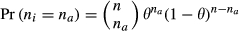
The quality of the product is unknown to all consumers and is represented by a binary random variable: V ∈ {V _H, V _L}, and V _H > V _L > 0. We assume a common prior on the probability that the product is of high quality:

\Pr (V_{H}) = 1 / 2

. The utility function is assumed to be linear in product quality: A consumer obtains a utility level of V _H from a high quality product, and a utility level of V _L from a low quality product. We also assume that the price of the product is

\frac{1}{2} V_{H} + \frac{1}{2} V_{L}

. We will consider the pricing problem later in the formal model. In this example, actually we can choose any price that satisfies

\frac{1}{4} V_{H} + \frac{3}{4} V_{L} < p \leq \frac{3}{4} V_{H} + \frac{1}{4} V_{L},

but for the convenience of the calculation, we use

p = \frac{1}{2} V_{H} + \frac{1}{2} V_{L}

. On the other hand, we have assumed that the common prior on product quality

\Pr (V_{H}) = 1 / 2

. Therefore, it is reasonable to set the price to be

p = \frac{1}{2} V_{H} + \frac{1}{2} V_{L}

There are 100 consumers in this town, and they are connected by a social network. Using the social network service, consumers can see if any of their friends have recently bought the product. Consumers make sequential decisions: 50 consumers decide whether to buy the product in week 1, 50 consumers decide whether to buy the product in week 2. Before a consumer makes her decision, she receives a binary private signal independently and identically drawn from a Bernoulli distribution. The signal can be either S _H or S _L, and without loss of generality, we further assume that the signals are informative with the following values:

\Pr (S_{H} | V_{H}) = \Pr (S_{L} | V_{L}) = \frac{3}{4}

, and

\Pr (S_{L} | V_{H}) = \Pr (S_{H} | V_{L}) = \frac{1}{4}

We focus on a simple social network illustrated in Figure 1. Each node represents a consumer, and each link represents a symmetric social connection in the social network. Consumer i is our foacl consumer who makes her decision in week 2. As shown in Figure 1, she has eight friends, and one of her friends has adopted the product (A). The rest non‐adopters (NA) are either consumers in week 2 or consumers who did not adopt the product in week 1. We assume that all consumers are risk neutral, and a consumer purchases the product if and only if her expected utility from the product is greater than or equal to the price,

\frac{1}{2} V_{H} + \frac{1}{2} V_{L}

Figure 1

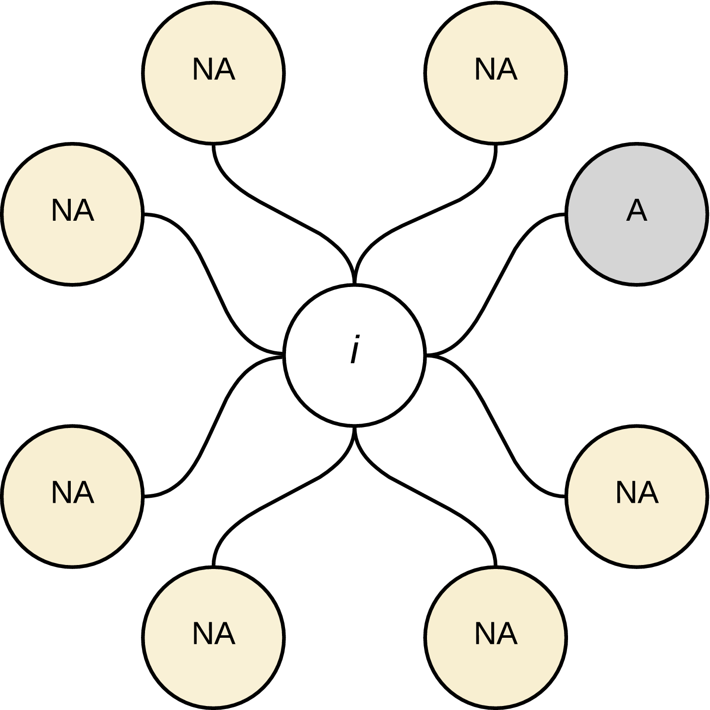
A Simple Social Network of Consumer i [Color figure can be viewed at wileyonlinelibrary.com]

Rational Observational Learning

Under the classical framework of rational observational learning, consumers try to infer product quality by observing all prior consumers' decisions, including many anonymous consumers (e.g., Banerjee 1992, Bikhchandani et al. 1992). In our example, consumer i needs to know all week 1 consumers' decisions to implement rational observational learning proposed in the literature. Suppose the vector of all week 1 consumers' decision is d = {d ₁, d ₂, ···, d _j, ···, d ₅₀}, where d _j indicates whether consumer j adopts the product (adopt: A; not adopt: NA). Under rational learning, consumer i's expost posterior is as follows:

\begin{matrix} Pr (V_{H} | d, S_{i}) = \\ \frac{Pr (d and S_{i} | V_{H}) Pr (V_{H})}{Pr (d and S_{i} | V_{H}) Pr (V_{H}) + Pr (d and S_{i} | V_{L}) Pr (V_{L})} \end{matrix},

where S _i is the private signal of consumer i. For simplicity, we assume that consumer i receives S _L. Therefore, under rational learning, the expected utility from the product is:

Pr (V_{H} | d, S_{i}) V_{H} + [1 - Pr (V_{H} | d, S_{i})] V_{L} .

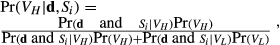
Cosumer i will adopt the product if the expected utility is greater than the price:

\Pr (V_{H} | d, S_{i}) V_{H} + [1 - \Pr (V_{H} | d, S_{i})] V_{L} e \frac{1}{2} V_{H} + \frac{1}{2} V_{L} .

In essence, the classical rational observational learning requires consumers to have extraordinary capability to acquire and process information: they need to have complete knowledge of all previous consumers' decisions and extract useful information from these decisions. However, in reality, consumers have limited time and attention to acquire and process information, and the cognitive capacity constraint limits the amount of information that they can acquire and process (Kahneman 2003). Behavioral observational learning based on friends' decisions can be thought of as reflecting a type of bounded rationality in which consumers are simply unable to acquire and make inferences from all prior consumers' decisions. In other words, behavioral observational learning is a simple and resonable decision rule based on friends' decisions.³

Behavioral Observational Learning

In this section, we propose a behavioral inference rule based on a focal consumer's friends' decisions. Now we consider consumer i's choice under our behavioral inference rule. When an early consumer in week 1 receives S _H, her posterior belief is as follows:

\Pr (V_{H} | S_{H}) = \frac{\Pr (S_{H} | V_{H}) \Pr (V_{H})}{\Pr (S_{H} | V_{H}) \Pr (V_{H}) + \Pr (S_{H} | V_{L}) \Pr (V_{L})} = 3 / 4,

and the expected utility is

\frac{3}{4} V_{H} + \frac{1}{4} V_{L}

, which is greater than the fixed price,

\frac{1}{2} V_{H} + \frac{1}{2} V_{L}

. When an early consumer in week 1 receives S _L, her posterior belief is as follows:

\Pr (V_{H} | S_{L}) = \frac{\Pr (S_{L} | V_{H}) \Pr (V_{H})}{\Pr (S_{L} | V_{H}) \Pr (V_{H}) + \Pr (S_{L} | V_{L}) \Pr (V_{L})} = 1 / 4,

and the expected utility is

\frac{1}{4} V_{H} + \frac{3}{4} V_{L}

, which is less than the fixed price,

\frac{1}{2} V_{H} + \frac{1}{2} V_{L}

. Therefore, when the firm charges an information‐revealing price, such as

\frac{1}{2} V_{H} + \frac{1}{2} V_{L}

, early consumers who receive S _H will adopt the propduct, and those who receive S _L will choose not to adopt.

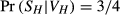
Let θ be the fraction of consumers who adopt the product over all consumers. If the product quality is V _H, then the fraction of consumers in week 1 who receive S _H is 3/4 because

\Pr (S_{H} | V_{H}) = 3 / 4

, and θ is (50/100) · (3/4) = 3/8. Note that 50% (50/100) of all consumers make their decisions in week 1 in our motivating example. If the quality is V _L, θ is (50/100) · (1/4) = 1/8.

On the basis of the information, we assume that consumer i performs a hypothesis test between two point hypotheses:

H_{0} : V = V_{H}; H_{1} : V = V_{L} .

If H ₀ is not rejected, consumer i thinks the product quality is V _H. If H ₀ is rejected, consumer i believes the quality is V _L. According to the Neyman–Pearson lemma (Casella and Berger 2002), the likelihood‐ratio test is uniformly most powerful (UMP) for testing simple hypotheses, so it is a test that has the highest power among all competitors. We use the following likelihood‐ratio test as consumers' decision rule:

Do not reject H ₀, if Λ > C; Reject H ₀, if Λ

\leq

where Λ is the ratio of the likelihood function, which will be specified later (a higher value of Λ means that the observed data is more likely to occur under the null hypothesis as compared with the alternative), and c is a constant, which is chosen to obtain a specified significance level, and 0 < c < 1. In our study, we choose a c to obtain a 5% significance level, which is very typical for hypothesis testing. Our results remain qualitatively similar if we choose a c to obtain a 1% or 10% significance level. The significance level reflects consumers' tolerance for type‐I error. Setting a 5% significance level in our decision rule means that the probability of rejecting the null hypothesis given that it is true is at or below 5%. Essentially, in the decision‐making process, consumers care about the number of friends who have purchased the product and the total number of friends. In the following paragraphs, we show that consumers adopt a cut‐off decision rule: If the number of friends who have purchased the product is greater than a threshold value, then they will decide to purchase the product. The threshold value is an increasing function of the total number of friends.

Our behavioral inference rule is intuitive, plausible, and tractable. First, the simple cut‐off decision rule is a cognitively simple and heuristic way for consumers to solve learning problems in a complex real‐world environment. The limited observability of consumers significantly complicate Bayesian updating and require extraordinary analytical and computational capabilities for a fully rational approach (Bala and Goyal 1998). It is highly impractical and cognitively demanding for an individual to observe all prior consumers' decisions and adopt Bayesian learning to do the required calculations (Kahneman 2003). Instead, we propose a fairly intuitive cut‐off decision rule, where consumers observe only their friends' decisions. The essence of our behavioral inference rule is consistent with the idea of procedural rationality proposed by Simon (1990): Procedural rationality is not an optimizing technique, but a heuristic method for arriving at satisfactory solutions with modest amounts of computation.

Second, the proposed behavioral inference rule based on a cut‐off strategy simply says that a consumer's decision depends on the relative popularity of a product. A growing stream of literature has discussed and proposed similar heuristic learning mechanisms to simplify Bayesian learning (Ellison and Fudenberg 1993, Eyster and Rabin 2010). For instance, Ellison and Fudenberg (1993) examined a non‐Bayesian social learning model in which people use a simple rule‐of‐thumb method based on the relative popularity of technologies to decide which technology they want to adopt. It is worth noting that an alternative naive learning mechanism is proposed by Golub and Jackson (2010). In their model, individuals average their estimates or beliefs with those of their friends. The key assumption is that individuals report their signals and opinions truthfully to their friends. This naive learning mechanism is not suitable for our context, because in observational learning, people observe the decisions of their friends instead of the beliefs of their friends. Although our cut‐off rule looks different from the rule proposed by Golub and Jackson (2010) on the surface, the spirit is similar: People who use the cut‐off rule actually average the decisions of their friends.

Additionally, the implication of our cut‐off decision rule is supported by empirical evidence in prior literature. Duan et al. (2009) empirically found that the relative popularity of products determines the timing and direction of observational learning. Finally, the optimal pricing problem in the presence of Bayesian observational learning is highly complex. Our behavioral inference rule makes the model analytically tractable.

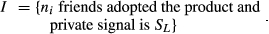
We assume that consumer i receives S _L, and the information set of consumer i is given by:

\begin{matrix} I & = {n_{i} friends adopted the product and \\ private signal is S_{L}} \end{matrix} .

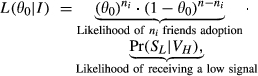
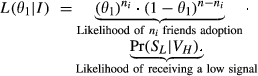
If the product quality is V _H, then θ = θ ₀ = 3/8. The likelihood of observing I in reality when the product quality is V _H is given by:

\begin{matrix} L (θ_{0} | I) & = \underset{Likelihood of n_{i} friends adoption}{\underset{⏟}{{(θ_{0})}^{n_{i}} \cdot {(1 - θ_{0})}^{n - n_{i}}}} \cdot \\ \underset{Likelihood of receiving a low signal}{\underset{⏟}{Pr (S_{L} | V_{H}),}} \end{matrix}

where n is the number of consumer i's friends, and n _i is the number of her friends who have adopted the product. The likelihood of observing I in reality when the product quality is V _L is given by:

\begin{matrix} L (θ_{1} | I) & = \underset{Likelihood of n_{i} friends adoption}{\underset{⏟}{{(θ_{1})}^{n_{i}} \cdot {(1 - θ_{1})}^{n - n_{i}}}} \cdot \\ \underset{Likelihood of receiving a low signal}{\underset{⏟}{Pr (S_{L} | V_{H}) .}} \end{matrix}

Λ is the ratio of the likelihood function when consumer i receives S _L and n _i of her friends adopted the product:

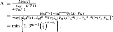
\begin{matrix} Λ & = \frac{L (θ_{0} | I)}{\sup_{θ \in {θ_{0}, θ_{1}}} L (θ | I)} \\ = \frac{{(θ_{0})}^{n_{i}} {(1 - θ_{0})}^{n - n_{i}} \Pr (S_{L} | V_{H})}{\max \{{(θ_{0})}^{n_{i}} {(1 - θ_{0})}^{n - n_{i}} \Pr (S_{L} | V_{H}), {(θ_{1})}^{n_{i}} {(1 - θ_{1})}^{n - n_{i}} \Pr (S_{L} | V_{L})\}} . \\ = \min \{1, 3^{n_{i} - 1} {(\frac{5}{7})}^{n - n_{i}}\} . \end{matrix}

(1)

The intuition for this decision rule is straightforward. The information that consumer i. observes is that she receives a private signal S _L, and n _i of her friends adopted the product. A higher value of Λ suggests that the observed data is more likely to occur under V = V _H as compared with V = V _L. Therefore, the decision rule for consumer i is a simple cut‐off strategy: When

n_{i} > n_{i}^{*} = \frac{\ln 3 c + (n) \ln (7 / 5)}{\ln (21 / 5)}

(the number of her friends who have adopted the product is greater than a threshold value), consumer i believes that the quality is V _H otherwise, the quality is V _L. In this example, the null hypothesis is V = V _H. In Appendix S3, we show that changing the null hypothesis to V = V _L does not make a qualitative difference in our analytical result.

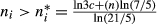
Suppose that all other things being equal, but consumer i receives S _H instead. Therefore, the information set of consumer i is I = {n _i friends adopted the product and private signal is S _H}. Following owing the same procedure, we can obtain the decision rule:

n_{i} > n_{i}^{*} = \frac{\ln c - \ln 3 + (n) \ln (7 / 5)}{\ln (21 / 5)} < \frac{\ln 3 c + (n) \ln (7 / 5)}{\ln (21 / 5)} .

It means that the threshold value when consumer i receives S _H is smaller than that when consumer i receives S _L. In other words, when consumer i receives a high signal S _H, she needs a smaller number of friends' adoption to justify that the product quality is high.

The aforementioned motivating example is oversimplified in an important way. The price charged by the firm is fixed. Some natural questions arise: What happens when prices are instead control variables? Could the seller manipulate the price to induce more purchases? In the next section, given that consumers adopt the behavioral inference rule, we study the optimal pricing strategy in the presence of observational learning in social networks.

Optimal Pricing under Different Learning Mechanisms in Social Networks

Model Setup

In this section, we study how a firm can use an information‐revealing pricing strategy to control the process of observational learning in social networks. Assume that a firm faces a unit measure of consumers, C = [0, 1], who are embedded in a social network. The degree of consumer i is the number of consumer i's friends, and each consumer has degree n. The equal degree assumption makes our model analytically tractable. This assumption is in line with the extant literature that has looked at similar modeling abstractions, such as Jackson (2008) and Qiu et al. (2016). Actually, in a large body of prior experimental studies on social networks, the equal degree assumption represents a balanced social network in reality and is a useful metaphor for many market environments (Carpenter et al. 2012, Charness et al. 2007, Qiu et al. 2014b, and Rosenkranz and Weitzel 2012). However, we do believe that relaxing equal degree assumption is important because it is difficult to envision that equal degree can fully mirror the circumstances of the environment of interest. We conduct additional numerical analyses to relax this assumption and introduce degree heterogeneity in Appendix S5.

Each consumer decides whether to adopt a product. The product is an experience good. It is common knowledge that the quality of the product is represented by a binary random variable: V ∈ {V _H, V _L}, and the true value of V is initially unknown to the buyers and the seller. In other words, we assume there is no asymmetric information between the buyers and the seller. This is a standard assumption in the literature on optimal pricing in the presence of learning (Bergemann and Valimaki 2006, Jing 2011a, Welch 1992). Another reason for adopting this assumption is to maintain the focus of observational learning. If the seller has some private information about the product quality, she might be able to signal this quality information through prices in a signaling game (Campbell 2015). As we focus on consumers' observational learning, we improve tractability by assuming that the seller has no private information. This assumption also captures the market information structure for experience products in reality. Li and Wang (2014) demonstrated that for experienced goods, such as music, video games, movies, and books, the firm and consumers are equally informed after the product launch because of open access to online product reviews.

We assume that all consumers are risk neutral, and the payoff function is V − P, where P is the price set by the firm. The pricing strategies will be specified later. All consumers share a common prior belief about the product quality:

\Pr (V_{H}) = α

, and

\Pr (V_{L}) = 1 - α

. Before each consumer makes a decision, she can access a binary private signal about the product quality. The signal can be either S _H or S _L, and satisfies:

\Pr (S_{H} | V_{H}) = \Pr (S_{L} | V_{L}) = q

\Pr (S_{L} | V_{H}) = \Pr (S_{H} | V_{L}) = 1 - q

, where 1/2 < q < 1. Note that q measures the precision of signals. q > 1/2 implies that if the product quality is V _H (V _L), the consumer is more likely to receive S _H (S _L). If q is higher, the signal is more informative.

It is worth noting that the binary signal structure is widely used in the observational learning literature in different fields, such as economics (Bikhchandani et al. 1992, Guarino et al. 2011), finance (Welch 1992), marketing (Iyer et al. 2007, Zhang et al. 2015), and information systems (Li and Wang 2014). One of the major advantages of a binary private signal structure is the analytical tractability. Smith and Sorensen (2000) showed that the binary signal structure can be extended to a signal with many possible realizations, but at significant algebraic cost. By assuming that the private information is either “high” or “low,” we are able to completely characterize the optimal pricing policy and focus on two pricing strategies that will be highlighted in our study: information‐revealing and pooling pricing strategies. In reality, the binary signal structure can be a simplified but useful approximation of the actual environment. A large stream of experimental literature has adopted the binary signal assumption (Alevy et al. 2007, Cipriani and Guarino 2005, Goeree et al. 2007). In real‐world situations, private quality information could come from a variety of sources. For instance, in digital music markets, a binary private signal can be interpreted as a consumer's perceived quality (positive or negative) when she observes the song title, the album title, the artist name, the album artwork, and any other visible information. A consumer can also form her own private opinions (positive or negative) on quality by reading online product reviews (such as Yelp.com) or third‐party professional reports (Chen and Xie 2005, Zhang et al. 2015).

We consider a dynamic model with two time periods. Assume that the firm is a monopoly and the marginal cost is a constant, which can be normalized to 0 without loss of generality. The monopolistic firm is risk neutral and maximizes the sum of profits in the two periods. To ease exposition, we ignore discounting in our model like Jing (2011b,c). At the beginning of period 1, the firm announces its pricing strategy,

(P_{1}, P_{2})

, where P _t is the price in period t, t = 1, 2. Also, we assume that the firm can credibly commit to second‐period prices. We adopt this assumption because of two reasons. First, in our model, the announced commitment prices maximize the firm's expected profits. Therefore, the firm has an incentive to use credible commitment to improve the expected profits. Second, price commitment on future prices is a common practice in reality as well as a widely adopted assumption in literature. Waldman (2003, p. 136) argued that: “commitments on future prices and quantities are common … analyses that assume no commitment at all is possible miss many of the important real‐world implications.” According to Jing (2011a), price commitment is a commonly used pricing strategy in daily life. For instance, future sales events (including the time duration and magnitudes of discounts) are routinely pre‐announced by retailers. Another example of price commitment is reality is limited‐time‐only offers: The special (usually lower) price is valid for a certain time window, beyond which the higher regular price resumes. The prior studies have investigated several price commitment devices used in practice. For instance, Cooper (1986) examined the most‐favored‐customer pricing policy: This policy is a promise by a firm that if it later lowers price, it will rebate to current customers the difference between the price they pay now and the lower future price. Butz (1990) analyzed a similar scheme, best‐price provisions, which guarantee that the price to be paid or received is the best available. If the seller subsequently cuts price, then each previous buyer is entitled to a refund. Choudhary (2007) also pointed out that money‐back guarantee is a plausible commitment device. On the other hand, a large stream of literature adopted the assumption that the firm can credibly commit to second‐period prices using one of many commitment devices (Choudhary 2007, Jing 2011a, Niculescu and Wu 2014, Waldman 2003, Zhang and Seidmann 2010).

The firm faces two groups of consumers: an initial group of early consumers and a group of late consumers. In period 1, fraction λ of all consumers, C ₁ = [0, λ], arrive and decide whether to adopt the product solely on the basis of the private signals they receive. We label them as early consumers. In period 1, consumer i's net payoff from adopting the product is V − P ₁. Early consumers adopt the product if the expected valuation is greater than the first period price. Following Banerjee (1992), we assume that early consumers are myopic and do not consider the strategic behavior of delaying the decision‐making process to obtain more information. In other words, the two groups of consumers act in an exogenously given order (Bikhchandani et al. 1992).

In period 2, fraction 1 − λ of all consumers, C ₂ = [λ, 1], make inferences about the quality and decide whether to adopt the product. We call these later decision makers late consumers. We consider two scenarios where late consumers follow the rational inference rule or the behavioral inference rule. As is standard in the observational learning literature (Bikhchandani et al. 1992, Smith and Sorensen 2000, Zhang et al. 2015), we assume a flat common prior α = 1/2 and the fraction λ = 1/2 without loss of generality. The analytical insights remain the same when λ ∈ (0, 1) and α ∈ (0, 1). In Appendix S2, we provide additional numerical analyses and show that our results are robust when we vary the value of exogenous parameters. Another reason we set α = 1/2 is that the role of observational learning is highlighted when the prior uncertainty is high. If α → 0 or 1, consumers are certain about the product quality and the impact of observational learning is insignificant. Setting the common prior, α, to be 1/2 is consistent with our assumption that the product is an experience good.

In our study, we assume that the proportion of early consumers in period 1, λ, is an exogenous parameter and is public information. First, this assumption is widely adopted in the prior economics and marketing literature for analytical tractability. For instance, Sun (2012) assumed a unit mass of early consumers enter the market in the first period, and another unit mass of late consumers enter the market in the second period. In particular, the seminal papers of observational learning (Banerjee 1992, Bikhchandani et al. 1992) have two working assumptions: (i) a sequence of consumers enter the market in an exogenous order (the sequence of decisions or the position of a consumer in the decision‐making queue is fixed and exogenous), which is equivalent to our assumption that the proportion of early consumers in period 1 is exogenous and fixed; and (ii) consumers have precise information about their position in the sequence of decisions (common knowledge), which is equivalent to our assumption that the proportion of early consumers in period 1 is public information shared by all consumers. These two working assumptions have been adopted by almost all observational learning models in diferent contexts in the past two decades (e.g., Acemoglu et al. 2011, Cao et al. 2011, Eyster and Rabin 2010, Guarino et al. 2011, Hendricks et al. 2012, Herrera and Hörner 2013, Moretti 2011, Moscarini et al.1998, Smith and Sorensen 2000, Zhang et al. 2015). Our assumption is consistent with the literature tradition and is an acceptable trade‐off for analytical tractability. It is worth noting that the exogenous λ (the proportion of early consumers in period 1) can be motivated by awareness effects. For example, in an observational learning model, Herrera and Hörner (2013) assumed that consumers randomly arrive and make decisions. Similarly, in our context, we can interpret the exogenous λ as some sort of awareness effects: a proportion of λ (randomly chosen) consumers becomes aware of the existence of the product and make their decisions in time period 1, and the rest are aware of the product in time period 2. The value of λ may reflect factors, such as firm‐side advertising, which are abstracted away in this model.

Second, our assumption is not only typical in consumer learning models, it is also realistic in many scenarios. In our model, when early consumers make their decisions, they do not need to know the proportion, λ. Only the firm and late consumers need to know it. In general, it is relatively easy for firms to obtain an estimate of λ by conducting consumer surveys (asking when consumers are likely to make their purchase decisions). However, consumers may also be able to have some rough ideas on λ from multiple information sources in different contexts. For instance, consumers may infer λ from survey results and reports in various popular consumer magazines, such as PC Magazine, PC World, and Consumer Reports, and a number of third‐party websites, such as CNET.com. Another example is an online market for music named Amie Street Music where users can listen to a sample of a song before they buy it at no monetary cost. They can also observe how many of other consumers have listened to the sample (potential consumers who are interested in the song) and the trend (Newberry 2016). These pieces of information can help consumers figure out λ. Similarly, in Amazon or Apple's App Store, the observable sales rank or download rank (over time) may help consumers infer the proportion of early consumers in period 1 (Chevalier and Goolsbee 2003, Garg and Telang 2013).⁴

Optimal Pricing Strategy under Rational Learning

We start with the rational learning scenario in which a subsequent consumer can observe all prior consumers' decisions. The key feature of rational observational learning is that a late consumer first observes the adoption decisions of all early consumers; then, upon the actions of all early consumers and her private signal, she infers the product quality using Bayesian updating and makes her own adoption decision. In this baseline scenario, there are two types of learning processes: (1) Private learning, in which early consumers learn from their private signals; and (2) rational observational learning, in which late consumers learn from all early consumers' decisions as well as their private signals. In period 1, if an early consumer receives a high signal, S _H, then her posterior belief becomes

μ_{H} = \Pr (V_{H} | S_{H})

. Similarly, if she observes a low signal, S _L, her posterior belief is:

μ_{L} = \Pr (V_{H} | S_{L})

The firm faces an optimal pricing problem: maximizing the expected profits by setting appropriate prices P ₁ and P ₂. The following lemma characterizes the possible locally optimal pricing strategies for the firm. All the proofs can be found in Appendix S1.

Lemma 1 Pricing Strategies under Rational Learning

Under rational observational learning and credible price commitment, the possible locally optimal pricing strategies for the firm are Strategy 1

{P_{1} = μ_{L} V_{H} + (1 - μ_{L}) V_{L}, P_{2} = μ_{L} V_{H} + (1 - μ_{L}) V_{L}};

Strategy 2

{P_{1} = μ_{L} V_{H} + (1 - μ_{L}) V_{L}, P_{2} = μ_{H} V_{H} + (1 - μ_{H}) V_{L}};

and Strategy 3

{P_{1} = μ_{H} V_{H} + (1 - μ_{H}) V_{L}, P_{2} = V_{H}} .

All other pricing strategies are strictly dominated by one of these three potential locally optimal pricing strategies.

Here, we provide a proof sketch of the lemma. In period 1, an early consumer either receives a high signal or a low signal. The willingness to pay of a consumer receiving a high signal is

μ_{H} V_{H} + (1 - μ_{H}) V_{L}

, and the willingness to pay of a consumer receiving a low signal is

μ_{L} V_{H} + (1 - μ_{L}) V_{L}

. If

P_{1} > μ_{H} V_{H} + (1 - μ_{H}) V_{L}

, no early consumers will adopt the product. If

μ_{L} V_{H} + (1 - μ_{L}) V_{L} < P_{1} \leq μ_{H} V_{H} + (1 - μ_{H}) V_{L}

, high signal consumers will choose to adopt the product. If 0

< P_{1} \leq μ_{L} V_{H} + (1 - μ_{L}) V_{L}

, all early consumers will adopt the product. Therefore, the optimal price in the first period could be either

P_{1} = μ_{H} V_{H} + (1 - μ_{H}) V_{L}

P_{1} = μ_{L} V_{H} + (1 - μ_{L}) V_{L}

Notice that

P_{1} = μ_{L} V_{H} + (1 - μ_{L}) V_{L}

and

P_{1} = μ_{H} V_{H} + (1 - μ_{H}) V_{L}

reflect two different pricing strategies. If

P_{1} = μ_{L} V_{H} + (1 - μ_{L}) V_{L}

, all early consumers will choose to adopt the product. The firm charges a price that does not reveal any information to late consumers. The decisions of early consumers contain no useful information about the quality to late consumers in period 2. In this case, a late consumer learns nothing by observing the choices of their friends, and make inferences about the quality by her own signal only. It is equivalent to a pricing strategy in the absence of observational learning. We call pricing strategies 1 and 2 the pooling pricing strategy. Under the pooling pricing strategy, the optimal price in the second period is still

P_{2} = μ_{H} V_{H} + (1 - μ_{H}) V_{L}

P_{2} = μ_{L} V_{H} + (1 - μ_{L}) V_{L}

P_{1} = μ_{H} V_{H} + (1 - μ_{H}) V_{L}

, early consumers who receive S _H will adopt the product, and those receiving S _L will not. In the presence of rational learning, a late consumer will know the quality by observing all early consumers' choices. We call it the information‐revealing pricing strategy. Under information‐revealing pricing strategy, the optimal price in period 2 could be either P ₂ = V _H or P ₂ = V _L. In particular, the pricing strategy

{P_{1} = μ_{H} V_{H} + (1 - μ_{H}) V_{L}, P_{2} = V_{L}}

is strictly dominated by the pricing strategy

{P_{1} = μ_{H} V_{H} + (1 - μ_{L}) V_{L}, P_{2} = μ_{H} V_{H} + (1 - μ_{H}) V_{L}} .

We characterize the optimal pricing strategy under rational learning in the following proposition.

Proposition 1 Optimal Pricing Strategy under Rational Learning

Under rational learning and credible price commitment, (i) if

V_{H} / V_{L} \geq \frac{\frac{5}{4} q - \frac{1}{4}}{\frac{5}{4} q - \frac{3}{4}}

and

\frac{3}{5} <

q < 1, the information‐revealing pricing strategy 3

{P_{1} = μ_{H} V_{H} + (1 - μ_{H}) V_{L}, P_{2} = V_{H}},

is optimal for the firm; if

1 < V_{H} / V_{L} < \frac{\frac{5}{4} q - \frac{1}{4}}{\frac{5}{4} q - \frac{3}{4}}

and

\frac{3}{5} <

q < 1; or

\frac{1}{2} < q \leq \frac{3}{5}

, the pooling pricing strategy 1

{P_{1} = μ_{L} V_{H} + (1 - μ_{L}) V_{L}, P_{2} = μ_{L} V_{H} + (1 - μ_{L}) V_{L}},

is optimal for the firm. Furthermore, (ii) when q is higher, the information‐revealing pricing strategy is optimal in a wider range of the parameter space of V _H/V _L; (iii) when V _H/V _L is higher, the information‐revealing pricing strategy is optimal in a wider range of the parameter space of q.

A proof sketch is provided as follows. According to Lemma 1, we have three possible pricing strategies. We compare the firm's profits under three different pricing strategies and the result follows. The proposition implies that when the private signal is sufficiently noisy (

\frac{1}{2} < q \leq \frac{3}{5}

), it is uniquely optimal for the firm to use the pooling pricing strategy. Instead when the signal is sufficiently precise (

\frac{3}{5} < q < 1

), the optimal pricing strategy depends crucially on the ratio V _H/V _L.

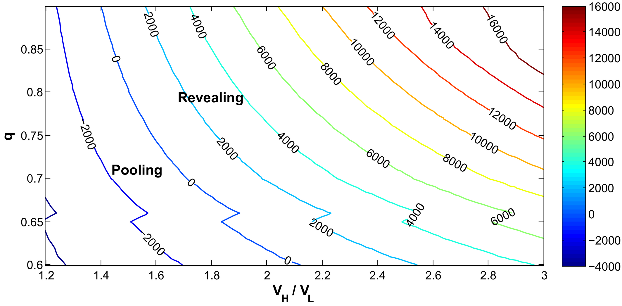
To provide some additional intuition, we conduct a numerical analysis and visualize Proposition 1 in Figure 2. For simplicity, we assume there are 10,000 consumers in both period 1 and period 2. The profits of pricing strategies 1, 2, and 3 under rational learning are represented by π ₁, π ₂, and π ₃, respectively. We define the difference between the profits generated by the information‐revealing pricing strategy and the pooling pricing strategy as π ₃ − max{π ₁, π ₂}. Figure 2 depicts the contour lines of the profit difference for different values of the precision of the private signal, q, and the ratio V _H/V _L. Note that the contour level‐0 line means the profit difference is 0. Therefore, the whole region can be divided by this contour line. When the profit difference is less than 0, the firm should use the pooling pricing strategy. When the profit difference is greater than 0, the firm should use the information‐revealing pricing strategy.

Figure 2

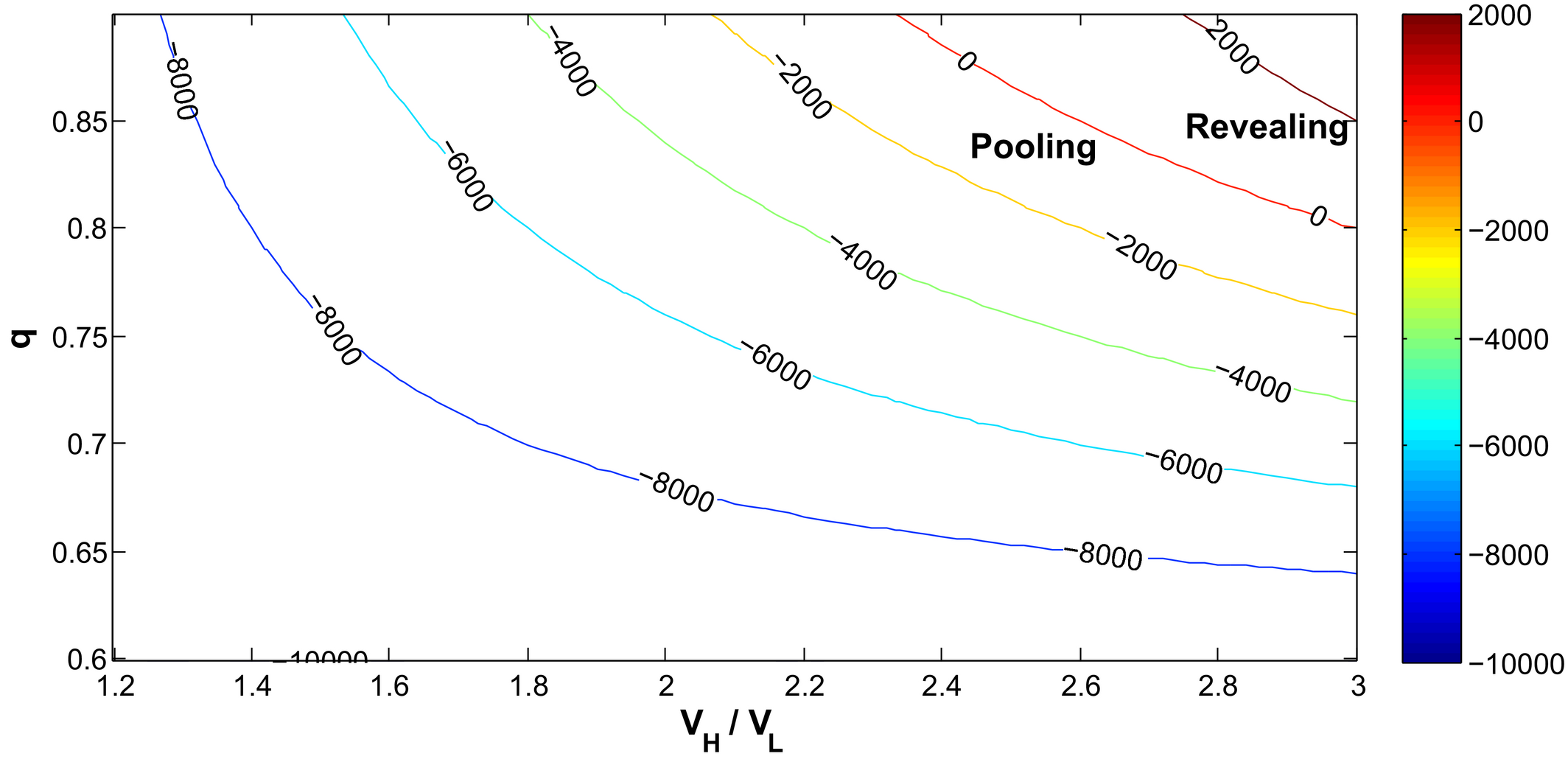
Profit Comparison of Different Pricing Strategies under Rational Learning [Color figure can be viewed at wileyonlinelibrary.com]

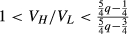
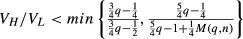
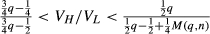
As for result (ii) in Proposition 1, we increase the value of q and examine its impact on the parameter space of V _H/V _L in which the information‐revealing pricing strategy is optimal. When q = 0.6, the information‐revealing strategy is never optimal no matter what the value of V _H/V _L is; when q = 2/3, the information‐revealing strategy is preferred when

\frac{V_{H}}{V_{L}} \in [7, + \infty];

when q = 0.7, the information‐revealing strategy is preferred when

\frac{V_{H}}{V_{L}} \in [5, + \infty];

and when q = 0.8, the information‐revealing strategy is preferred when

\frac{V_{H}}{V_{L}} \in [3, + \infty] .

From this numerical example, we can see that when q is higher, the information‐revealing pricing strategy is optimal in a wider range of the parameter space of V _H/V _L. We can think of the value of V _H/V _L as a specific market condition. Our proposition implies that the use of information‐revealing pricing strategy is optimal in a wider range of market conditions when q is higher.

The implication of result (iii) is similar: When V _H/V _L = 2, the information‐revealing strategy is never optimal no matter what the value of q is; when V _H/V _L = 3, the information‐revealing strategy is preferred when q ∈ [0.8, 1]; and when V _H/V _L = 5; the information‐revealing strategy is preferred when q ∈ [0.7, 1]. Similarly, we can see that when V _H/V _L is larger, the information‐revealing pricing strategy is optimal in a wider range of the parameter space of q. In other words, the use of information‐revealing pricing strategy is optimal in a wider range of market conditions when V _H/V _L is larger.

Note that in Figure 2, our parameter choice,

\frac{V_{H}}{V_{L}} \in [1.2, 3]

and q ∈ [0.6, 0.9], covers a large range of possible parameter values in reality, so the numerical approach does not sacrifice generalizability in our context. The numerical results show that under rational learning, the use of the information‐revealing pricing strategy should be limited in a fairly small range of market conditions. Only in extreme market conditions should the firm adopt the information‐revealing pricing strategy under rational learning: For instance, in prior experimental studies on observational learning, various reasonable values of signal precision q were picked. In Hung and Plott (2001), and Alevy et al. (2007),

q = \frac{2}{3}

, and in this case, the information‐revealing strategy is preferred when V _H/V _L ≥ 7 according to Proposition 1, which is an extremely large quality difference. In Cipriani and Guarino (2005), q = 0.7, and the information‐revealing strategy is preferred when V _H/V _L ≥ 5. Goeree et al. (2007) chose

q = \frac{5}{9}

, and in this case, the information‐revealing strategy is always dominated by the pooling strategy no matter how large V _H/V _L is. In Noth and Weber (2003), q is chosen to be 0.6 or 0.8. When q = 0.6, the information‐revealing strategy is never optimal; and when q = 0.8, the information‐revealing strategy is preferred when V _H/V _L ≥ 3. In sum, the results under rational learning suggest that the pooling pricing strategy is optimal for the firm in most of the cases the market is likely to experience.

Optimal Pricing Strategy under Behavioral Learning

Under behavioral observational learning, we relax the assumption of rational learning, in which a late consumer can observe all early consumers' decisions. In this section, a late consumer first observes the decisions of her friends; then, upon the actions of her friends and her private signals, they follow the behavioral inference rule proposed in section 3.3. For simplicity, we consider a regular social network, where every consumer has the same degree n (Jackson 2008). Following Galeotti and Goyal (2009), we assume that consumers believe that the friendship formation is a random sampling process. This assumption avoids complicated inference. Each consumer randomly draws n consumers as her friends from all consumers. In other words, each consumer chooses a n‐sized sample: she makes n draws, and each draw is independent from each other. Note that n measures the level of social interactions, and a higher n means a denser social network. Consumer i observes the number of her friends who adopted the product, n _i.

As is discussed in the section of rational learning, the firm can use two types of pricing strategies depending on whether all early consumers adopt the product in period 1. If a pricing strategy is used such that all early consumers adopt the product in period 1, a late consumer will learn nothing from her friends' decisions, and the pricing strategy is information pooling. If a pricing strategy is used such that some early consumers adopt the product in period 1 but some do not, a late consumer will be able to infer the product quality from her friends' decisions, and the pricing strategy is information revealing.

Similar to the rational learning scenario, there are two types of learning processes under behavioral observational learning: (1) Private learning, in which early consumers learn from their private signals; and (2) behavioral observational learning, in which late consumers learn from early friends' decisions as well as their private signals. In the following lemma, we show that a late consumer's inference rule under behavioral observational learning is a simple cut‐off strategy when an information‐revealing pricing strategy is used. When a pooling pricing strategy is adopted, a late consumer will focus only on her private signal because no quality information is revealed in period 1.

Lemma 2 Inference Rule under Behavioral Learning

Under behavioral learning, a late consumer's inference rule when the firm adopts an information‐revealing pricing strategy is as follows: A late consumer i who receives S _H will infer that the product quality is V _H if n _i is greater than a threshold

n_{H}^{*}

and that it is V _L otherwise; a late consumer i who receives S _L will infer that the product quality is V _H if n _i is greater than a threshold

n_{L}^{*}

and that it is V _L otherwise. A late consumer's inference rule when the firm adopts a pooling pricing strategy is to ignore the decisions of her friends and rely on her private signal only.

We provide a proof sketch as follows. If the firm adopts a pooling pricing strategy, a late consumer learns nothing from friends' deicsions. If the firm adopts a revealing pricing strategy (

P_{1} = μ_{H} V_{H} + (1 - μ_{H}) V_{L}

), early consumers who receive S _H will adopt the product. Late consumers can update the prior belief by employing observational learning, and then they use the hypothesis testing rule. In the lemma, the threshold degrees

n_{H}^{*}

and

n_{L}^{*}

are functions of signal precision q and network size n. The details of the functional forms of

n_{H}^{*} (q, n)

and

n_{L}^{*} (q, n)

are specified in Appendix S1. Since the friendship formation is a random sampling process, n _i follows a binomial distribution, which is given by the probability mass function:

\Pr (n_{i} = n_{a}) = (\begin{matrix} n \\ n_{a} \end{matrix}) θ^{n_{a}} {(1 - θ)}^{n - n_{a}}

, where θ is the proportion of early consumers who adopted the product among all consumers, which depends on the first period price, P ₁. For late consumers who receive S _H, a proportion of them,

β_{H} (θ, q, n)

, believes the product quality is V _H, where

β_{H} (θ, q, n) = \sum_{n_{a} > n_{H}^{*} (q, n)} P r (n_{i} = n_{a}) .

Similarly, For late consumers who receive S _L, a proportion of them,

β_{L} (θ, q, n)

, believes the product quality is V _H, where

β_{L} (θ, q, n) = \sum_{n_{a} > n_{L}^{*} (q, n)} P r (n_{i} = n_{a}) .

Following a similar argument in the proof sketch of Lemma 1, we can obtain the following result: Under behavioral learning and credible price commitment, the possible locally optimal pricing strategies for the firm are strategy 1,

{P_{1} = μ_{L} V_{H} + (1 - μ_{L}) V_{L}, P_{2} = μ_{H} V_{H} + (1 - μ_{H}, P_{2} = μ_{H} V_{H} + (1 - μ_{H}) V_{L}};

strategy 2,

{P_{1} = μ_{L} V_{H} + (1 - μ_{L}) V_{L}, P_{2} = μ_{H} V_{H} + (1 - μ_{H}, P_{2} = μ_{H} V_{H} + (1 - μ_{H}) V_{L}};

and strategy 3,

{P_{1} = μ_{H} V_{H} + (1 - μ_{H}) V_{L}, P_{2} = V_{H}} .

All other pricing strategies are strictly dominated by one of these three potential locally optimal pricing strategies. Similarly, pricing strategies 1 and 2 are pooling pricing strategies, and pricing strategy 3 is an information‐revealing pricing strategy. Information‐revealing pricing strategy only works well under certain conditions. It is worth noting that the set of the potential locally optimal pricing strategies under rational observational learning (Lemma 1) is the same set of strategies under behavioral observational learning. The reason is that no learning occurs in period 1, and the possible optimal price in period 1 is either

P_{1} = μ_{L} V_{H} + (1 - μ_{L}) V_{L}

P_{1} = μ_{H} V_{H} + (1 - μ_{H}) V_{L}

under both learning mechanisms. Under the pooling strategy (

P_{1} = μ_{L} V_{H} + (1 - μ_{L}) V_{L}

), no information is revealed by the pruchase decisions of early consumers, so the case under rational observational learning is equivalent to that under behavioral observational learning. Under the revealing strategy (

P_{1} = μ_{H} V_{H} + (1 - μ_{H}) V_{L}

), late consumers learn differently under the two learning mechanisms. The learning results differ in the proportion of late consumers who think the product quality is high. However, both rational and behavioral learning mechanisms lead to a similar pattern: a proportion of late consumers will think that the product quality is high, and the rest will think that the product quality is low. Therefore, the set of the potential locally optimal pricing strategies is the same under both rational and behavioral learning mechanisms.

A natural question arises: When does the use of information‐revealing pricing strategy increase the profits of the firm? We first provide a numerical example, presented in Figure 3, to offer some intuition. We set the number of friends of each consumer to n = 10. Note that n should be small relative to the number of consumers in period 1. That is the key point of relaxing the assumption in rational learning: people observe only their friends' decisions instead of all of the choices made by prior consumers. For the behavioral decision rule based on hypothesis testing, we choose a c to obtain a 5% significance level. Like the numerical analysis in rational learning, we assume there are 10,000 consumers in both period 1 and period 2. Similarly, the profits under pricing strategies 1, 2, and 3 are represented by π ₁, π ₂, and π ₃, respectively. Figure 3 depicts the contour lines⁵ of the profit difference π ₃ − max{π ₁, π ₂} for different values of the precision of the private signal, q, and the ratio V _H/V _L. This numerical example shows that when q and V _H/V _L are large, the use of information‐revealing pricing strategy increases the profits of the firm. When q becomes larger, the private signal is more informative. When V _H/V _L is large, the uncertainty of product quality is high. Under both cases, it is more valuable to observe other consumers' choices. In other words, observational learning is more effective in increasing the consumers' willingness to pay. Thus, pricing strategy 3 dominates the pooling pricing strategy. More importantly, Figure 3 shows that under behavioral learning, the firm should adopt the information‐revealing pricing strategy in a wide range of market conditions.

Figure 3

Profit Comparison of Different Pricing Strategies under Behavioral Learning

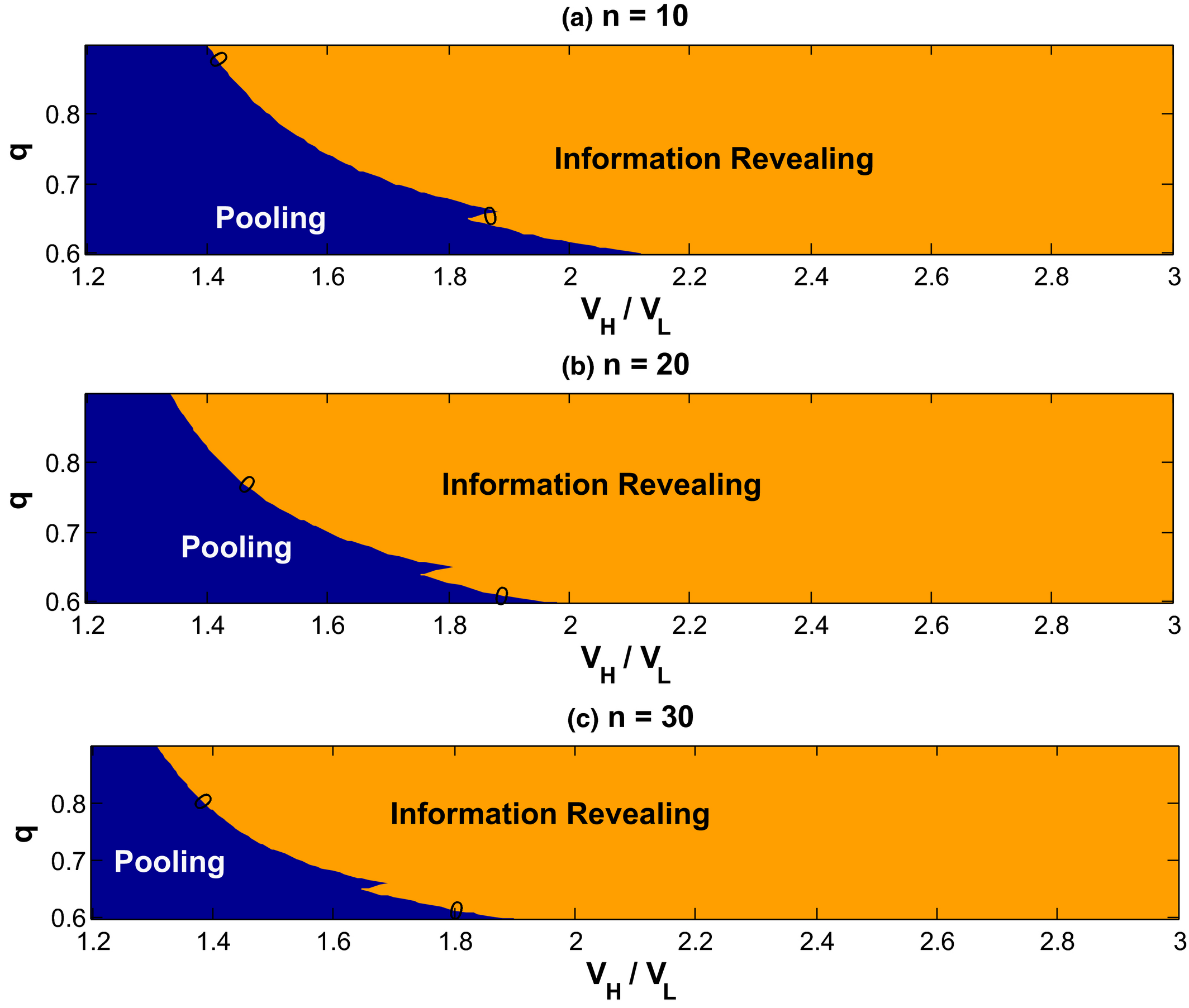
We also examine the effect of network density, n, on the choice of optimal pricing strategies. In Figure 4, we depict the contour lines of the profit difference, π ₃ − max{π ₁, π ₂}, when the network density varies (n = 10, 20, 30), and indicate the region where the information‐revealing or pooling pricing strategy is optimal. Recall that in reality, the network density n should be small relative to the total number of consumers. We find that the use of information‐revealing pricing strategy is optimal in a wider range of market conditions when the network is denser (given that n is relatively small). However, when n is large, an increase in n makes the information revealing strategy less optimal. In our current parameter setup, we find that the upper limit of the network density is

\bar{n} = 862 .

When

n < \bar{n},

the use of information‐revealing pricing strategy is optimal in a wider range of market conditions when the network is denser (see Figure 4). However, as shown in Figure 5, when

n \geq \bar{n},

an increase in n makes the information revealing strategy less optimal.

Figure 4

The Effect of Network Density on the Choice of Optimal Pricing Strategies under Behavioral Learning (n is Small) [Color figure can be viewed at wileyonlinelibrary.com]

Figure 5

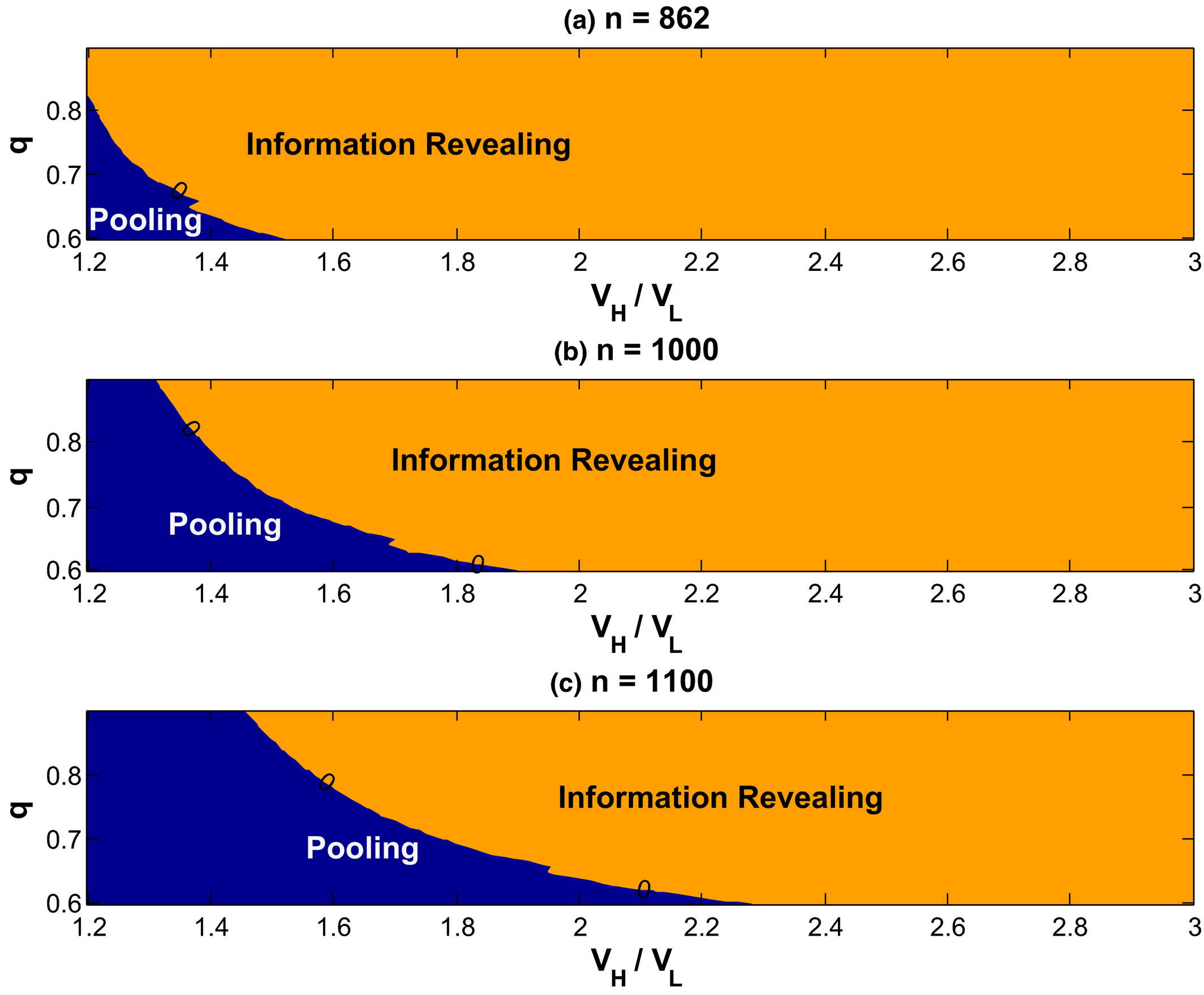
The Effect of Network Density on the Choice of Optimal Pricing Strategies under Behavioral Learning (n is Large) [Color figure can be viewed at wileyonlinelibrary.com]

There are two underlying trade‐off forces that make

\bar{n}

exist. On the one hand, when the consumer degree n is larger, learning plays a more important role in such a denser network. Therefore, information‐revealing pricing strategy tend to dominate the pooling pricing strategy in a wider range of market conditions. However, on the other hand, there is another opposite force: when n becomes larger, the inference rule under behavioral learning becomes more similar to that under rational learning. An extreme case is that n equals the total number of consumer in the first period. In this case, a late consumer can observe all early consumers' decisions, which is equivalent to the scenario in rational observational learning. Under rational learning, if the firm adopts the information‐revealing pricing strategy, a late consumer in period 2 can observe the decisions of all consumers in period 1, and hence will discover the true product quality. In other words, the learning is perfect. As shown in the literature, prefect learning does not always benefit the firm (Yu et al. 2015). In our context, perfect learning is not consistent with the profit maximization objective of the firm except when V _H/V _L is high. Therefore, if the second force dominates, an increase in n makes the information revealing strategy less optimal. Specifically, the second force is more likely to dominate the first force when n is very large because of two reasons: (i) The magnitude of the first force decreases when n is larger. Essentially, the marginal value of additional information from friends is decreasing. (ii) The second force is stronger when n is larger. In other words, a larger n makes the scenario more similar to the rational observational learning case.

In particular, it is worth noting that in reality, the first underlying force usually dominates the second one because the degree n should be very small relative to the total number of consumers in the first period. For example, the number of potential consumers for a product could be in millions, but the social network degree for an ordinary consumer is just in hundreds. In Figure 4, n = 10, and the total number of consumers in the first period is 10,000. Therefore, the first force dominates, and we find that the use of information‐revealing pricing strategy is optimal in a wider range of market conditions when the network is denser (it holds as long as

n \geq \bar{n} = 862,

). Only when

n \geq \bar{n} = 862,

the second force dominates, but this scenario is not very likely in the real world (especially for popular products) because it implies that more than 8.62% (862/10,000) of the total potential customers in the first period are friends of a late consumer in the second period. Such a dense network may exist only for some particular niche products.

In the following proposition, we generalize the numerical results and describe the optimal pricing strategies under different market conditions, followed by a discussion of the managerial implications. For notational simplicity, let

\begin{matrix} M (q, n) & = q [β_{H} (θ = \frac{q}{2}, q, n) + β_{H} (θ = \frac{1 - q}{2}, q, n)] \\ + (1 - q) [β_{L} (θ = \frac{q}{2}, q, n) + β_{L} (θ = \frac{1 - q}{2}, q, n)] \end{matrix} .

Proposition 2 Information‐Revealing vs. Pooling

Under behavioral learning and credible price commitment, the information‐revealing pricing strategy 3, {P ₁ = μ _H V _H + (1 − μ _H)V _L, P ₂ = V _H} is optimal for the firm if (i)

\frac{1}{2} < q \leq \frac{2}{3}

and

V_{H} / V_{L} \geq \frac{\frac{5}{4} q - \frac{1}{4}}{\frac{5}{4} q - 1 + \frac{1}{4} M (q, n)}

; or (ii)

q > \frac{2}{3}

and

\frac{\frac{5}{4} q - \frac{1}{4}}{\frac{5}{4} q - 1 + \frac{1}{4} M (q, n)} \leq V_{H} / V_{L} \leq

\frac{\frac{3}{4} q - \frac{1}{4}}{\frac{3}{4} q - \frac{1}{2}}

; or (iii)

q > \frac{2}{3}

and

V_{H} / V_{L} \geq m a x \{\frac{\frac{3}{4} q - \frac{1}{4}}{\frac{3}{4} q - \frac{1}{2}}, \frac{\frac{1}{2} q}{\frac{1}{2} q - \frac{1}{2} + \frac{1}{4} M (q, n)}\}

. The pooling pricing strategy 1, {P ₁ = μ _L V _H + (1 − μ _L)V _L, P ₂ = μ _L V _H + (1 − μ _L)V _L}, is optimal for the firm if (iv)

\frac{1}{2} < q \leq \frac{2}{3}

and

V_{H} / V_{L} < \frac{\frac{5}{4} q - \frac{1}{4}}{\frac{5}{4} q - 1 + \frac{1}{4} M (q, n)}

; or (v)

q > \frac{2}{3}

and

V_{H} / V_{L} < m i n \{\frac{\frac{3}{4} q - \frac{1}{4}}{\frac{3}{4} q - \frac{1}{2}}, \frac{\frac{5}{4} q - \frac{1}{4}}{\frac{5}{4} q - 1 + \frac{1}{4} M (q, n)}\}

. The pooling pricing strategy 2, {P ₁ = μ _L V _H + (1 − μ _L)V _L, P ₂ = μ _H V _H + (1 − μ _H)V _L}, is optimal for the firm if (vi)

q > \frac{2}{3}

and

\frac{\frac{3}{4} q - \frac{1}{4}}{\frac{3}{4} q - \frac{1}{2}} < V_{H} / V_{L} < \frac{\frac{1}{2} q}{\frac{1}{2} q - \frac{1}{2} + \frac{1}{4} M (q, n)}

A proof sketch is provided as follows. We only need to compare the profits under the three different pricing strategies mentioned earlier. For pricing strategies 1 and 2 that do not induce observational learning, late consumers do not update the prior belief by observing the decisions of their friends. For pricing strategy 3 that induces observational learning, late consumers use the behavioral inference rule to make their decisions. From Lemma 2, we know how to compute

β_{H} (θ, q, n)

and

β_{L} (θ, q, n)

, and the result follows.

Proposition 2 characterizes under what market conditions information‐revealing or pooling pricing strategy is optimal in the presence of behavioral learning. There are two trade‐offs in choosing the pooling or information‐revealing pricing strategy: (1) The monopoly faces a downward sloping demand curve. We assume that the monopolist firm cannot make price discrimination to gain more profit. In other words, the firm can charge only one price. By raising P ₁, the firm will lose some business in period 1. (2) The trade‐off associated with observational learning and information pooling. In social networks, consumers can observe the decisions of their friends. Hence, the firm can control the information available to late consumers by charging different prices. It is the crucial trade‐off on which our model focuses. If the firm charges

P_{1} = μ_{L} V_{H} + (1 - μ_{L}) V_{L}

, the low price does not reveal any information to late consumers. When the value of observational learning is large, the firm benefits from charging a high price,

P_{1} = μ_{H} V_{H} + (1 - μ_{H}) V_{L}

, which reveals information to late consumers.

Optimal Pricing Strategy under Rational Learning Vs. Behavioral Learning

In this section, we compare optimal pricing strategy under rational learning with that under behavioral learning and obtain several important insights on what the corresponding optimal pricing strategies are. In Figures 2 and 3, we find that the information‐revealing pricing strategy is optimal only in extreme market conditions under rational learning. However, under behavioral learning, the use of information‐revealing pricing strategy is optimal in a wide range of market conditions. For instance, when q = 0.75, the information‐revealing pricing strategy is never optimal under rational learning no matter how large V _H/V _L is. However, under behavioral learning, the information‐revealing pricing strategy is optimal when V _H/V _L ≥ 1.6. In other words, behavioral learning makes the information‐revealing pricing strategy optimal for the seller with a much lower threshold value of V _H/V _L.

Why do the optimal pricing polices differ under rational learning and behavioral learning? The key underlying intuition is that under rational learning, if the firm adopts the information‐revealing pricing strategy, a late consumer in period 2 can observe the decisions of all consumers in period 1, and hence will discover the true product quality. However, in our context, perfect learning is not consistent with the profit maximization objective of the firm except when V _H/V _L is high. Recall that as is standard in the literature (Bergemann and Valimaki 2006, Jing 2011a, Welch 1992), there is no asymmetric information about product quality between the buyers and the seller in our model. In other words, the firm is not completely certain about the product quality. When V _H/V _L is high, the firm can charge a high price if consumers know that the product quality is V _H. Therefore, perfect learning benefits the firm in the case that V _H/V _L is high. However, when V _H/V _Lis moderate or low, the benefit of perfect learning is lower. On the other hand, the risk of perfect learning comes from the fact that it may reveal the true product quality if the product quality is V _L. Therefore, we can obtain: (i) under rational learning, information pooling is optimal when V _H/V _L is moderate or low.

Under behavioral learning, the region in which information pooling is optimal is smaller than that under rational learning. In contrast with rational learning, behavioral learning is not perfect learning, but still better informs consumers about product quality. In other words, under behavioral learning, information‐revealing strategy will help consumers know the product quality more precisely, but it will not reveal the product quality perfectly. Therefore, the risk of learning (the low quality is revealed) is lower, and it makes the information‐revealing strategy optimal for the seller in a wider range of market conditions with a much lower threshold value of V _H/V _L. We can obtain: (ii) Under behavioral learning, information pooling is optimal only when V _H/V _L is low. Combined (i) with (ii), we know that the region in which information pooling is optimal under behavioral learning is a proper subset of the region in which information pooling is optimal under rational learning (shown in Figures 2 and 3).

Our model has implications for how a manager can develop more effective pricing strategies in social networks. If a firm insists the full rationality assumption in which a consumer can observe all of her predecessors' choices, the pooling pricing strategy will be adopted in most of the cases. Our analytic insights suggest that in a more realistic rationality assumption, the information‐revealing pricing strategy can increase the firm's profits, and hence should be more widely adopted. It is worth noting that the managerial implication of our model is different from that of the seeding literature. Introductory discounts and a free demonstration to a targeted group of consumers are widely used as methods to boost adoption. Jing (2011b) studied seller‐induced learning, such as sponsoring test use, offering product demonstration and training seminars, in a durable goods market. Ho et al. (2012) showed that a firm can amplify social contagion and accelerate product purchases by offering introductory discounts. However, in our model, a low price in period 1 implies a pooling pricing strategy, which results in no information revelation to the new consumers in networks. Offering introductory discounts is not always an effective method to boost purchases. It could be detrimental to social contagion and product adoption. Similarly, Dey et al. (2013) examined the effect of consumer learning on the design of free software trials and found that a free trial may not be optimal in many practical situations. In our model, consumers make inferences about the quality according to the actions of their friends. Introductory discounts actually prevent observational learning that could increase the new consumers' willingness to pay. Thus, our model suggests that introductory discounts might not be an optimal pricing strategy under the circumstances in which behavioral observational learning plays an important role.

Conclusions and Future Research Directions

In the present study, we explored the optimal pricing in the presence of behavioral observational learning. The monopolist controls the speed of observational learning, using different pricing strategies. Our study offers some important managerial implications. We find that local merchants can benefit from the informative pricing strategy that results in more observational learning in social networks. Surprisingly, introductory discounts could prevent observational learning and reduce the monopoly profits under some circumstances.

Several additional steps can be taken to examine observational learning and optimal pricing in social networks. First, the firm in our model is assumed to be a monopoly. A future research direction would be to examine the competition effects, using the standard Hotelling model (Cheng et al. 2011). Second, following the literature (Niculescu and Wu 2014), we retained the credible price commitment framework. It would be interesting to relax this assumption in our future research. Third, following the prior literature on observational learning (Acemoglu et al. 2011, Banerjee 1992, Bikhchandani et al. 1992, Smith and Sorensen 2000), we assumed that all consumers share the same opinion on vertical quality in our model. However, we do realize that horizontal taste difference (consumers have different tastes) is a very important dimension of consumer preference. Chen and Xie (2005) differentiate between two types of consumers: “taste‐driven” and “quality‐driven” consumers. Essentially, we assume that the consumers in our model are quality‐driven consumers. A future research direction of our model is to allow products to differ in two dimensions: quality (vertical) dimension and taste (horizontal) dimension. Fourth, our analytical model focused on the channel of observational learning; however, in reality, consumers might contact their friends who adopted the product to figure out how well they liked it (word of mouth). It would be natural to examine different channels of social contagion, such as observational learning and word of mouth, in a unified analytical model. Finally, we did not allow price discrimination in the present model. We could relax this assumption and consider the use of price discrimination on the basis of social network structures, such as targeting consumers having high centrality measures.

Footnotes

Acknowledgments

The authors thank the department editor, the senior editor, and three anonymous reviewers for their detailed and constructive comments. The authors also thank Maxwell Stinchcombe, Thomas Wiseman, De Liu, Ying‐Yu Chen, and the participants of the 2012 INFORMS Conference on Information Systems and Technology (CIST) for helpful feedback.

1

The detailed difference between payoff externalities and information externalities can be found in Moretti (2011) and Qiu et al. ().

2

An assumption of our model is that all consumers share the same utility function.

3

It is worth noting that even if consumer i in our example wants to conduct rational learning based on friends' decisions, it would be very complicated because she does not know other early consumers' decisions. She could form an expectation on all other early consumers' decisions, but there are 2^N possibilities, where N is the number of early consumers in week 1 whose decisions are not observed by consumer i. It is a high rationality requirement to compute the expected utility based on all possible cases.

4

We may also consider an example of consumers deciding whether to buy a newly released smartphone, such as the newest model of iPhone. Consumers make this decision when their existing service contracts expire, so that there is an exogenous sequence of actions determined by contracts. In this context, each consumer may observe the choices of her friends, neighbors, and coworkers.

5

The discontinuity in contour line is caused by the discontinuity (in q = 2/3) of the conditions for the information‐revealing pricing strategy to be optimal, as described in Proposition .

References

Acemoglu

Dahleh

M. A.

Lobel

Ozdaglar

. 2011. Bayesian learning in social networks. Rev. Econ. Stud. 78(4): 1201–1236.

Alevy

J. E.

Haigh

M. S.

List

J. A.

. 2007. Information cascades: Evidence from a field experiment with financial market professionals. J. Finance 62(1): 151–180.

August

Niculescu

M. F.

. 2013. The influence of software process maturity and customer error reporting on software release and pricing. Management Sci. 59(12): 2702–2726.

Bala

Goyal

. 1998. Learning from neighbours. Rev. Econ. Stud. 65(3): 595–621.

Banerjee

1992. A simple model of herd behavior. Q. J. Econ. 107(3): 797–817.

Bendoly

Croson

Goncalves

Schultz

. 2010. Bodies of knowledge for research in behavioral operations. Prod. Oper. Manag. 19(4): 434–452.

Bergemann

Valimaki

. 2006. Dynamic pricing of new experience goods. J. Polit. Econ. 114(4): 713–743.

Bikhchandani

Hirshleifer

Welch

. 1992. A theory of fads, fashion, custom, and cultural change in informational cascades. J. Polit. Econ. 100(5): 992–1026.

Butz

D. A.

1990. Durable‐good monopoly and best‐price provisions. Am. Econ. Rev. 80(5): 1062–1076.

10.

Campbell

J. D.

2015. Localized price promotions as a quality signal in a publicly observable network. Quant. Market. Econ. 13(1): 27–57.

11.

Cao

H. H.

Han

Hirshleifer

. 2011. Taking the road less traveled by: Does conversation eradicate pernicious cascades? J. Econ. Theory 146(4): 1418–1436.

12.

Carpenter

Kariv

Schotter

. 2012. Network architecture, cooperation and punishment in public good experiments. Rev. Econ. Design 16(2–3): 93–118.

13.

Casella

Berger

R. L.

. 2002. Statistical Inference. Thomson Learning, Pacific Grove, CA.

14.

Charness

Corominas‐Bosch

Frechette

G. R.

. 2007. Bargaining and network structure: An experiment. J. Econ. Theory 136(1): 28–65.

15.

Chen

Xie

. 2005. Third‐party product review and firm marketing strategy. Market. Sci. 24(2): 218–240.

16.

Chen

Wang

Xie

. 2011. Online social interactions: A natural experiment on word of mouth versus observational learning. J. Mark. Res. 48(2): 238–254.

17.

Cheng

H. K.

Bandyopadhyay

Guo

. 2011. The debate on net neutrality: A policy perspective. Inf. Syst. Res. 22(1): 60–82.

18.

Chevalier

Goolsbee

. 2003. Measuring prices and price competition online: Amazon. com and BarnesandNoble. com. Quant. Market. Econ. 1(2): 203–222.

19.

Chevalier

Mayzlin

. 2006. The effect of word of mouth on sales: Online book review. J. Mark. Res. 43(3): 345–354.

20.

Choudhary

2007. Comparison of software quality under perpetual licensing and software as a service. J. Manag. Inf. Syst. 24(2): 141–165.

21.

Cipriani

Guarino

. 2005. Herd behavior in a laboratory financial market. Am. Econ. Rev. 95(5): 1427.

22.

Cooper

T. E.

1986. Most‐favored‐customer pricing and tacit collusion. RAND J. Econ. 17(3): 377–388.

23.

Dey

Lahiri

Liu

. 2013. Consumer learning and time‐locked trials of software products. J. Manag. Inf. Syst. 30(2): 239–268.

24.

Dou

Niculescu

M. F.

D. J.

. 2013. Engineering optimal network effects via social media features and seeding in markets for digital goods and services. Inf. Syst. Res. 24(1): 164–185.

25.

Duan

Whinston

A. B.

. 2009. Informational cascades and software adoption on the Internet: An empirical investigation. MIS Q. 33(1): 23–48.

26.

Dudine

Hendel

Lizzeri

. 2006. Storable good monopoly: The role of commitment. Am. Econ. Rev. 96(5): 1706–1719.

27.

Ellison

Fudenberg

. 1993. Rules of thumb for social learning. J. Polit. Econ. 101(4): 612–643.

28.

Eyster

Rabin

. 2010. Naive herding in rich‐information settings. Am. Econ. J. Microecon. 2(4): 221–243.

29.

Fainmesser

I. P.

Galeotti

. 2016. Pricing network effects. Rev. Econ. Stud. 83(1): 165–198.

30.

Galeotti

Goyal

. 2009. Influencing the influencers: A theory of strategic diffusion. RAND J. Econ. 40(3): 509–532.

31.

Garg

Telang

. 2013. Inferring App demand from publicly available data. MIS Q. 37(4): 1253–1264.

32.

Gee

L. K.

Jones

J. J.

Burke

. 2016. Social networks and labor markets: How strong ties relate to job finding on facebook's social network. J. Labor Econ. (Forthcoming)

33.

Goeree

J. K.

Palfrey

T. R.

Rogers

B. W.

McKelvey

R. D.

. 2007. Self‐correcting information cascades. Rev. Econ. Stud. 74(3): 733–762.

34.

Golub

Jackson

M. O.

. 2010. Naive learning in social networks and the wisdom of crowds. Am. Econ. J. Microecon. 2(1): 112–149.

35.

Guarino

Harmgart

Huck

. 2011. Aggregate information cascades. Games Econ. Behav. 73(1): 167–185.

36.

Gupta

Jukis

Stahl

D. O.

Whinston

A. B.

. 2011. An analysis of incentives for network infrastructure investment under different pricing strategies. Inf. Syst. Res. 22(2): 215–232.

37.

Hendricks

Sorensen

Wiseman

. 2012. Observational learning and demand for search goods. Am. Econ. J. Microecon. 4(1): 1–31.

38.

Herrera

Hörner

. 2013. Biased social learning. Games Econ. Behav. 80: 131–146.

39.

T. H.

Park

S. E.

Shen

Z. J. M.

. 2012. Customer influence value and purchase acceleration in new product diffusion. Market. Sci. 31(2): 236–256.

40.

Hung

A. A.

Plott

C. R.

. 2001. Information cascades: Replication and an extension to majority rule and conformity‐rewarding institutions. Am. Econ. Rev. 91(5): 1508–1520.

41.

Iyer

Narasimhan

Niraj

. 2007. Information and inventory in distribution channels. Management Sci. 53(10): 1551–1561.

42.

Jackson

M. O.

2008. Social and Economic Networks. Princeton University Press, Princeton, NJ.

43.

Kumar

Mookerjee

V. S.

Sethi

S. P.

Yeh

. 2011. Optimal enhancement and lifetime of software systems: A control theoretic analysis. Prod. Oper. Manag. 20(6): 889–904.

44.

Jiang

Jain

D. C.

. 2012. A generalized Norton‐bass model for multigeneration diffusion. Management Sci. 58(10): 1887–1897.

45.

Jing

2011a. Pricing experience goods: The effects of customer recognition and commitment. J. Econ. Manag. Strategy 20(2): 451–473.

46.

Jing

2011b. Social learning and dynamic pricing of durable goods. Market. Sci. 30(5): 851–865.

47.

Jing

2011c. Exogenous learning, seller‐induced learning, and marketing of durable goods. Management Sci. 57(10): 1788–1801.

48.

Kahneman

2003. A psychological perspective on economics. Am. Econ. Rev. 93(2): 162–168.

49.

Katok

Olsen

Pavlov

. 2014. Wholesale pricing under mild and privately known concerns for fairness. Prod. Oper. Manag. 23(2): 285–302.

50.

Kumar

Sethi

S. P.

. 2009. Dynamic pricing and advertising for web content providers. Eur. J. Oper. Res. 197(3): 924–944.

51.

Lacetera

Pope

D. G.

Sydnor

J. R.

. 2012. Heuristic thinking and limited attention in the car market. Am. Econ. Rev. 102(5): 2206–2236.

52.

and Wang

C. A.

. 2014. Nurturing the buzz‐pricing of experience product with consumer‐generated product information. Available at SSRN 2480981.

53.

Mehra

Seidmann

Mojumder

. 2014. Product life‐cycle management of packaged software. Prod. Oper. Manag. 23(3): 366–378.

54.

Moretti

2011. Social learning and peer effects in consumption: Evidence from movie sales. Rev. Econ. Stud. 78(1): 356–393.

55.

Moscarini

Ottaviani

Smith

. 1998. Social learning in a changing world. Econ. Theor. 11(3): 657–665.

56.

Newberry

P. W.

2016. An empirical study of observational learning. RAND J. Econ. 47(2): 394–432.

57.

Niculescu

M. F.

D. J.

. 2014. Economics of free under perpetual licensing: Implications for the software industry. Inf. Syst. Res. 25(1): 173–199.

58.

Noth

Weber

. 2003. Information aggregation with random ordering: Cascades and overconfidence. Econ. J. 113(484): 166–189.

59.

Qiu

Shi

Whinston

A. B.

. 2014a. Learning from your friends' check‐ins: An empirical study of location‐based social networks. Working paper, University of Texas at Austin.

60.

Qiu

Rui

Whinston

A. B.

. 2014b. The Impact of social network structures on prediction market accuracy in the presence of insider information. J. Manag. Inf. Syst. 31(1): 145–172.

61.

Qiu

Tang

Whinston

A. B.

. 2015. Two formulas for success in social media: Learning and network effects. J. Manag. Inf. Syst. 32(4): 78–108.

62.

Qiu

Cheng

H. K.

. 2016. Hidden profiles in corporate prediction markets: The impact of public information precision and social interactions. MIS Q. Available at SSRN: https://ssrn.com/abstract=2846431.

63.

Rosenkranz

Weitzel

. 2012. Network structure and strategic investments: An experimental analysis. Games Econ. Behav. 75(2): 898–920.

64.

Samiei

Tripathi

A. K.

. 2014. Effect of social networks on online reviews. The 47th Hawaii International Conference on System Sciences (HICSS), 1444–1453. IEEE.

65.

Shapiro

1983. Optimal pricing of experience goods. Bell J. Econ. 14(2): 497–507.

66.

Simon

H. A.

1990. Invariants of human behavior. Annu. Rev. Psychol. 41(1): 1–20.

67.

Smith

Sorensen

P. N.

. 2000. Pathological outcomes of observational learning. Econometrica 68(2): 371–398.

68.

Sun

2012. How does the variance of product ratings matter? Management Sci. 58(4): 696–707.

69.

Tan

and Carrillo

. 2017. Strategic analysis of the agency model for digital goods. Prod. Oper. Manag. (Forthcoming).

70.

Tan

Carrillo

Cheng

H. K.

. 2016. The agency model for digital goods. Decis. Sci. 47(4): 628–660.

71.

Villas‐Boas

J. M.

2006. Dynamic competition with experience goods. J. Econ. Manag. Strategy 15(1): 37–66.

72.

Waldman

2003. Durable goods theory for real world markets. J. Econ. Perspect. 17(1): 131–154.

73.

Welch

1992. Sequential sales, learning, and cascades. J. Finance 47(2): 695–732.

74.

Willis

1996. Bellwether. Bantam Books, New York, NY.

75.

Debo

Kapuscinski

. 2015. Strategic waiting for consumer‐generated quality information: Dynamic pricing of new experience goods. Management Sci. 62(2): 410–435.

76.

Zhang

Liu

. 2012. Rational herding in microloan markets. Management Sci. 58(5): 892–912.

77.

Zhang

Seidmann

. 2010. Perpetual versus subscription licensing under quality uncertainty and network externality effects. J. Manag. Inf. Syst. 27(1): 39–68.

78.

Zhang

Liu

Chen

. 2015. Social learning in networks of friends versus strangers. Market. Sci. 34(4): 573–589.