Product Portfolio Restructuring: Methodology and Application at Caterpillar

Introduction

One of the crucial decisions a company must make concerns its product portfolio. Some companies, especially in highly competitive industries, compete by offering variety – a very broad, often highly customizable, portfolio. Such a product line can typically garner high customer satisfaction and help drive market share, but can also complicate the company's supply chain and service operations: Broad portfolios enable customers to disperse their demand, requiring retailers to hold large amounts of inventory to represent the many possible choices, as well as to satisfy those customers who are unwilling to wait for an out‐of‐inventory variant. In addition, forecasting for this potentially fragmented portfolio is typically difficult. And, if the company is in a manufacturing environment, developing, managing, assembling and servicing such a broad portfolio may incur other costs – for example, due to increased documentation, more frequent change‐overs, and reduced learning effects.

So, while the marketing and sales benefits of a large portfolio are obvious, there is also incentive for companies to strategically reduce, or optimize their product portfolio. But before embarking on such a product line rationalization, three critical questions must be answered:

“How will customers react to a product line reduction?” Answering this question requires developing an understanding of how customers value different elements of the product line.

The primary contribution of this study is to demonstrate the power of the three‐step analytical framework we have developed for product line simplification: Step 1:

answers question 1 by building a detailed analytical model of customer preferences and substitution, capturing customer behavior in migration lists (see section 3).

The generality and flexibility of our framework stem from the fact that the mathematical and statistical techniques used in steps 1, 2, and 3 can be tailored to the situation and company at hand, as long as they produce the output required by each subsequent step. Our framework can also be used as an effective what‐if tool for managers, allowing them to successfully evaluate different solutions under varying problem conditions.

We demonstrate our framework through a product line reorganization project we initiated with Caterpillar (CAT) for pricing and marketing their BHL series of small backhoe loaders, one of the most popular products within their Building Construction Products (BCP) division. The outcome of the project was implemented as a new Lane strategy at BCP, offering machines within three different lanes: Lane 1, the Express Lane, featuring four built‐to‐stock configuration choices at an expected lead time of a few days; Lane 2, the Standard Lane, featuring 120 predefined configurations, built‐to‐order at an expected lead time of a few weeks; and Lane 3, the A‐La‐Carte Lane, built to order machines with an expected lead time of a few months. Since the completion of our project CAT has continued expanding and refining their BHL lane strategy—for example, they have now reduced the Lane 1 configurations to only two. In addition, CAT has applied variations of our cost of complexity analysis to other divisions within the firm, helping to guide portfolio rationalization within the company.

To the best of our knowledge, no previous work has ever combined an Empirically developed CoC function as detailed and comprehensive as ours, with customer preferences regarding product substitution, within an optimization algorithm that was implemented with real‐life data, at an industrial scale. Moreover, our work ultimately produced recommendations that were actually implemented and verified to generate significant improvements.

The rest of the study proceeds as follows. In section 2, we place our work within the product line optimization and practical application literature. Sections 3–5 present our customer behavior, cost of complexity, and optimization models in a generic fashion that is neither company‐ nor product‐specific. In Section 6, we describe CAT's problem in more detail, and demonstrate how the steps in the three preceding sections were tailored to suit CAT's specific requirements. We present the implementation details and results for CAT in sections 7 and 8, discuss sensitivity analysis and general insights in section 9, and conclude in section 10.

Literature Review

Some marketing research describes how narrowing a product line may detract from brand image or market share, e.g., Chong et al. (1998), while other works posit that reducing the breadth of lines and focusing on customer “favorites” may actually increase sales, see for example Broniarczyk et al. (1998). Our model is consistent with both of these streams: If a customer finds a product that meets her needs (i.e., a “favorite”) she will make a purchase; if such a product and its acceptable alternatives are no longer part of the product line, she will not.

There is a long history of empirically studying the impact of product line complexity on costs. Foster and Gupta (1990) assess the impacts of volume‐, efficiency‐, and complexity‐based cost drivers within an electronics manufacturing company. They find that manufacturing overhead is associated with volume, but not complexity or variety. Banker et al. (1995), using data from 32 plants, find an association of overhead costs with both volume and transactions, which they take as a measure of complexity. Anderson (1995) identifies seven different types of product mix heterogeneity in three textile factories, and finds that two are associated with higher overhead costs. Fisher and Ittner (1999) analyze data from a GM assembly plant, finding that option variety contributes to higher labor and overhead costs. We complement these works by explicitly formulating and calibrating a detailed model to estimate the total direct and indirect costs (and benefits) of complexity for the BHL line at CAT, based on expert surveys and empirical analysis.

Product line optimization has a rich literature: Kok et al. (2009) and Tang (2010) provide recent surveys. Several recent papers consider the strategic selection of a product line via equilibrium analysis: Alptekinoglu and Corbett (2008), Chen et al. (2008, 2010), and Tang and Yin (2010); they focus on deriving general insights via analysis of abstract models. Our study uses math programming to optimize a detailed model of a company, their customers and products based on data and expert opinion. In addition, we implement our solution in practice.

Bitran and Ferrer (2007) determine the optimal price and composition of a single bundle of items and a single segment of customers in a competitive market. They provide extensions to multiple segments or multiple bundles based on mathematical programming, but this latter problem becomes very complex, and is left as future research. Wang et al. (2009) use branch‐and‐price to select a line to maximize the share of market, testing their algorithm on problems with a small number of items but many levels of product attributes on simulated and commercial data. Chen and Hausman (2000) demonstrate how choice‐based conjoint analysis can be applied to the product portfolio problem; Schoen (2010) extends this work to allow more general costs and heterogeneous customers. None of these algorithms have been shown to be suitable for problems anywhere near the size and complexity of CAT's (thousands of customers and millions of potential configurations). This has led to the investigation of heuristic methods: For example, Fruchter et al. (2006) and Belloni et al. (2008). Neither of these are actual implementations.

Kok and Fisher (2007) develop and apply a methodology to estimate demand and substitution patterns for a Dutch supermarket chain, based on empirical demand data. They develop an iterative heuristic that determines the facings allocated to different categories, and the inventory of individual elements within the categories. Fisher and Vaidyanathan (2011) explore how to select retail store assortments; their work enhances a localized choice model with randomization, location at extant configurations, and preference sets for substitution (similar to our migration lists). All customers who prefer a particular product have the same preference set. In contrast to our approach that seeks to maximize profits using our empirical cost of complexity function, they maximize revenue with greedy heuristics and demonstrate their approach, using two examples—snack cakes and tires—their recommendations for tires leads to a 5.8% revenue increase.

Ward et al. (2010) develops two analytical tools to apply to Hewlett‐Packard's product line problem. Like CAT, HP has product lines that could, in theory, span millions of different configurations. The first tool develops a comprehensive cost of complexity function, comprised of variable and fixed costs, to be used when evaluating the introduction of new products. This function has some similarities to ours, but focuses more on inventory costs, lacking anything related to our attribute‐based costing. Furthermore, cannibalization, which is how they refer to any substitution effects on inventory, are in their words “subjectively estimated” at a high level. Their second tool uses a heuristic to construct a line from a selection of extant products. This tool does not use their cost of complexity function, nor does it consider substitution—rather it constructs a Pareto frontier of those top k products that would cover the desired percentage of historical order demand (or order revenue). So while they seek the appropriate line to satisfy possibly multi‐product orders assuming customers will not substitute, we find the correct line of products to satisfy orders for individual products in which customers may substitute. Rash and Kempf (2012) find the set of products Intel should produce to maximize profit over a time horizon while obeying budget and availability constraints. They perform hierarchical decomposition, utilizing genetic algorithms along with MIPs. Their demand is deterministic, so substitution is not included in the model.

The three‐step framework we use was first introduced in Yunes et al. (2007), which describes a product line simplification effort implemented at John Deere & Co. Our current work extends their work in several dimensions. Specifically, we: (i) Explicitly calculate and validate estimates of the parts utilities; they were exogenous in Yunes et al. (2007); (ii) Create a sophisticated, endogenous, cost of complexity function; the function used in Yunes et al. (2007) was exogenous; (iii) Owing to the form of our endogenous function, we use a different optimization procedure, the “differential approach”; (iv) To achieve CAT's aggressive product line goals, we make decisions at the option level, rather than the machine level, as in Yunes et al. (2007); and (v) we incorporate pricing decisions and migration across models, absent in Yunes et al. (2007).

Compared to the literature, our work is unique in that cost of complexity, utility estimation and substitution behavior is modeled, estimated, and incorporated into a modular solution framework for the product portfolio problem, applicable across different industries and problem settings. In addition, we demonstrate how our solution can be used in practice; describing a dramatic redesign of a product portfolio at CAT.

Modeling Customer Behavior

The key to evaluating the potential pitfalls of reducing a product line is a good understanding of customers’ purchasing flexibility: While customers will require that the configuration they are buying satisfy some minimum requirements, not every feature needs to be in perfect alignment with their expectations. In addition, customers typically display some degree of price flexibility.

The centerpiece of our approach to capture customer flexibility is the migration list, an ordered list of configurations within the customer's price, utility, and availability tolerance (see Yunes et al. 2007 for details). The first configuration on the list is the customer's first choice; if available the customer will buy it. If that configuration is unavailable and there exists a second one on the list the customer will buy that, if available, and so on. If none of the configurations on a customer's list are available, that customer buys nothing (i.e., goes to a competitor). As mentioned in section 2, this is an enhanced localized choice model, in the spirit of Fisher and Vaidyanathan (2011).

One advantage of this methodology is that it is independent of the way migration lists are created; the only requirement is that there be one list, L _i , per customer i, consisting of a collection of configurations sorted in decreasing order of preference, where preference is defined by some ranking function. This ranking function could map configurations to utilities (as calculated by conjoint analysis (Hauser and Rao 2004)), or to purchase probabilities (as in a multinomial logit model (Guadagni and Little 1983)), or to any other quantitative measure of choice.

The configurations on customer i 's migration list L _i could also be determined by sales history. If customer i purchased machine M _i , L _i should contain configurations “similar enough” to M _i to satisfy i. There are several ways to define a similarity function. It could be as sophisticated as a formal metric in the space of configurations, or as simple as a conjunction of conditions. For example: their utilities and prices do not differ too much, and the number of features on which they differ is not too great, and they share compatible options for a few crucial features, etc. To illustrate the last condition, assume customer i needs a machine with large towing capacity (engine power is a crucial feature for i). All acceptable substitutes for M _i need to have an engine at least as powerful as M _i 's engine. Once those machines “similar enough” to M _i are determined, they would be ranked and placed in L _i . In some settings, L _i may need to be truncated once its length reaches a certain threshold value to capture possible limits on customer willingness to substitute. Finally, if creating different ranking and/or similarity functions for each customer is too burdensome, customers can be clustered into market segments.

In summary, the following steps are repeated for each customer i in the optimization (assume, for the sake of illustration, we use the method based on sales history):

Let s be the customer segment to which i belongs (possibly unique for each customer);

Capturing Cost of Complexity

Our next task is to estimate how a line reduction might affect costs. Product variety affects many functional areas in heterogeneous ways, and in some areas, the impact on costs is not straightforward: Sales costs may increase as variety increases because a large line may overwhelm customers and sales personnel; on the other hand, sales costs may decrease in variety if it is easier to satisfy a demanding customer. As a result, complexity has to be understood in each functional area and individually modeled in different departments. We refer to all costs impacted by the variety of product offerings, that is, number of features and options, as the cost of complexity.

We describe important elements of cost of complexity, propose a cost of complexity function that captures these elements, and derive a differential cost of complexity function in sections 4.1, 4.2, and 4.3 respectively. The result of this process is used by our optimization model in section 5.

Cost of Complexity Function

We estimate two separate components of the cost of complexity function: VBC ^d (·) is the cost of complexity caused by variety and is specific to each functional area or department d, and ABC _o (·) is the cost of complexity caused by offering a specific option o. We summarize this and additional notation used in this section in Table 1 – we use small letters for superscripts and subscripts, bold letters for sets, and capital letters for numbers coming from collected data.

OPEN IN VIEWER

Table 1

Table of Notation

d ∈  D	Superscript used to represent attributes pertaining to department d, where D is the set of all departments considered in the study
f ∈  F	Subscript used to represent attributes pertaining to feature f, where F is the set of all features in the product line
F d  ⊂  F	The set of all features identified as relevant for department d
o ∈  O	Superscript used to represent attributes pertaining to option o, where O is the set of all options in the product line
O f  ⊂  O	The set of all options in feature f
N f	Number of options in feature f: | O f |
N d	Set of cardinalities of all features relevant for department d: N d = { N f : f ∈ F d }
VBC d (·)	The cost of complexity caused by variety at department d
ABC o (·)	The cost of complexity caused by offering a specific option o
DVBC d	The differential cost of complexity caused by variety at department d
DABC o	The differential cost of complexity caused by offering a specific option o
DCoC	The total differential cost of complexity
V	Total sales volume
O	Number of configurations sold that contain option o
V	Set of configurations sold for all options: V = { V o : o ∈ O }
U	Total number of unique configurations sold
l d	Time lag parameter at department d
ϕ d	The size of the cost pool at department d relative to other departments
α d	The effect of the sales volume on the cost of complexity at department d
ξ d	The effect of the number of unique configurations sold on the cost of complexity at department d
γ f d	The effect of the cardinality of feature f on the cost of complexity at department d
δ o d , δ o = ∑ d ∈ D δ o d	One time cost incurred if option o is offered at department d and total across departments respectively
a o	Binary variable that indicates whether option o is offered or not
ω o d , ω o = ∑ d ∈ D ω o d	Cost incurred each time option o is produced at department d and total across departments respectively

Estimation of VBC

We use the Cobb–Douglas log‐linear function to estimate the variety‐based effect on the cost of complexity for each department d. The Cobb–Douglas function is frequently used for estimating non‐linear relationships (see Greene 2000); it can capture different returns to scale and has several attractive analytical properties. Two properties are of particular convenience for us: First, the log transformation of the Cobb–Douglas function is linear and hence can be estimated using linear regression. Second, a partial derivative of the Cobb–Douglas function has a simple form that is useful in the derivation of the differential cost of complexity function (section 4.3).

Using lower‐case Greek letters to represent estimated parameters, the Cobb–Douglas cost of complexity function at time t is given by: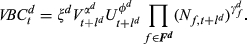

V B C t d = ξ d V t + l d α d U t + l d ϕ d ∏ f ∈ F d ( N f , t + l d ) γ f d .

(1)

The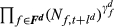

∏ f ∈ F d ( N f , t + l d ) γ f d

term captures the complexity offered, by accounting for the number of options for each feature on the price list, and the

U t + l d ϕ d

term accounts for the complexity built.

We log‐transform this function to use linear regression analysis to estimate needed parameters:

L o g [ V B C t d ] = L o g [ ξ d ] + α d L o g [ V t + l d ] + ϕ d L o g [ U t + l d ] + ∑ f ∈ F d γ f d L o g [ N f , t + l d ] + ϵ t .

(2)

Within our optimization model, we evaluate the effect of a one‐time change to the product portfolio on the long‐term cost. Hence we do not need the time dimension for further analysis and will suppress time subscript t, using a functional representation VBC ^d ( N ^d , V, U) instead. ¹

Estimation of ABC

Introducing a complex option may have different effects: (1) There may be a fixed cost associated with offering the option (e.g., part design cost); and (2) There may be variable costs incurred each time the option is produced (e.g., additional testing each time the part is installed). We model the total cost of offering and producing option o, ABC _o , as the sum of the one‐time cost across all departments if option o is offered (complexity offered) and the incremental cost across all departments incurred each time a configuration with option o is built (complexity built):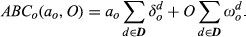

A B C o ( a o , O ) = a o ∑ d ∈ D δ o d + O ∑ d ∈ D ω o d .

Differential Cost of Complexity Function

To facilitate optimization, instead of computing the total cost of each offering, we build a cost of complexity function that starts with the current line and computes the estimated change in cost as the numbers of features and options change. For the variety‐based component, we take the partial derivatives of VBC ^d ( N ^d , V, U) with respect to all variables, and then combine them into an aggregate differential cost of complexity function.

For example, the change in VBC with the number of options for feature f is:

d V B C d ( N d , V , U ) d N f = γ f d N f ξ d V α d U ϕ d ∏ i ∈ F d N i γ i d = γ f d N f V B C d ( N d , V , U ) ,

substituting the definition of VBC ^d ( N ^d , V, U) given by Equation 1.

This differential cost of complexity function includes the predicted value of VBC ^d ( N ^d , V, U). This is problematic for two reasons: (i) The predicted VBC ^d ( N ^d , V, U) contains an error term and hence may not give an accurate size of the cost pool; and (ii) Values of V, N _f , and U change during the specified time period. Therefore, we approximate VBC ^d ( N ^d , V, U) with the historical average cost at department d (

D d ¯

) attributable to complexity, taken over an appropriate period:

d V B C d ( N d , V , U ) d N f ≈ γ f d N f D d ¯ .

(3)

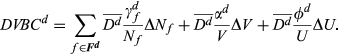
Using Equation 3, the total change in cost of complexity due to a change in the number of options offered for feature f is then estimated as:

D d ¯ γ f d N f Δ N f ,

where ΔN _f represents the change in the number of options in feature f after optimization; similarly we will precede V, U, O, N , N ^d , and V with Δ to represent change. These differential quantities depend on the market response to the options offered in the product portfolio, and will be computed within the optimization model by leveraging our customer migration model. We will formally define these functions in section 5 when we introduce the optimization model.

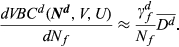
In an analogous fashion, we differentiate the cost of complexity function with respect to volume and number of unique configurations. Aggregating these differences yields the total variety‐based differential cost of complexityDVBC ^d :

D V B C d = ∑ f ∈ F d D d ¯ γ f d N f Δ N f + D d ¯ α d V Δ V + D d ¯ ϕ d U Δ U .

(4)

To capture the differential ABC effect, we must account for the change in the number of options offered and sold. If we eliminate an option o from the price list the cost of complexity will decrease by

δ o = ∑ d ∈ D δ o d

and if sales with option o deviate from O, the cost will likewise change:

D A B C = ∑ o ∈ O δ o ( a o − 1 ) + ∑ o ∈ O ω o Δ O , where a = { a o : o ∈ O } .

(5)

Finally, the total differential cost of complexity is: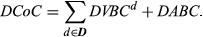

D C o C = ∑ d ∈ D D V B C d + D A B C .

(6)

Equation 6, with estimated parameters, becomes a part of the objective function in the optimization model of section 5. Because the cost of complexity function is non‐linear, this approach is accurate only for small changes. In practice, the accuracy of this approximation may be tested by calculating the actual change in the total cost of complexity for the original product line VBC ^d ( N ^d , V, U) and for the optimized product line VBC ^d ( N ^d  + Δ N ^d , V + ΔV, U + ΔU), and then comparing this to the result of the approximation DVBC ^d .

The Optimization Model

With the migration lists from section 3 and Equation 6 from section 4, we are now ready to describe our optimization model. We use a mixed‐integer linear program to select the set of options and configurations offered, and their prices, to maximize total profit from sales minus the change in cost of complexity (the objective function value increases when this change is negative).

In addition to the data defined in section 4, our optimization model uses the following data:

I — The set of all customers;

L _i — The ordered set of configurations in the migration list of customer i ∈  I . Each member of L _i is represented by a pair (j, k), where k identifies the lane choice and j identifies the specific options chosen for all remaining features. Therefore, the same j can appear in several pairs with different values of k, but only one (j, k) pair will appear in the final portfolio.

J — The set of all configurations appearing on migration lists (

J = ⋃ i ∈ I L i

);

O _jk — The set of all options in configuration (j, k) ∈  J ;

R _i — Reservation price of customer i ∈  I ; this could be configuration‐dependent if desired (i.e., R _ijk instead of R _i );

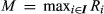
M — Maximum reservation price over all customers (

M = max i ∈ I R i

);

C _jk , B _jk , P _jk — Cost, base price, and current sale price of configuration (j, k) ∈  J , respectively. Base price is the starting price of an incomplete configuration before any of its options are included. The value of P _jk equals of B _jk plus the prices of all options contained in configuration (j, k). We use this additive price structure to illustrate option pricing optimization, but it is not a requirement of our model, that is, other price structures are also possible.

The decision variables (a _o was defined in Table 1, but we repeat it here for completeness):

a _o  = 1 if option o ∈  O is available, 0 otherwise.

q _jk  = 1 if configuration (j, k) ∈  J is bought by at least one customer, 0 otherwise;

x _ijk  = 1 if customer i buys configuration (j, k), 0 otherwise (i ∈  I ,

( j , k ) ∈ L i

);

p _o — Price of option o ∈  O (p _o  ≥ δ _o , where δ _o is defined in Table 1). These variables enable changing the prices of individual options; one could eliminate these variables entirely, or replace them with variables p _jk to price configurations. Using p _jk instead of p _o would result in simple changes to some of the constraints we present below;

r _ijk — Profit if customer i purchases configuration (j,k) (i ∈  I ,

( j , k ) ∈ L i

).

We now provide precise definitions to the following terms that appear in Equation 4 and Equation 5: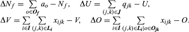

Δ N f = ∑ o ∈ O f a o − N f , Δ U = ∑ ( j , k ) ∈ J q j k − U , Δ V = ∑ i ∈ I ∑ ( j , k ) ∈ L i x i j k − V , Δ O = ∑ i ∈ I ∑ ( j , k ) ∈ L i | o ∈ O j k x i j k − O .

Our optimization model is then: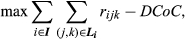

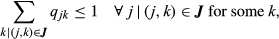
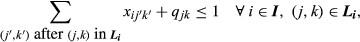
max ∑ i ∈ I ∑ ( j , k ) ∈ L i r i j k − D C o C ,

(7)

q j k ≤ a o ∀ ( j , k ) ∈ J , o ∈ O j k ,

(8)

x i j k ≤ q j k ∀ i ∈ I , ( j , k ) ∈ L i ,

(9)

∑ k | ( j , k ) ∈ J q j k ≤ 1 ∀ j | ( j , k ) ∈ J for some k ,

(10)

∑ ( j ′ , k ′ ) after ( j , k ) in L i x i j ′ k ′ + q j k ≤ 1 ∀ i ∈ I , ( j , k ) ∈ L i ,

(11)

r i j k ≤ B j k + ∑ o ∈ O j k p o − C j k ∀ i ∈ I , ( j , k ) ∈ L i ,

(12)

B j k + ∑ o ∈ O j k p o ≤ P j k ( 1 + m a x _ i n c ) ∀ ( j , k ) ∈ J ,

(13)

r i j k ≤ ( min { R i , P j k ( 1 + m a x _ i n c ) } − C j k ) x i j k ∀ i ∈ I , ( j , k ) ∈ L i ,

(14)

B j k + ∑ o ∈ O j k p o ≤ R i + ( P j k ( 1 + m a x _ i n c ) − R i ) ( 1 − x i j k ) ∀ i ∈ I , ( j , k ) ∈ L i .

(15)

The objective function Equation 7 maximizes the total profit from sales minus the differential cost of complexity given by Equation 6. The purpose of each constraint is as follows (where max_inc is the maximum allowed percentage price increase for any configuration): Equation 8: If option o is not available (a _o  = 0), no configuration that contains o can be bought (q _jk  = 0); Equation 9: If customer i buys configuration (j, k) (x _ijk  = 1), then (j, k) must have been bought (q _jk  = 1); Equation 10: Configurations can be assigned to at most one lane; Equation 11: If (j, k) is bought by someone (q _jk  = 1), it must be available, therefore customer i cannot buy less desirable configurations (j′, k′) that appear after (j, k) in L _i (all

x i j ′ k ′ = 0

); Equation 12: Profit cannot exceed price (

B j k + ∑ o ∈ O j k p o

) minus cost; Equation 13: Configuration prices cannot increase by more than max_inc; Equation 14: No purchase (x _ijk  = 0) means no profit (r _ijk  = 0) and, if a purchase happens (x _ijk  = 1), the term in parenthesis is a ceiling on the value of r _ijk ; Equation 15: If customer i buys configuration (j, k) (x _ijk  = 1), (j, k)'s price must not exceed R _i .

We can turn off the price optimization aspect of this model by removing variables p _o and constraints Equations (13)-(15), and changing the right‐hand side of Equation 12 to (P _jk  − C _jk )x _ijk . Lane assignment decisions can be removed by deleting constraint Equation 10 and all occurrences of index k.

CAT‐Specific Modeling Details

In this section, we first provide some background on CAT's BHL product families, in 6.1. We then detail the assumptions and decisions made to create the CAT‐specific instantiation of the generic framework we describe in sections 3, 4, and 5, (in Sections 6.2, 6.3 and 6.4, respectively). CAT experts participated in the entire process, making sure they understood and, when necessary, validated, the inputs and outputs of each intermediate step.

BHL Product Families

Our product line simplification effort at CAT involved four models in the backhoe loader (BHL) family: 416E, 420E, 430E, and 450E. The 416E is their basic model, while the 420E, 430E and 450E provide progressively superior horsepower and capabilities. We refer to a complete machine as a configuration. Each configuration is composed of features; for each feature, a configuration specifies one of the options within that feature. For example, the feature stick has the options standard and electronic. In the marketing literature, what we call a feature is also known as an attribute, and what we call on option is also known as an attribute level. Table 2 summarizes the features and number of corresponding options present in each BHL model in our project. A dash “‐” indicates that a feature is not present in a model or was not included in our analysis.

OPEN IN VIEWER

Table 2

Number of Options in Each Feature of CAT's BHL Models

Features	BHL models
	416E	420E	430E	450E
Sticks	2	2	2	2
Backhoe hydraulics	3	3	3	6
Backhoe controls	2	–	–	–
Loader buckets	5	13	13	4
Loader hydraulics	2	2	2	2
Cab/canopy	5	5	4	2
Powertrain	4	3	2	–
Engine cooling	2	2	2	–
Counterweights	4	4	4	–
Backhoe aux lines	3	3	3	3
Engine coolant heater	1	1	1	1
Product link	1	1	1	1
Ride control	1	1	1	–
Front loader mechanics	–	2	2	–

To create a complete configuration, a customer selects one option for each of its features, ensuring that these options are compatible. The number of such configurations is immensely large: For model 416E in its most basic version, there are 37,920 feasible configurations. Including choices for attachments yields 2,275,200 distinct feasible configurations. The vast majority of these configurations have never been, and most likely will never be, built. The mere fact that they could be purchased, however, creates overhead costs for CAT. Moreover, every unique option offered incurs a cost for CAT, due to the engineering and support costs it requires. We discuss this in detail in section 4.

So how many configurations are actually built? Figure 1 depicts the minimum number of different configurations (left panel) and options (right panel) required to capture given percentages of revenue and sales, respectively, for eight month's worth of sales data for model 420E. Of the 569 built configurations, 400 were needed to capture about 95% of revenues and sales volume. Similarly, 36 out of the 42 available options were needed to capture at least 95% of revenues and sales volume. Therefore, to achieve the sought reductions in product offerings, it was imperative to steer purchases toward a considerably smaller subset of products and options.

OPEN IN VIEWER

Figure 1

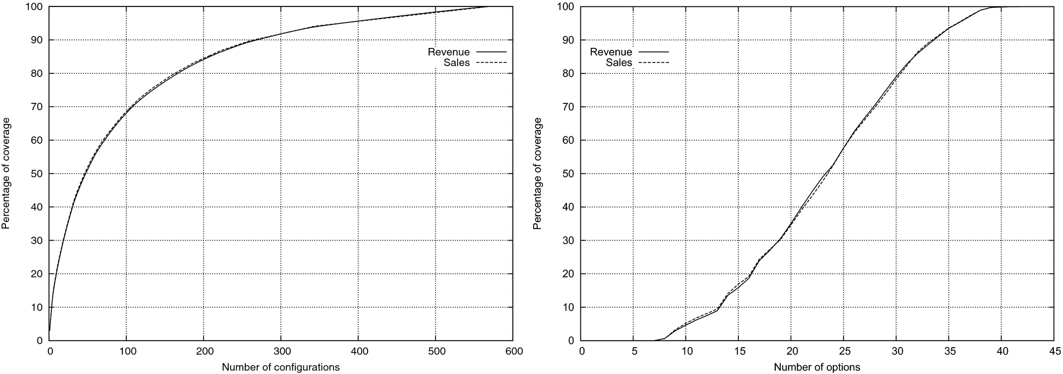
Minimum Number of Distinct Configurations (Left) and Options (Right) Required to Capture Given Percentages of Revenue and Sales Volume for BHL Model 420E

As we will see in section 8, CAT ultimately converged on a lane system in which configuration lead times depend on the lane to which they belong. Although not part of our original algorithm, our modeling framework can incorporate such a structure assuming the lanes and lead times are given. Specifically, lanes, with corresponding lead times, can be treated as options of an additional configuration feature, which we will call Availability. In addition, just as customers can be modeled as having tolerances for price and utility, there can be a maximum availability threshold per customer as well.

Modeling the Behavior of CAT's Customers

The pseudo‐code below shows how migration lists were constructed for CAT; we use customer purchases in 2006 as the basis for generating our migration lists.

For each customer i ∈  I who bought a configuration over the past H months repeat:

Let M _i be the configuration (i.e., machine) bought by i.

Apply segmentation rules to M _i (section 6.2.1) to place i in a customer segment S _i .

Based on the price and utility of M _i , and on characteristics of segment S _i , construct a randomized list of configurations, L _i , as acceptable alternatives to M _i (section 6.2.2).

Sort L _i in non‐increasing order of configuration utility, pruning it if it exceeds the maximum allowed length (section 6.2.3).

Customer Segmentation

Customer segmentation is important in CAT's business because it affects customer flexibility. For example, customers who live in extreme weather conditions are unlikely to buy a configuration that does not include a cab with climate control, and customers who need to carry very heavy loads are not willing to sacrifice horsepower. We used focus groups composed of CAT experts and actual customers to identify the main customer segments and their characteristics: performance extreme (PE), performance extreme versatility (PEV), performance mild (PM), performance mild versatility (PMV), commodity extreme (CE), and commodity mild (CM). The performance category represents customers who are less price sensitive and need powerful machines. The extreme and mild categories refer to weather conditions, and the versatility category represents customers who need their machines to perform a variety of tasks. Based on historical sales data, the fraction of customers in each of the above six segments are approximately 20%, 20%, 25%, 10%, 5%, and 20%.

A set of segmentation rules was created to classify each purchase: Given a configuration, its customer segment is determined by the presence and/or absence of certain options, represented as part numbers. For example, there are eight ways for a 416E loader to be placed in segment PE. One is: Two out of the options 2,146,913, 2,099,929, and 2,139,293 must be present (89HP powertrain and e‐stick), and one out of the options 2,044,161, 2,044,162, and 2,284,602 must be present (cabs), and the option 2,120,206 cannot be present (6‐function hydraulics), and neither option 2,497,912, nor option 2,624,213 can be present (one‐way and combined auxiliary lines).

In addition to the segment‐specific option utilities discussed in section 6.2.2, segment‐specific reservation prices and reservation utilities also affect migration list generation (section 6.2.3).

Estimating Utilities

For each of the customer segments identified in section 6.2.1, we calculate option utilities as follows. First, to estimate the importance of a model's features, we asked a group of CAT employees with sales and manufacturing expertise to use the Analytic Hierarchy Process (AHP) (Saaty 1980). AHP asks experts to estimate the relative importance between every pair of features on a scale from 1 (equally important) to 9 (much more important). The pairwise scores are then transformed into absolute scores of relative importance for each individual feature. The same group of experts is then asked to rank the options within each feature on a scale from 0 to 100. These option scores are scaled so that the option receiving a score of 100 is assigned a value equal to its feature's relative importance. These scaled scores represent the final option utilities. The utility of a complete configuration is estimated as the sum of the utilities of its options.

To validate the utility values calculated for each of the options—for every BHL model in all customer segments—we conducted a survey asking actual customers to choose among alternate configurations. Using t‐tests, CAT determined that differences between the utilities derived from the survey results and those estimated by experts were not statistically significant.

Building Migration Lists

Although customers of a given segment tend to behave similarly, they are certainly not identical. To account for variations within each segment, we modify the migration list procedure in several ways. First, for each segment we randomly perturb the relative importance (and, consequently, the option utilities) of randomly selected features. The number of features to perturb is an input parameter (for CAT, this was around three). Given a perturbation factor θ (approximately ten), the change to a feature's relative importance is randomly drawn from a uniform distribution over the interval [−θ%, + θ%]. CAT also did not want customers to have lists containing configurations too dissimilar from the one purchased. Therefore, a number called the disparity factor (around five) limits how many options an alternative configuration can have that differ from M _i . Finally, the model generates the customer's reservation price and reservation utility; again, these values are randomly picked from a predetermined interval around the price and utility of M _i . ²

We collect the above procedures into a Constraint Programming (CP) model (Marriott and Stuckey 1998) that finds feasible configurations for L _i . This CP model needs to know what constitutes a feasible configuration, that is, which options are compatible. We use configuration rules to describe these interdependences. For example, for model 420E, one rule is: If a configuration has option 9R58666 and either option 2139272 or 2139273, then it cannot have option 9R5321. After all feasible configurations are found, those that exceed the generated reservation price or fall short of the reservation utility are pruned from the customer's migration list.

Next, configurations are sorted in non‐increasing order of total utility and L _i is truncated, if desired, while respecting two conditions. First, if L _i is truncated, M _i must always be retained. Second, we assume customers place M _i first, regardless of M _i 's utility, with a certain probability (the β factor; for CAT it was between 0.3 and 0.7). This is an attempt to capture the fact that some customers are attracted to their M _i for reasons we cannot capture with utilities.

Migration across different models is also possible. In this case, we apply a set of migration rules that map a purchased configuration M ₁ of model m ₁ (e.g., 416E) to its most likely counterpart M ₂, of a different model m ₂ (e.g., 420E). Once M ₂ is known, we generate alternatives as if it were the customer's original purchase, and include them (together with alternatives to M ₁) onto L _i . Because m ₂ configurations may have higher utilities, when L _i is sorted it may contain almost no highly ranked m ₁ configurations. Thus, to capture the fact that customer i originally preferred an m ₁ configuration, we inflate the utilities of all m ₁ configurations on L _i by a preference factor (between 10% and 20%). As a result, L _i ends up with configurations of both models, but it does not allow utilities to overemphasize the attractiveness of m ₂ configurations. According to CAT, the plausible model migrations are from 416E to 420E and from 430E to 420E.

As was done for option utilities, we also conducted an extensive validation study with CAT experts to evaluate the quality of our migration lists. Throughout this process, the experts provided valuable feedback that helped us fine tune our input parameters. After a few iterations, CAT experts agreed that our migration lists could be safely used by our optimization algorithm.

Estimating the Cost of Complexity at CAT

Understanding the Impact of Complexity at CAT

In conjunction with CAT experts, we identified nine functional areas impacted the most by complexity. Within each area, we (i) identified up to three major processes most impacted by product complexity; (ii) found cost‐measures that capture the impact of complexity for each major process; and (iii) identified particular product features and/or options that have the largest impact on the cost of complexity. Table 3 lists the functional areas, processes impacted, and measures used (when alternate cost measures are used due to data unavailability they are denoted by a dagger †). Below, we elaborate on several cost measures in Table 3.

OPEN IN VIEWER

Table 3

Main Business Processes Impacted by Complexity and the Corresponding Cost Measures

Department	Processes impacted	Measure of complexity
Purchasing	Capital tooling	Capital tooling cost
	Supplier operations	Supplier delivery performance 1
Customer acquisition	Ordering
	Forecasting	Cost of customer acquisition 1
	Quoting and training
Marketing	Price list creation
	Training	Budget expenditure 1
	Publications
Engineering	Drawing changes	Cost of engineering changes
		Cost of product and component
	Original design and development	Cost of new releases
Order fulfillment	Attachment forecasting
	Sequencer work	Headcount cost 1
	Grief resolution
Product support	Dealer solution network ‐ calls	Cost of service calls
	Publications ‐ manuals	Cost of publications
	Warranty costs	Cost of repairs (first 10 hours)
		Cost of repairs (during 11–100 hours)
		Cost of repairs (above 101 hours)
Material planning	Inventory management	Inventory handling cost (prime product)
		Inventory handling cost (components)
	Schedule volatility	Headcount cost
	Expedition	Freight cost
Operations	Initial process setup	Person‐hour cost, production planning
	Assembly process	Person‐hour cost, assembly
Quality	Initial setup	Cost of initial setup
	Hot test	Hot‐test cost (person‐hours)
	Cab test	Cab‐test cost (person‐hours)

Note

Alternative cost measures used due to lack of data availability.

Cost of supplier delivery performance refers to a program targeted towards improving availability, in which CAT contacts suppliers with low delivery performance to improve their processes. We use the cost allocated to this program as a proxy for the cost of supplier operations. In the customer acquisition department, CAT calculates sales variance cost by tracking all the discounts that go into making a sale: invoice, extended service, cost of free attachments, etc. We use this measure to approximate the cost of customer acquisition. We rely on CAT's accounting system for cost estimates of engineering changes (primarily consisting of payroll to engineers working on changes) and engineering of new releases (primarily consisting of the payroll of developers and engineers who work on new parts, and costs of testing and design equipment).

Option Effects for CAT

The next step was to understand which features have VBC and/or ABC effects on identified processes. The results of VBC/ABC classification are summarized in Table 4.

OPEN IN VIEWER

Table 4

VBC/ABC Classification of Features

Department/feature	Backhoe hydraulics	Loader buckets	Auxiliary lines	Quick coupler	Hoe buckets	Control groups	Cab/canopy	Sticks
Purchasing		VBC		VBC	VBC		VBC	VBC
Customer acquisition	VBC		VBC				VBC
Marketing	VBC		VBC				VBC
Engineering	ABC	VBC	VBC		VBC		ABC
Order fulfillment	VBC	VBC	VBC	VBC	VBC	VBC	VBC	VBC
Product support	VBC		VBC				VBC
Material planning	VBC	VBC			VBC		VBC
Operations			ABC				ABC	ABC
Quality							ABC

Temporal Effects for CAT

We then estimated the time lags for different cost pools, some time lags are naturally incorporated into the cost data based on the accounting rules, but some needed adjustments. Table 5 summarizes our analysis of time lag parameters. We use this information in section 6.3.5 to estimate the parameters of the cost of complexity function.

OPEN IN VIEWER

Table 5

Summary of the Time Lags (in Months)

Department	Time lag	Department	Time lag
Purchasing	0	Product support:
Customer acquisition	3	Service calls	6
Marketing	0	Repairs in the first 10 hours	4
Engineering:		Repairs in 10–100 hours	9
Changes	−6	Repairs after 100 hours	9
Releases	−8	Material planning:
Product and component costing	−7	Prime product inventory	2
Order fulfillment	0	Scrap of surplus materials	0
Operations	0	Inventory scrap	0
Quality	0

Volume Effects for CAT

Similar to the time lags, we collected initial estimates of the primary volume drivers for different cost pools from the experts in each department, summarized the results, and held a group discussion to come to consensus. Table 6 provides a summary of the results.

OPEN IN VIEWER

Table 6

Main Volume Drivers

Department/volume driver	Sales volume	Complexity offered	Complexity built
Purchasing	✓		✓
Customer acquisition	✓	✓
Marketing	✓	✓
Engineering		✓
Order fulfillment	✓		✓
Product support	✓		✓
Material planning	✓	✓	✓
Operations	✓		✓
Quality	✓		✓

Estimation of the VBC Effect

With a good understanding of the costs, time lags, and volume drivers, we collected data to estimate parameters ξ ^d ,

α d

,

ϕ d

, and

γ f d

for all d and f. We collected data from January 2001 to December 2005, for all cost measures summarized in the third column of Table 3. We then collected data from the price lists from 2000 to 2006 to capture all changes in option offerings, which were used as independent variables. (We had to collect a larger range of data due to the time lags identified in section 6.3.3.) Similarly, we collected monthly sales (V _t ) and the number of unique configurations sold per month (U _t ) from 2000 to 2006.

The nature of the data suggested that there may be serial correlation, hence, we examined partial autocorrelation function plots and checked for autocorrelation, using the generalized Durbin–Watson statistics using the AUTOREG procedure in SAS. For those cost pools having autocorrelation (all three “Cost of repairs” measures), we used the autocorrelation order identified by SAS (all three were a lag of one) and used the Yule‐Walker approach to fit the data (Greene 2000).

Next, we obtained statistical models for all departments by fitting collected data to Equation 2. We evaluated our models using both graphical and numerical tests using standard statistical techniques (e.g., examined the plots of residuals for normality, heteroscedasticity, and influential outliers). Although our cost data exhibited seasonality, the seasonality in cost (our dependent variable) is driven mainly by the seasonality in the volume (an independent variable) and, hence, it is likely to be automatically taken into account by our model. We checked this by analyzing residuals: In each model, we group the residuals for each month; F‐tests show that there are no statistically significant differences between the means of the groups. We also checked for significance, and only accepted those factors with reasonable coefficients of determination and low RMSE. Hence, not all of the originally identified departments were included in the final cost of complexity function. Table 7 summarizes all models/departments included in the optimization model. The estimates that are statistically significant at the 0.05 significance level are marked with an asterisk. ³

OPEN IN VIEWER

Table 7

Fit Results

Fn.	Cost pool (d)	R 2	RMSE	ξ d	α d	ϕ d	γ H C d	γ C d	γ C W d	γ H d
CA	Customer acquisition	0.37	0.18	962,771,120.4 1	0.19			−1.13 1		−1.68 1
MP	Inventory (components)	0.29	0.16	1,087,617.41 1	−0.03			1.04 1
MP	Inventory (prime product)	0.38	0.4	297.68	0.91 1	0.91
ENG	Engineering changes	0.41	0.52	0.00342591			4.81712 1	−0.54
ENG	Engineering product and component	0.55	0.9	6.39E‐04 1			4.107 1		3.14 1
PS	Repair costs in the first 10 hours	0.29	0.37	26,238.94 1	−0.21	0.59 1
PS	Repair costs during 11–100 hours	0.32	0.24	3055.00 1	−0.32	1.28 1
PS	Repair costs above 101 hours	0.55	0.47	934.63 1	−1.41 1	2.78 1
P	Supplier delivery performance	0.33	0.58	36.65		1.5 1

Notes

Statistically significant parameters at 0.05 significance level. Subscripts HC, C, CW and H stand for hydraulic combinations, cabs, counterweights, and hydraulics.

We comment on the coefficient of determination (R ²) of the models in Table 7. Some of the departmental costs are heavily impacted by factors outside CAT's walls: For example, cost of customer acquisition is impacted by competitors’ actions, and cost of supplier delivery performance is impacted by suppliers’ operations. Hence, we expect the coefficients of determination to be lower for such departments. In running the optimization model, nevertheless, in order to help ensure that our results are robust, we evaluate ranges of parameters as described in section 7.

Some other findings in Table 7 are noteworthy. Increasing the number of options for hydraulics and cabs decreases the cost of customer acquisition, that is,

γ H C A < 0

and

γ C C A < 0

: A large proportion of this cost consists of sales variance or discounts given to customers in order to attract business. Cabs and hydraulics are very important considerations for customers; having a large selection of options for these features makes it easier to make a sale, decreasing the sales variance. This finding is in line with the intuition of sales and marketing representatives from CAT. Nevertheless, this was the first time that CAT was able to quantify this effect.

Another observation is that sales volume has a negative impact on product support costs (i.e., repair costs): When volume goes up, CAT employees assemble more machines with the same options, and learning effects reduce the number of mistakes. This intuition again seemed plausible to CAT, but had never been quantified. On the other hand, sales volume has a positive impact on the cost of inventory of prime product. As CAT subsidizes dealers for carrying final product inventory for time sensitive customers, and the lead time demand increases when volume increases, subsidies increase. Guided by our study, CAT subsequently has performed similar cost of complexity analyses in other product divisions and obtained comparable results.

Finally, we validated our model by using the first two years of data to fit the model, then, compared the predicted values for the next three years to actual data. A large majority (7 out of 9) of the actual cost pool values were within the 95% confidence interval around their predictions.

Estimation of the ABC Effect

From focus groups, we identified that ABC effects were observed primarily in three departments: assembly, production planning, and engineering. The nature of work in these departments suggested a linear relationship between ABC cost and complexity: If it takes 5 extra minutes to install a particular option on a machine, this cost will apply to each machine that contains the option. This coincided with expert opinion, which posited minimal learning effects. This supported the form of our proposed ABC _o function having a fixed and variable cost component.

The cost parameters δ _o and ω _o were estimated using expert opinions, time studies, and accounting information from all functional areas that identified this option as important (see Table 8).

OPEN IN VIEWER

Table 8

ABC Costs

Option	δ o	ω o
Any option	$1000.00
In addition
IT	$6000.00	$23.61
Cab	$14,656.25	$53.80
E‐Stick	$125.00	$1.30
One way line	$3593.75	$5.64
Ride control	$1281.25	$5.86

CAT's Optimization Model

CAT used the optimization model in section 5 without its lane‐assignment features. In addition to the constraints described therein, CAT's optimization model includes two constraints that deal with profit margins. Let 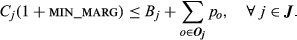min_marg and min_avgmarg be, respectively, the minimum required profit margin on each configuration sold, and the minimum required average margin over all configurations sold. The margin constraint per configuration is written as

C j ( 1 + m i n _ m a r g ) ≤ B j + ∑ o ∈ O j p o , ∀ j ∈ J .

(16)

CAT provided a specific formula that they use to enforce the minimum average margin over all configurations sold. Besides the configuration cost C _j defined in section 5, CAT uses another cost figure, denoted

C j ′ ≤ C j

, which they refer to as variable cost. The sole purpose of

C j ′

is to enforce this average margin constraint: ⁴

m i n _ a v g m a r g ∑ i ∈ I ∑ j ∈ L i ( r i j + C j q j ) ≤ ∑ i ∈ I ∑ j ∈ L i ( r i j + ( C j − C j ′ ) q j ) .

(17)

The resulting optimization models have around 850,000 variables and 1.8 million constraints, they are solved, using ILOG CPLEX Optimizer with default parameters. Typical solution times range from 6 to 8 hours, including preprocessing.

Results from Our Analysis

CAT's goal was to make a drastic reduction in the number of configurations offered without significantly reducing customer satisfaction or market share. How to achieve such a goal, or whether it was even possible, was unclear at the outset of the project. Since this reduction would present customers with fewer configurations, CAT assumed each remaining configuration could be priced a little lower; the reduced cost of complexity would allow this while maintaining profit.

Throughout our analysis, to ensure that our recommendations were robust, we ran the optimization model across a range of parameters and migration list lengths.

Stage 1: Focusing on Configuration and Option Reduction

As an initial benchmark for our optimization, we first sought to identify the set of configurations that maximized profit at the current option prices, assuming limited customer migration (no more than a dozen configurations on a migration list, and no migration across models). While profits did increase, we obtained very little reduction in the number of configurations, except when a reduction was explicitly enforced by the constraint

∑ j ∈ J q j ≤ ( 1 − m i n _ c o n f _ r e d ) | J |

. Moreover, forcing a large reduction resulted in a significant decrease of sales revenue.

Given these results, we hypothesized that further reducing the cost of complexity would require significant cuts in options. Hence, a new constraint was added to the model to force option reduction:

∑ o ∈ O a o ≤ ( 1 − m i n _ o p t _ r e d ) | O |

. We re‐ran the optimization model forcing a reduction in the number of configurations and the number of options. Reducing options did succeed in reducing configurations, in some solutions by as much as 94%, and increased profit by generating a large cost of complexity reduction. But it also resulted in a drop in sales volume of up to 67%. This disturbed CAT team members since the company has always prided itself on its market share. Fulfilling customer demand therefore became an important new metric of the analysis.

Stage 2: Opening Up Choices

Thus, in the next phase of our analysis, we wanted to explore what results would be possible if customers were presumed to be significantly more flexible, possibly as a result of price incentives. We modeled this flexibility in two ways: We increased the migration list length (to 100 configurations) and we enabled model‐to‐model migration.

This approach started to generate encouraging results. A solution emerged with an increase in profit of 8.8%, less than a 2% reduction in sales volume, and a reduction in configurations equal to 65%. But further analysis showed that the number of options had not decreased significantly. The increase in profit came from a decrease in the number of configurations, and increases in price paid by customers who migrated to slightly more expensive machines. Performing sensitivity analysis confirmed this conclusion: Expecting a large reduction in options was not realistic. However, a large reduction in configurations was possible.

This resulted in a problem for CAT: Without a reduction of options, how would this new (and limited) set of configurations be presented to the customers? Restaurants can get by with a 3–4 page menu that lists all their entrees. But no customer would flip through a menu of 70–90 pages listing all the possible BHL configurations. A new scheme had to be devised.

Stage 3: Standardization and Options Packages

We decided to try two new strategies to concentrate customer demand on a manageable number of configurations. The first strategy was standardization: Could options such as High Ambient Cooler and Engine Heater be made standard across all configurations? Optimization models with these options forced into every configuration yielded cost reductions that justified a reduction in price large enough to make the standardized configurations attractive to customers, while maintaining sales volumes and profit. Other rarely used options were eliminated, using a similar approach. For example, the Cab/Canopy options were cut from five to two.

The second strategy was creating packages of options commonly found together. For example, guided by customer segment preferences, a single pair of loader hydraulics and powertrain options most likely to meet each segment's needs were proposed. Manual inspection and cluster analysis of the best solutions found so far led to the discovery of other options often found together.

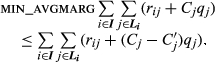
The optimization was then run assuming standardization and option packaging, with constraints on the maximum price increase. This yielded the final product hierarchy for the 420E series, shown in Figure 2: It consists of 9 base‐machine‐assembly (BMA) packages, 5 finished‐to‐order (FTO) packages, and 3 hydraulics options, for a total of 135 possible configurations, some of them anticipated to be much more popular than others.

OPEN IN VIEWER

Figure 2

Final Product Hierarchy and Packages for the BHL 420E Series

Pricing optimization showed that with these 135 configurations, revenue from sales could increase by almost 7%, and profit could increase by 15%, with 99.6% demand fulfillment. The standardization and bundling of options greatly reduced the universe of feasible configurations, which led to inventory and quality savings: 76% of the projected cost of complexity savings came from reductions in finished goods inventory and warranty costs (in particular, the cost of addressing failures in the first 100 hours of machine operation). Since the goal of the project was to maintain similar profit levels (rather than seeking increases), the team determined appropriate option price reductions to drive dealer behavior toward these configurations while maintaining profit. The proposed pricing policy resulted in an anticipated reduction in profit from sales of 4%, which was easily made up by the reduction in cost of complexity to yield a total profit increase of 4.8%. We had finally found the very small subset of configurations that we believed was broad enough to satisfy CAT's customers and dealers, but also focused enough to drive operational and supply chain efficiencies. This final recommendation was presented to CAT, and was approved.

Implementation Details

Initial Implementation

CAT put an updated price list for the 430E product line (modified via dealer input to now feature 124 configurations) into effect in some regions in April 2010; but, in order to minimize the risk of lost sales, customers could still order a‐la‐carte machines according to the old price list. Concurrent with this new price list, CAT introduced a 3‐lane strategy for order fulfillment:

Lane 1 (the fastest lane): Orders on the four designated “most popular” fully configured machines would be satisfied within a few days;

Lane 2: Orders on the remaining 120 choices, broken into the Loader, Comfort and Convenience, and Excavation packages, would be satisfied within a few weeks;

Lane 3: Any a‐la‐carte machine would be satisfied within a few months, as previously.

Upon implementation, CAT experienced positive dealer feedback and large reductions in the number of unique configurations sold. This contrasted with previous attempts to reduce the size of the product line, based on a Pareto analysis of the top few dealers. These had likely been ineffective, in CAT's opinion, because they did not effectively model the interaction of cost, customer preferences, and substitution, as we had.

It is worth noting that, to the best of our knowledge, neither standardization nor option packaging were being considered prior to the start of our project. These concepts, and the lane strategy they support, were only developed after our analysis indicated that CAT needed to find a way to limit the number of configurations while not eliminating too many options. Our analysis then gave CAT direction in implementing these new strategies, by indicating which sets of configurations were likely to be most successful.

This evolution of the solution strategy also affected how the results of our algorithm were applied. Specifically, we initially modeled a problem setting in which there would be a reduced set of products offered to customers differentiated by price, but not by lead time. The solution CAT implemented (in principle) still includes all possible configurations within Lane 3, and differentiates these from the first two lanes by lead time. Thus, our forecasts of the savings in cost of complexity, which would be accurate if only the first two lanes were offered, are only an approximation given the continued possibility of a‐la‐carte ordering. Caterpillar felt that the flexibility of retaining Lane 3 outweighed any reductions in cost of complexity savings. Likewise, although lead time differences could be incorporated into our framework as shown in sections 3 and 5, Caterpillar felt comfortable enough with the main conclusions of the analysis to forgo additional analysis.

Moving Forward

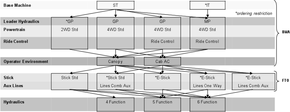
In 2011, CAT released a single price list featuring options packages for use in all regions. They were able to capture over a quarter of their sales volume just in Lane 1; in contrast, the four top‐selling configurations CAT offered before this project captured 11.3% of both sales and total revenue for the 420E model (Figure 1). In addition, CAT enjoyed a reduction in warranty costs, attributable to many factors, including this project. CAT has continued to focus their BHL offerings, for example reducing the 420E (now the 420F) Lane 1 offerings to three base machines by mid 2014. The other BHL lines have seen similar reductions.

The lane approach has become an integral part of CAT's business strategy (Thomson Reuters 2014). While the methodologies used to determine lane offerings in other divisions were somewhat simpler than the analysis done here, our work provided support for the corporate‐wide lane strategy. In particular, our cost of complexity analysis approach has been applied to other divisions, such as Wheel Loaders, with the goal of capturing all the benefits and understanding all the consequences of proposed line changes. The detailed analysis and structured optimization approach reported in this study allowed CAT to counteract skepticism toward the lane approach embarked upon by BCP prior to the diffusion of this strategy throughout the company.

Sensitivity Analysis and Insights

In order to generate additional insights from our model, we conducted an extensive sensitivity analysis of our framework by running a large number of experiments in which we vary the main input parameters over a range of values and record key output measures. Because of space limitations, we do not include all of the experiments here; they are available in a separate Appendix S1 to this article. This section summarizes the main findings generated by this analysis.

Modeling Customer Behavior

Customer Flexibility: The More the Better

As customers become more flexible and willing to accept a wider range of configurations, the expected effects include a decrease in the number of configurations needed to satisfy them, a reduced number of required options, decreased complexity costs, and higher profits. These trends are supported by our experiments; specifically, when any of the following parameters increases in value: maximum migration list length, reservation price, disparity factor, and percentage of novel configurations in the portfolio. Varying the number of features whose utilities are perturbed and/or the amount of perturbation around the point estimate (perturbation factor) seems to add some noise, but does not ultimately change the observed outcomes significantly.

Role and Effect of Migration Lists

While performance improves with longer migration lists, we note that the effects of greater list length is more pronounced for smaller lists—once lists are of moderate size (about forty) metrics are largely insensitive to further increases in length (see Figure 3, additional figures and discussion are provided in Appendix S1, section 1). Furthermore, more choices lead to purchases being more spread through migration lists, decreasing the number of top‐ranked purchases, as these are knocked out of the portfolio in favor of more universally appealing configurations.

OPEN IN VIEWER

Figure 3

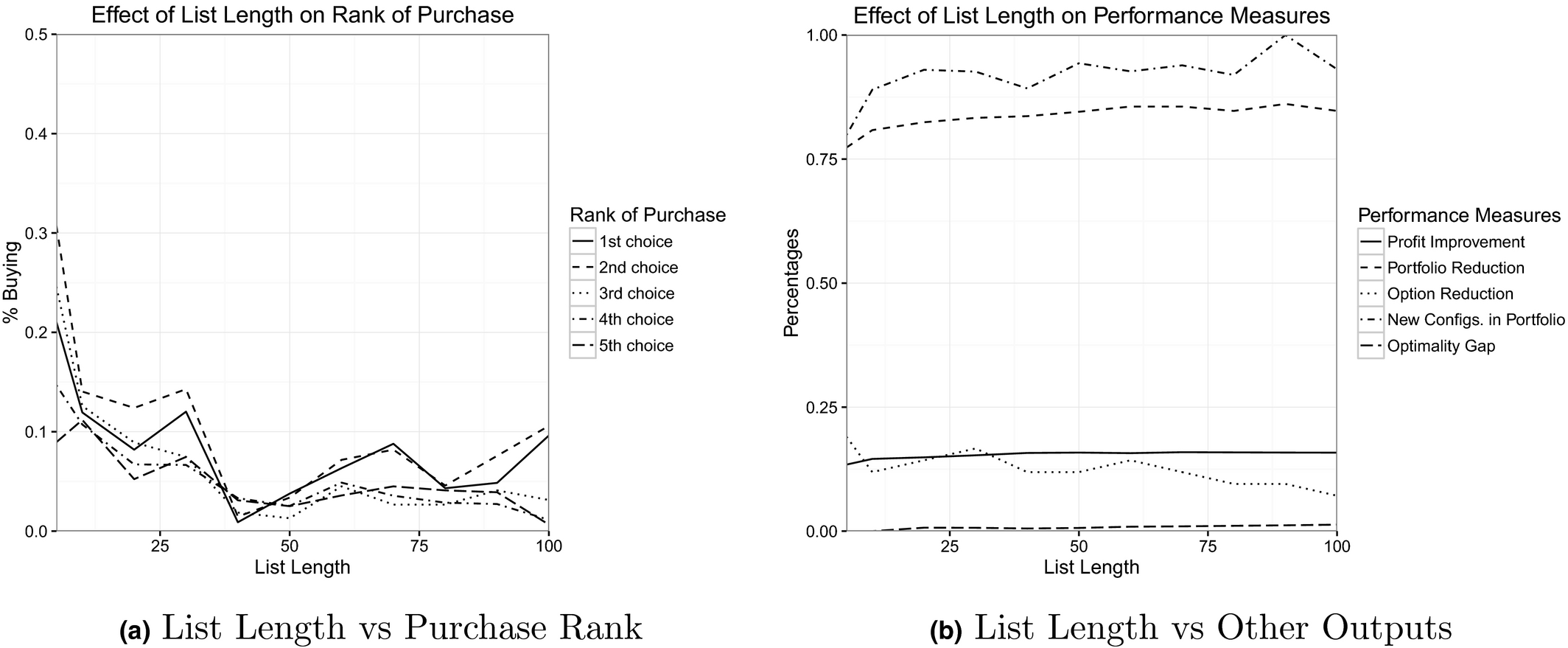
Effect of Migration List Length

To better explain the role of migration lists, Figure 4 shows how many times, out of 3825 customers, a customer's original choice ended up at a given position on that customer's (100 configuration long) migration list (note the log scale on the vertical axis). The rightmost, tallest bar indicates that for 2601 customers (68% of the time) a customer's original choice would not have appeared anywhere in the first 100 positions of the customer's list. For CAT this means that, for over two thirds of their customers, there are many products that provide them with higher utility than the first product they had in mind. Figure 4 emphasizes that, within the context of product portfolio reduction, the main purpose of migration lists is not to predict what a given customer would buy. Rather, the migration list's job is to determine which products would provide high utility to each customer, thus forming a pool of configurations from which to select the ultimate product portfolio.

OPEN IN VIEWER

Figure 4

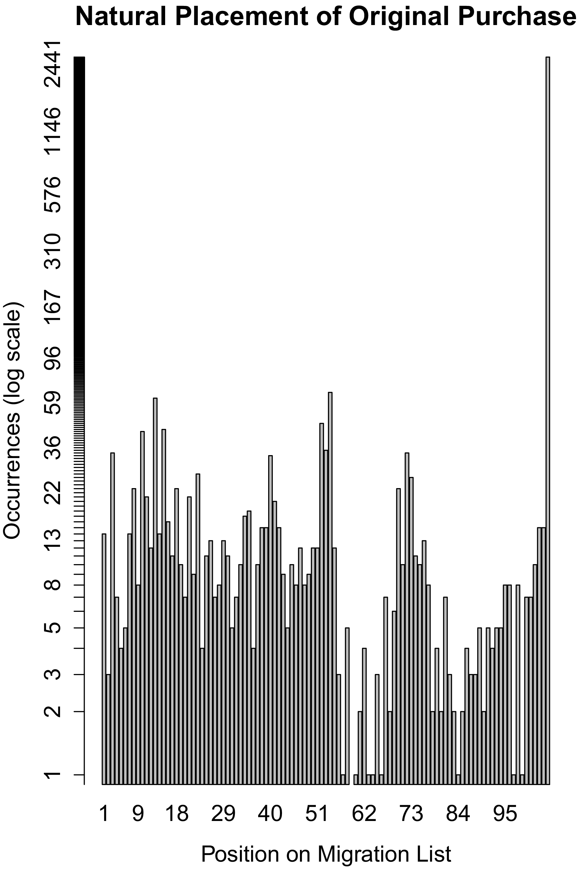
Number of Migration Lists, Out of 3825, Containing Original Purchase

To explore this point further, consider the following thought experiment: Assume a company had a perfect forecasting algorithm that could always guess exactly what any customer's first choice of product would be. Despite being useful for several things (such as targeted advertising, as well as production and inventory planning), if the universe of customers’ first choices were very heterogeneous, this algorithm would not allow the company to reduce the size of its product portfolio because it would not provide any information about customers’ flexibility and willingness to substitute. Instead, a migration list, as defined in our framework, tries to predict, given a customer's first choice of product, what other products would likely be acceptable to that customer. In doing so, if a large number of customers happen to like the same not‐so‐large collection of products, there is a chance that significant savings can be achieved by focusing the portfolio on that smaller collection, even if some of those products are not the first choice of many, or even any, of the original customers.

Varying the β Factor

As β goes up, the probability of buying the first configuration on the migration list goes down. This is likely because many of the originally purchased configurations are pruned from the portfolio in an effort to concentrate customers. As for profit, it is largely insensitive to β, even though the composition of the portfolio may change.

Reservation Price Vs. Reservation Utility

As expected, when customers are willing to pay more, everything improves for the company. Customers whose β factor does not force their originally purchased configuration to appear first on the list are more likely to buy their top choice, as it will likely be a high‐utility, high‐price machine. The remaining customers are more likely to purchase configurations further down their migration lists, as their top, lower utility/lower priced choices get pruned. In contrast, having customers willing to accept lower utility machines is not as impactful as their becoming less price sensitive. That is because accepting machines with lower utility does not remove the higher utility machines from consideration (which the company would typically prefer to sell anyway), and the latter get placed ahead of the lower utility machines on the migration lists.

Role and Effect of the Number of Lanes

The concept of lanes introduced in section 8.1 adds another dimension to a configuration's attractiveness: Availability, that is, how quickly a customer can obtain it. Availability can be treated as a feature whose options are fastest, second fastest, etc. As a feature, availability would then have a relative importance and its options would have utilities. And, given these utilities, the company may choose to either charge a premium/markup for configurations in faster lanes or keep the prices the same. We ran a set of experiments to understand what happens to customers’ migration lists and to several output measures related to the optimal product portfolio when different numbers of lanes are present (e.g., the company decided to offer 3 lanes instead of 2). For the optimization algorithm, what matters are the configurations on each migration list, as well as the order in which they appear. Hence, we simulate the presence of the availability feature by exploring the composition of migration lists under different lane scenarios. One benefit of this approach is that it does not require us to choose exact values for different costs and profits related to different lanes, as would be required to run a full‐blown optimization.

For our experiments, we first need to characterize customers based on two dimensions: willingness‐to‐pay (low, medium, high) and the utility they assign to the availability feature (low, medium, high). Note that these are two different things: A customer may prefer to have high availability, but be unwilling to pay extra for it. As an example of how we categorize customers, consider a case with three lanes where Lane A is the fastest and Lane C is the slowest. A customer who has low willingness‐to‐pay (wtp) and low utility for availability (avail), will only have the slowest lane on his migration list (C), and a customer who has low wtp and medium avail, may have a migration list comprised of configurations in lanes C and then B (CB). For our experiments, we consider 10 different values for the Utility of Availability (specifically, from 1 to 10), such that: a customer with low avail is mapped to value of 1, medium to 5, and high to 10. The values in between capture the gradual transition in the proportion of customers switching to the type of migration list: namely, for customers with low wtp, when the utility of availability equals 1, all customers have only one migration list (C), but as the values increase from 1 to 5, the proportion of customers switching to list CB increases. The exact proportion of customers corresponding to each utility value depends on the selected percentage of customers having different wtp. ⁵ In addition, we consider cases with and without a price markup on faster lanes as some companies may have no markup and use the lanes solely to incentivize customers to purchase certain subsets of products, while others may put a markup on the configurations offered in faster lanes.

In this section, we report the results on the effect of utility of availability for an experiment without price markup, where the customers are split equally between the wtp values. ⁶ We provide additional results from multiple experiments in Appendix S1 in section 2. In Figure 5a, we demonstrate what percentage of profit is attributable to each lane as the utility of availability changes. Notice that as the utility of availability increases, Lane 3 (the slowest lane) gets utilized less and eventually disappears. This observations persists across scenarios with different markups and different distribution of customers across wtp values. In Figure 5b, we compare the profit of five replications of the portfolio with 2 lanes vs. the portfolio with 3 lanes and show that when the utility of availability is low, the 2‐lane portfolio provides a higher profit than a 3‐lane portfolio, but the opposite is true when the utility of availability is greater.

OPEN IN VIEWER

Figure 5

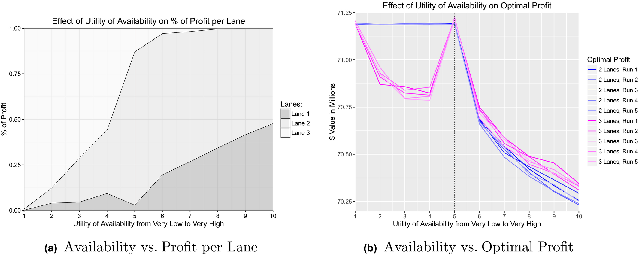
Effect of the Utility of Availability [Color figure can be viewed at wileyonlinelibrary.com]

This arises because the overall portfolio size of the two lane portfolio stays comparatively more stable than the three lane portfolio for smaller utilities – there is just less room for movement. But once availability becomes more valuable, there is greater dispersion among the customer base, and thus the three lane portfolio has an easier time accommodating this: While both portfolios grow, the two lane portfolio grows more abruptly, lowering the profits. ⁷ Note that these experiments were run for the case of zero markup – as expected, when markup is permitted profit increases with the utility of availability, as customers are steered toward more expensive, more available, machines. Note finally, that these effects remain present, but are mitigated, if greater dispersion of customers is assumed.

Constraints on Sales Volume and Unique Configurations

For CAT, our experiments indicated that the best course of action would be to lose as much sales volume as permitted (see Figure 6). (Recall that early profit maximizing solutions decreased sales volume by as much as 67% and were thus rejected.) This was driven primarily by lower volumes creating savings in inventory cost and quality control: quality level is impacted highly by the total volume (not so much by options) as you have more time to spend on machines when the volume is low. Inventory cost is also reduced based on volume because lower volume implies less inventory held at dealers and, hence, CAT has to subsidize less. In CAT's specific case, these two cost pools have a large enough impact to explain the change in profit. This is why the strategic constraint on market share is so important—CAT wants to hold the line on market share, which restricts the portfolio reductions they will tolerate. In contrast, the number of unique configurations can be easily reduced by up to 80% in CAT's case, without negative effects on other performance measures, indicating it is not nearly as important as the minimum market share requirement.

OPEN IN VIEWER

Figure 6

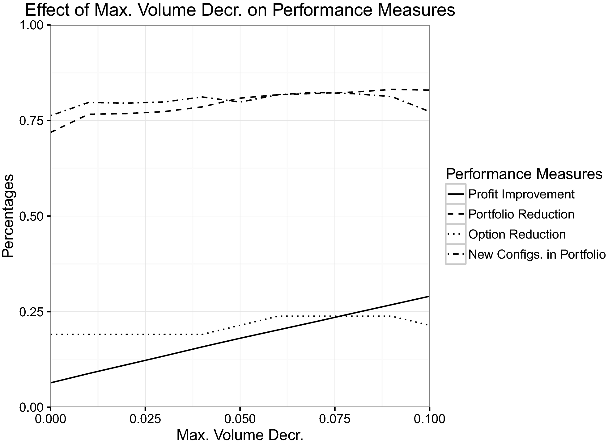
Maximum Sales Volume Decrease vs. Other Outputs

Insights Related to Cost of Complexity

Section 6.3.5 provided evidence for two insights that, although intuitive, had never been empirically verified by CAT. First, for some features, increasing the number of options decreases the costs of customer acquisition. Second, sales volume has a negative impact on product support costs (i.e., repair costs) and, at the same time, a positive impact on the cost of prime product inventory. In addition, we emphasize three complexity‐related takeaways from our analysis: (i) There are two types of impact of product portfolio complexity on cost, which need to be modeled separately: complexity driven by the number of options offered (VBC) and complexity driven by specific options (ABC); (ii) There are time lags and leads on the impact of complexity that may or may not be reflected in cost data is depending on the accounting methods used; (iii) Costs can be impacted in either direction (increase or decrease) by complexity.

Data Collection

As we collected data to implement and run our models, we found some data particularly useful, while there were other instances when we wished we had certain types of data that were not available, forcing us to go with the next‐best thing. Hence, as an added insight, we believe that tracking the following data, whenever possible and practical, would enhance a company's ability to improve their product portfolio: (i) Whether or not the product purchased by a customer was the one she originally had in mind to buy and, if not, record both the original choice and the final purchase; (ii) Record what options/features the product support costs are associated with. Having this data could have revealed that some options had an ABC effect on the cost pool.

Conclusion

We present a three‐step procedure to restructure a product line, demonstrating its successful application on the Backhoe Loader line at CAT. Our methodology hinges on (i) the construction of migration lists to capture customer preferences and willingness to substitute; (ii) explicitly capturing the (positive and negative) cost of complexity of a specific product line across different functional areas; and (iii) integrating these tools within a mathematical programming framework to produce a final product line. One of the greatest strengths of our methodology is its flexibility—each step can be tailored to a company's particular setting, data availability and strategic needs, so long as it produces the necessary output for the next step.

CAT's lane strategy has continued to evolve, for example, Thomson Reuters (2014) discusses a new variation in which lanes may contain only partially completed machines, which can be finished to customer order as needed. Ideas such as these offer opportunities to extend our work to new problem domains—analytically characterizing the performance of such a delayed differentiation strategy is an exciting and challenging problem.

Outside of CAT, our work can be extended in several directions. First, explicit experimental validation of our empirical models—in particular our migration list approach—would be of value. While this approach has been successfully applied in the construction equipment industry, further study could help establish how it could be applied in other sectors, and what changes might be necessary. For example, we set the list lengths based on consultation with CAT executives. A better understanding of how long such lists really are, and how willing customers are to substitute (and whether there is any sort of explicit cost to this) would be of interest.

Second, as our methodology is applied to other settings, new constraints might need to be incorporated into our mathematical program. One of the benefits of our procedure is that our optimization model is flexible enough to accommodate such constraints. Nevertheless, how it performs in other settings needs to be established.

Finally, the central thrust of this study has considered the trade‐off between cost of complexity and product line breadth. CAT has found what they believe to be the correct trade‐off, which entailed a dramatic reduction in their product line. Different companies, in different industries, will have to answer this question for themselves. It is our hope that the methods we present in our study can likewise help them find the answers they seek.

Footnotes

Alternatively, one can refine this approach by keeping the time lags in the model and computing the net present value of future cash flows.

Note that randomness in our choice model is restricted to the generation of option utilities and reservation values, which influence the construction of customer migration lists. Once created, these (fixed) lists serve as input to a deterministic optimization algorithm. Thus, we refer to our model as being “randomized”, as opposed to a random choice model, which typically has a different meaning.

Some data is masked to preserve confidentiality. The signs and magnitudes have been preserved.

CAT did not explain the rationale behind Equation ; they just asked us to enforce this requirement.

We describe this process in great detail in Appendix S1 in section 2.

Please note that even without markups, we enforce the 9 types of lists, taking wtp into account. We do this assuming that the company would first solve this no‐markup version of the problem to find a solution with a higher complexity cost reduction; and once the optimal portfolio and lane assignments are decided, they can increase prices because they already know people are willing to pay a little premium.

Please refer to section 2 of Appendix S1 for the plots illustrating this and following observations.

References

1.

Alptekinoglu A. Corbett C. . 2008. Mass customization vs. mass production: Variety and price competition. Manuf. Serv. Oper. Manag. 10(2): 204–217.

Go to Reference

2.

Anderson S. 1995. Measuring the impact of product mix heterogeneity on manufacturing overhead cost. Accoun. Rev. 70(3): 363–387.

Go to Reference

3.

Banker R. Potter G. Schroederr R. . 1995. An empirical analysis of manufacturing overhead cost drivers. J. Accoun. Econ. 19: 115–137.

Go to Reference

4.

Belloni A. Freund R. Selove M. Simester D. . 2008. Optimizing product line designs: Efficient methods and comparisons. Management Sci. 54(9): 1544–1552.

Go to Reference

5.

Bitran G. Ferrer J.‐C. . 2007. On pricing and composition of bundles. Prod. Oper. Manag. 16(1): 93–108.

Go to Reference

6.

Broniarczyk S. Hoyer W. McAlister L. . 1998. Consumers’ perceptions of the assortment offered in a grocery category: The impact of item reduction. J. Market. Res. 35: 166–176.

Go to Reference

7.

Chen K. Hausman W. . 2000. Technical note: Mathematical properties of the optimal product line selection problem using choice‐based conjoint analysis. Management Sci. 46(2): 327–332.

Go to Reference

8.

Chen Y. Vakharia A. Alptekinoglu A. . 2008. Product portfolio strategies: The case of multifunction products. Prod. Oper. Manag. 17(6): 587–598.

Go to Reference

9.

Chen Y. Carillo J. Vakharia A. Sin P. . 2010. Fusion product planning: A market offering perspective. Decis. Sci. 41(2): 325–353.

Go to Reference

10.

Chong J. Ho T. Tang C. S. . 1998. Product structure, brand width, and brand share. Ho T. Tang C. S. , eds. Product Variety Management: Research Advances. Kluwer Academic Publishers, New York, 39–64.

Go to Reference

11.

Fisher M. Ittner C. 1999. The impact of product variety on automobile assembly operations: Empirical evidence and simulation analysis. Management Sci. 45(6): 771–786.

Go to Reference

12.

Fisher M. Vaidyanathan R. . 2011. An algorithm and demand estimation procedure for retail as‐ sortment optimization. Working paper, University of Pennsylvania.

+ Show References

13.

Foster G. Gupta M. . 1990. Manufacturing overhead cost driver analysis. J. Accoun. Econ. 12: 309–337.

Go to Reference

14.

Fruchter G. Fligler A. Winer R. . 2006. Optimal product line design: Genetic algorithm approach to mitigate cannibalization. J. Optimiz. Theory Appl. 131(2): 227–244.

Go to Reference

15.

Greene W. H. 2000. Econometric Analysis, 4th edn. Prentice Hall, New Jersey.

+ Show References

16.

Guadagni P. M. Little J. D. C. . 1983. A logit model of brand choice calibrated on scanner data. Market. Sci. 2(3): 203–238.

Go to Reference

17.

Hauser J. R. Rao V. . 2004. Conjoint analysis, related modeling, and applications. Wind J. Green P. , eds. Advances in Market Research and Modeling: Progress and Prospects. Kluwer Academic Publishers, Boston, MA, 141–168.

Go to Reference

18.

Kok G. Fisher M. . 2007. Demand estimation and assortment optimization under substitution: Methodology and applications. Oper. Res. 55(6): 1001–1021.

Go to Reference

19.

Kok G. Fisher M. Vaidyanathan R. . 2009. Assortment planning: Review of literature and industry practice. Agrawal N. Smith S. , eds. Retail Supply Chain Management. Kluwer Academic Publishers, Amsterdam, The Netherlands, 1–55.

Go to Reference

20.

Marriott K. Stuckey P. . 1998. Programming with Constraints: An Introduction. MIT Press, Cambridge, MA.

Go to Reference

21.

Rash E. Kempf K. . 2012. Product line design and scheduling at Intel. Interfaces 42(5), 425–436.

Go to Reference

22.

Saaty T. L . 1980. The Analytic Hierarchy Process. McGraw‐Hill Book Co., New York.

Go to Reference

23.

Schoen C. 2010. On the optimal product line selection problem with price discrimination. Management Sci. 56(5): 896–902.

Go to Reference

24.

Tang C. 2010. A review of marketing‐operations interface models: From co‐existence to coordination and collaboration. Int. J. Prod. Econ. 125(1): 22–40.

Go to Reference

25.

Tang C. Yin R. . 2010. The implications of costs, capacity, and competition on product line selection. Eur. J. Oper. Res. 200(2): 439–450.

Go to Reference

26.

Thomson Reuters. Caterpillar Inc. 2014. Analyst Meeting at ConExpo edited transcript, 2014.

+ Show References

27.

Wang X. Camm J. Curry D. . 2009. A branch‐and‐price approach to the share‐of‐choice product line design problem managing product variety. Management Sci. 55(10): 1718–1728.

Go to Reference

28.

Ward J. Zhang B. Jain S. Fry C. Olavson T. Mishal H. Amaral J. Beyer D. Brecht A. Cargille B. Chadinha R. Chou K. DeNyse G. Feng Q. Padovani C. Raj S. Sunderbruch K. Tarjan R. Venkatraman K. Woods J. Zhou J. . 2010. HP transforms product portfolio management with operations research. Interfaces 40(1): 17–32.

Go to Reference

29.

Yunes T. H. Napolitano D. Scheller‐Wolf A. Tayur S. . 2007. Building efficient product portfolios at John Deere and Company. Oper. Res. 55(4): 615–629.

+ Show References