Integrated Commodity Inventory Management and Financial Hedging: A Dynamic Mean‐Variance Analysis

Abstract

We consider a firm purchasing a storable raw material commodity from a spot market with volatile commodity prices and the access to an associated financial derivatives market. The purchased commodity is processed into an end product with uncertain demand and lost sales. The firm aims to integrate the inventory replenishment and financial hedging decisions to maximize the mean‐variance of terminal wealth over a finite horizon. Recognizing time‐inconsistency of mean‐variance criteria, we employ the dynamic programming approach to obtain a time‐consistent policy. Assuming no arbitrage in financial market, we show that the mean‐variance utility functions under the time‐consistent policy have a recursive representation which enables us to readily characterize the structure of the time‐consistent policy. We analyze two types of hedging instruments, vanilla hedges and exotic hedges, and show that inventory and financial hedging decisions can be separated in the presence of forward contracts and a myopic state‐dependent base stock policy is optimal. The optimal hedging policy can be obtained by minimizing the variance of the hedging portfolio, the value of excess inventory and the profit‐to‐go as a function of future price. In the presence of a continuum of option strikes, we show how to construct custom exotic derivatives using forwards and options of all strikes to replicate the profit‐to‐go function. We then show the optimality of the time‐consistent policy under exotic hedge for the initial mean‐variance objective. We further investigate the dynamic interplay of inventories and financial hedge and show that they can be substitutes in a dynamic environment. Finally, we compare the performances in different hedging environments to discuss how financial hedges add value and provide a numerical study.

Keywords

inventory management financial hedging mean‐variance analysis time‐inconsistency

Introduction

The past decade has witnessed unprecedented volatility in commodity prices, threatening the survival of individual companies. For example, the crude oil price experienced tremendous fluctuations in recent years, falling from a peak of $115 per barrel in June 2014 down to under $35 in February 2016 but then up to about $50 in December 2016. According to a PwC survey of leading manufacturers, a large majority of senior executives said commodity price is crucial to a company's financial performance and many organizations were more proactive in managing commodity risks by focusing on improving operational efficiency and derivative hedging strategies (PwC 2008). For instance, the beverage producer Anheuser‐Busch uses exchange‐traded wheat futures and over‐the‐counter (OTC) aluminum swaps to hedge the risk of higher raw material prices. But financial hedging itself is a double‐edged sword and it needs to be integrated with operational strategies. In 2001, Ford announced $1 billion loss on precious metals inventory and forward‐contract agreements while Hewlett–Packard (HP) was able to cut commodity price risk using procurement risk management strategy based on a contract portfolio approach (Nagali et al. 2008).

Why should firms hedge? Merton H. Miller once said to an oil producer who resisted to use futures market, “When you hold inventory, non‐hedging is gambling. You gambled that the price of oil would not drop and you lost” (Miller 1997). A substantial literature in finance has provided the economic interpretations on why value‐maximizing firms may benefit from reducing profit variability and therefore engage in financial hedges as if they were risk averse. In their seminal paper, Smith and Stulz (1985) show that hedging, as part of firms’ financial policies, can reduce expected tax liability, bankruptcy costs, or compensation paid to risk‐averse managers, and they define hedging as the acquisition of financial assets that reduce the variance of the firm's payoffs. To capture those market imperfections and managerial risk aversion in a tractable fashion, instead of explicitly considering those factors (e.g., tax liability or bankruptcy), concave utility functions are often used to define firms’ decision criteria; see Chod et al. (2010) for a concave exponential function, and Gaur and Seshadri (2005) and Ding et al. (2007) for mean‐variance criteria. As argued by Smith and Stulz (1985) that the primary goal of hedging is to smooth cash flows, minimizing variability of cash flows is a natural objective for firms to develop hedging strategies. Duffie and Richardson (1991) also argue that hedging may reduce the expected costs arising from those market imperfections, and a simple hedging criterion, such as the minimum‐variance criterion, can be quite satisfactory from a practical point of view. Following these arguments, we adopt the mean‐variance criterion to analyze the joint replenishment and financial hedging problem.

The mean‐variance analysis of Markowitz (1952), that measures the risk of a portfolio with its variance, is seen as the cornerstone of modern portfolio theory and has been widely used in both academia and industry due to its simplicity and intuitive appeal (see, e.g., Basak and Chabakauri 2010, 2012, Hull 2008, Markowitz 1959, 1991 and the references therein). Eydeland and Wolyniec (2002) argue that the mean‐variance rule can serve as a proxy for other types of risk minimization rules. In particular, Levy and Levy (2004) show that the efficient sets of mean‐variance and prospect theory almost coincide and therefore one could use the mean‐variance rule to construct efficient portfolios under prospect theory, which justifies the robustness of the mean‐variance rule.

In this study, we address a joint inventory replenishment and financial hedging problem for a firm aiming to maximize mean‐variance of terminal wealth over a finite horizon. We attempt to answer the following questions: (i) What is the structure of the time‐consistent policy? (ii) When are the time‐consistent policies optimal for the initial mean‐variance objective? (iii) How do inventories and financial hedges interplay? and (iv) How do financial hedges add value for the firm?

More specifically, we consider a firm purchasing a storable commodity from a competitive physical spot market with the access to associated financial derivatives. The purchased commodity serves as a raw material which can be processed into an end product with fixed selling prices. The demand of the end product is random and unmet demand is treated as lost sales. The spot price evolves as a Markov process. The physical spot market and the associated financial derivatives market are both assumed to be liquid in that no transaction cost is incurred in trading. Moreover, we assume that there is no arbitrage opportunity in either the physical spot market or the financial market.

Note that the mean‐variance criterion is time‐inconsistent as the variance of terminal wealth evaluated at any point in time is greater than that of a later date, which provide incentives for the firm to deviate from the optimal policy for the initial objective. The time‐inconsistency problem has long been recognized in the economics literature (see, e.g., Caplin and Leahy 2006, Strotz 1956). However, since the time consistency is a basic requirement of rational decision making, Strotz (1956) argues that an investor should always choose the best plan among those that he will actually follow unless pre‐commitment is possible. Following Strotz (1956), Basak and Chabakauri (2010) use the dynamic programming approach to derive the time‐consistent policy for the dynamic mean‐variance portfolio problem. Using a similar approach, we develop a recursive formulation to derive a time‐consistent policy for the commodity inventory system.

We derive the time‐consistent policies in two types of hedging environments. When only exchanged‐traded vanilla derivative contracts, such as forwards and options, are used, we show that, with forward contracts maturing at next period, the joint replenishment and hedging optimization problem can be decomposed into two sub‐problems: a myopic inventory decision problem and a variance‐minimization portfolio optimization problem. We show that a myopic state‐dependent base‐stock policy is optimal. The optimal hedging decisions can be obtained by minimizing the variance associated with the expected future cash flows. We then show how to construct exotic derivative contracts with European calls and puts of all strikes to fully replicate the expected future cash flows, conditional on the next period's spot price. Note that exotic derivatives refer to all those non‐standard and tailor‐made derivative contracts that are mostly traded in OTC markets (Briys et al. 1998). We show that the optimal exotic hedge leads to the optimality of the time‐consistent policy for the initial objective function. We also investigate the interplay between inventories and financial hedges and show that financial hedges increase the inventory level in the last period, which is in line with the finding of the newsvendor literature (see, e.g., Gaur and Seshadri 2005), but may reduce the inventory level in the preceding periods, which implies that inventories and financial hedges may be substitutes. We further compare the performances of different hedging strategies and provide a numerical study to examine these results.

The rest of the study is organized as follows. Section 2 reviews the related literature. Section 3 describes the problem, discuss the time‐inconsistency issue and derive a recursive representation. Section 4 analyzes the structure of the time‐consistent policies under vanilla and exotic hedges. Section 5 studies the dynamic interplay between inventories and financial hedges. Section 6 presents a numerical study. Section 7 concludes the study. All the proofs are in the Appendix.

Related Literature

There exists a substantial literature on financial hedging in finance; see Sanda et al. (2013) for a review on the practice and recent developments of financial hedging in non‐financial firms. As the primary goal of hedging is to reduce cash‐flow variability (Smith and Stulz 1985), the minimum‐variance criterion is commonly used in practice (Duffie and Richardson 1991, Hull 2008). To capture the tradeoff between risk and return, Markowitz (1952) introduces mean‐variance criterion to portfolio risk management. In a complete market setting, Li and Ng (2000) provide a closed‐form solution for the optimal pre‐commitment policy that maximizes the mean‐variance objective at the initial date. However, due to the time‐inconsistency of the mean‐variance criteria, an investor may subsequently find it optimal to deviate from the initial policy if market conditions change in the future unless she is able to pre‐commit (Strotz 1956). Following Strotz (1956), Basak and Chabakauri (2010) employ a dynamic programming approach to derive a time‐consistent policy for a dynamic portfolio optimization problem in an incomplete market. Similarly, Basak and Chabakauri (2012) derive a time‐consistent variance‐minimization hedging strategy for a non‐tradable asset. We adopt a similar approach to derive a time‐consistent policy for a stochastic commodity inventory system where uncertain demand is a non‐tradable risk factor.

There is a growing body of literature on joint operational and financial risk management. See Kleindorfer (2009) and Turcic et al. (2015) for reviews of recent developments. Earlier studies focus on extending conventional models under risk‐neutral criteria to settings under risk‐averse criteria (see, e.g., Agrawal and Seshadri 2000, Bouakiz and Sobel 1992, Eeckhoudt et al. 1995). Recent developments on the joint operational and financial hedging problem focus on single‐period (newsvendor) settings. For example, Gaur and Seshadri (2005) consider a joint purchasing and financial hedging problem for a risk averse retailer with demand being correlated to a market index. They show that financial hedging increases the optimal inventory level, which implies that inventories and financial hedges are complements. Ding et al. (2007) consider a global manufacturer coordinating production and financial hedging strategies in the presence of exchange rate risk. Chod et al. (2010) examine the relationship between the operational flexibility and financial hedging in capacity investment decisions. They show that product flexibility and financial hedging tend to be complements (substitutes) when product demands are positively (negatively) correlated, whereas postponement flexibility is a substitute to financial hedging. Martínez‐de‐Albéniz and Simchi‐Levi (2006) study the mean‐variance tradeoffs for a manufacturer with a portfolio of option contracts.

There are only a few papers in multi‐period settings. With an additive exponential utility function that is time‐consistent, Chen et al. (2007) study an inventory system that integrates pricing, inventory control, consumption and financial hedging decisions. They characterize the optimal policy structure and show that the inventory and pricing decisions can be separated from the financial decisions, extending the separation theorem of Smith and Nau (1995) to an operational context. Note that their analysis implies that using financial hedges does not alter the optimal policy structure for inventory and pricing decisions when compared to the system without financial hedges. Using a similar framework, Geman and Ohana (2008) discuss time‐inconsistency of various risk measures and propose a time‐consistent criterion for a commodity portfolio problem.

More recently, Kouvelis et al. (2013) study a joint replenishment and financial hedging problem for a lost sales commodity inventory system under the criterion of maximizing mean‐variance of the net present value (NPV) of total cash flows over a finite horizon. Also recognizing the time‐inconsistency of such a criterion, they propose a stochastic program framework to derive a time‐consistent policy by solving a sequence of optimization problems. They analyze and compare single‐contract and multi‐contract hedging strategies and show that myopic base stock policies are optimal under forward hedge. Note that the mean‐variance utilities evaluated in consecutive periods do not have a recursive form, which limits its tractability. While considering a similar commodity inventory system, different from Kouvelis et al. (2013), we adopt the criterion of maximizing mean‐variance of terminal wealth. Note that although decision criteria based on NPV are prevalent in operations literature, the criteria based on terminal wealth are more common in portfolio theory (see, e.g., Back 2017, Basak and Chabakauri 2010, Duffie and Richardson 1991 and references therein). Following Basak and Chabakauri (2010), we develop a recursive representation for the mean‐variance utilities evaluated in consecutive periods, which allows us to derive a time‐consistent policy by backward induction. Compared to Kouvelis et al. (2013), our approach has better analytical tractability and computational efficiency. In particular, under exotic hedge, we show that the time‐consistent policy is indeed optimal for the initial objective. To our best knowledge, it is the first attempt to show that a time‐inconsistent criterion can have a time‐consistent optimal policy in the presence of non‐tradable risk. Moreover, we analyze the interplay between inventories and financial hedges and identify a condition under which inventories and financial hedges may be substitutes while Kouvelis et al. (2013) only discuss it in a numerical study.

In summary, our contributions to this literature are twofold. First, we explicitly address time‐inconsistency in the joint inventory and financial hedging problem in the mean‐variance framework. We employ the dynamic programming approach to derive the time‐consistent policies and show that when the financial market is reasonably complete, such as with a continuum of option strikes, the time‐consistent policy is also optimal in the admissible policy set. Second, our analysis sheds new light into effective commodity risk management practices: Inventory is used to hedge demand (quantity) risk while financial derivatives are used to hedge the price risk. The inventory replenishment decisions can be separated from financial hedging decisions and a state‐dependent myopic base stock policy is optimal. The optimal hedging policy consists of a forward hedge to offset the price risk related to the expected leftover inventory of the current period and a portfolio of financial derivatives to hedge the cash flows related to future decisions. Financial hedging does affect inventory policies and often simplifies them. However, optimal financial hedging strategies are heavily dependent on inventory policies as they determine future cash flows. In other words, inventory decisions can be separated from financial hedging decisions, but not the other way around.

The Model

Problem Description

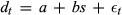
Consider a firm purchasing a storable commodity from a volatile spot market as a price taker. This commodity serves as a raw material which can be processed into an end product with uncertain demand and fixed selling prices. The processing is on demand basis, which implies that only the raw material inventory is held. Assume that there exists a spot market and an associated financial market for financial derivative contracts written on the spot price. The inventory is reviewed periodically and the periods are indexed by t = 0, 1, 2, …, T + 1. Period 0 is the beginning period and period T + 1 is the ending period. The firm serves the demand occurring in period t = 1, …, T, denoted by

d_{t}

, with a fixed unit selling price r _t. Note that when there exists a processing cost, r _t can also be seen as the unit net profit, which is equal to the unit selling price net of unit processing cost. Unmet demand is lost. The excess inventory is carried over to the next period and incurs a holding cost h _t for each unit of inventory.

Demand in each period may depend on the spot price. Without loss of generality, we assume that the support of demand is

R_{+}

. Let Φ_t(·¦s) and ϕ _t(·¦s) be the distribution and density functions of demand given a spot price s. Assume that Φ_t(ξ, s) is twice differentiable in (ξ, s). For example, a special case of the demand model has the additive linear form of

d_{t} = a + b s + ϵ_{t}

, where ε _t is an error term with a distribution independent of s such that E[ε _t] = 0 and

E [ϵ^{2}] < \infty

(see, e.g., Gaur and Seshadri 2005). An alternative model that is commonly used has the multiplicative form

d_{t} = e^{a + b s} ϵ_{t}

where ε _t is non‐negative random variable with a distribution independent of s.

We assume that this commodity can be sold to or bought from the spot market at spot price at the beginning of each period. The replenishment lead time is zero. Assume that the commodity spot market is liquid in the sense that there is no transaction cost and the bid–ask spread is zero. Let S _t be the spot price at the beginning of period t. Denote by s the realization of the spot price. The spot price process {S _t, t = 0, 1, …, T} is a Markov process. Let E[·] be the expectation operator under the subjective probability measure and E _t[·] = E[·¦S _t = s] be the conditional expectation operator. According to the competitive storage theory, the commodity price satisfies the following no‐arbitrage condition (see, e.g., Routledge et al. 2000, Williams and Wright 1991, Working 1948).

s + h_{t} - α E [S_{t + 1} | S_{t} = s] \geq 0,

where α is the risk‐free discount factor. Following Chen et al. (2007), we assume that the firm has access to a capital market for borrowing and lending any amount of cash with a risk‐free saving and borrowing interest rate r _f such that

α = \frac{1}{1 + r_{f}}

We assume that the derivatives market is frictionless in that the firm can buy or sell as many shares of a derivative contract as desired at the market price without incurring any transactional cost. In addition, all the relevant financial derivatives (e.g., forwards/futures and options) are written on the spot price of the underlying commodity. Let

A_{t}

denote a hedging portfolio that specifies a portfolio of derivatives held from period t to period t + 1, and

A_{t}

the set of feasible hedging portfolios in period t. The specification of

A_{t}

depends on the types of underlying financial derivatives that are available in the market. For example, if only forward contracts maturing at next period are available in the market, then a feasible hedging portfolio consists of certain number of such forward contracts to be bought (when the quantity is positive) or sold (when the quantity is negative). Define

H_{t}^{A_{t}} (S_{t + 1} | S_{t})

as the return (or marked‐to‐market payoff) of the next period's spot price S _t+1 under a hedging portfolio

A_{t}

given the spot price S _t in period t, and let

H_{t}

be the set of profit functions under feasible hedging portfolios in

A_{t}

. For convenience, we drop the superscript

A_{t}

and the argument S _t and simply use H _t(S _t+1) to represent a hedging portfolio. Hence the hedging decision in period t amounts to choosing a profit function H _t from

H_{t}

Following Froot et al. (1993), Gaur and Seshadri (2005) and Chod et al. (2010), we assume that the expected payoff of the financial hedging portfolio is zero, i.e., E _t[H _t(S _t+1)] = 0. Any violation of such an assumption implies that there exist speculative opportunities from financial hedging. From an operational manager's perspective, the main goal of trading financial assets is to hedge the risk in the operating profit due to the commodity price volatility, not to gain profit through speculation in the financial markets. Most firms do not allow managers to engage in such speculative behavior. As the goal of this research is to provide insights into how firms should manage the variations of operating profits using financial hedging, we use this assumption to eliminate the speculative motive in our analysis. Such a treatment is also commonly seen in finance literature (see, e.g., Brown and Toft 2002, Geman and Ohana 2008). Nevertheless, we will relax this assumption to allow non‐zero expected profits (i.e., arbitrage trading opportunities) from financial hedging in section 8.4 where we show that our structural results remain true, and thus our results are robust to this assumption.

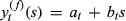
Our assumptions on the joint probability space of the demand and spot price are in line with the assumption of “partial complete market” by Smith and Nau (1995). See Chen et al. (2007) and Kouvelis et al. (2013) for more discussion on it. The forward prices are determined by the expected spot price at maturity of the contract. Let f _t,τ(s) be the forward price quoted in period t and for delivery in period τ ≥ t given the spot price at t, s. In particular, f _t,τ(s) = E _t[S _τ] and f _t,t = S _t.

Mean‐Variance Formulation and Time Inconsistency

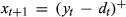
Note that in period 0 only hedging decision is made. From period 1 to T, a joint inventory and hedging decision is made. Let x _t be the inventory level at the beginning of period t and y _t be the order‐up‐to level in period t such that

y_{t} \in R_{+}

. The sequence of events in each period t > 0 is as following: (i) observe the spot price S _t = s and obtain the payoff of last period's financial hedge H _t−1(S _t); (ii) place an order y _t − x _t (bid if y _t > x _t or ask if y _t < x _t) from spot market, and choose a hedging portfolio H _t which matures at the next period; (iii) demand

d_{t}

occurs; and (iv) holding costs are incurred for ending inventory of the level

{(y_{t} - d_{t})}^{+}

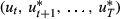
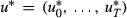
Denote by u _t = (y _t, H _t) be a feasible joint strategy in period t and u = (u ₀, …, u _T) an admissible policy. Let

U

be the set of admissible joint replenishment and financial hedging policies with y _t ≥ 0 for t = 1, …, T and

H_{t} \in H_{t}

for t = 0, …, T. For any

u \in U

, the dynamics of inventory level are

x_{t + 1} = {(y_{t} - d_{t})}^{+}, t = 1, \dots, T .

For simplicity, assume that the initial inventory levels in periods 0 and 1 are zero (i.e., x ₁ = x ₀ = 0) and y ₀ = 0. Then the operating profit in period 0 is zero (i.e.,

{\tilde{π}}_{0} = 0

) and we have

\begin{matrix} {\tilde{π}}_{t} (x_{t}, y_{t}, S_{t}) = & r_{t} min (y_{t}, d_{t}) - S_{t} (y_{t} - x_{t}) \\ - h_{t} {(y_{t} - d_{t})}^{+}, t = 1, 2, \dots, T . \end{matrix}

Since there is no any decision in period T + 1, the operating profit function of period T + 1 is a function of inventory level and spot price, defined as

{\tilde{π}}_{T + 1} (x_{T + 1}, S_{T + 1}) = x_{T + 1} S_{T + 1}

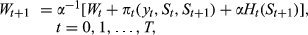
Let W ₀ be the initial wealth level of the planning horizon such that W ₀ ≥ 0. Let

{\tilde{W}}_{t}

be the initial wealth at the beginning of period t, t = 1, …, T + 1. Under a joint inventory and hedging strategy, the dynamics of wealth are represented by

{\tilde{W}}_{t + 1} = α^{- 1} [{\tilde{W}}_{t} + {\tilde{π}}_{t} (x_{t}, y_{t}, S_{t})] + H_{t} (S_{t + 1}), t = 1, \dots, T

and the terminal wealth is expressed as

\begin{matrix} {\tilde{W}}_{T + 1} & = α^{- 1} [{\tilde{W}}_{T} + {\tilde{π}}_{T} (x_{T}, y_{T}, S_{T})] + S_{T + 1} x_{T + 1} \\ + H_{T} (S_{T + 1}) \\ = α^{- (T + 1)} W_{0} + \sum_{t = 1}^{T} α^{- (T + 1 - t)} [{\tilde{π}}_{t} (x_{t}, y_{t}, S_{t}) \\ + H_{t - 1} (S_{t})] + S_{T + 1} x_{T + 1} + H_{T} (S_{T + 1}) . \end{matrix}

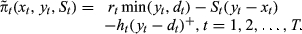
Note that the term S _t+1 x _t+1, which is equal to the market value of x _t+1 units of inventory, in the operating profit function of period t + 1,

{\tilde{π}}_{t + 1} (x_{t + 1}, y_{t + 1}, S_{t + 1})

, is associated with the inventory decision y _t in period t as

x_{t + 1} = {(y_{t} - d_{t})}^{+}

. For convenience, rearrange the revenue and cost terms directly associated with the inventory decision in each period into the following the profit functions

\begin{matrix} π_{t} (y_{t}, S_{t}, S_{t + 1}) & = r_{t} min (y_{t}, d_{t}) - S_{t} y_{t} - h_{t} {(y_{t} - d_{t})}^{+} \\ + α S_{t + 1} {(y_{t} - d_{t})}^{+}, \\ = (r_{t} - S_{t}) y_{t} - (r_{t} + h_{t} - α S_{t + 1}) {(y_{t} - d_{t})}^{+}, \\ t = 1, \dots, T, \end{matrix}

and π ₀(y ₀, S ₀, S ₁) = 0. Let π _t be the shorthand for the period‐t profit function. Different from the operating profit function

{\tilde{π}}_{t}

, π _t counts the net gain from the inventory decision y _t in period t using the sales revenue less the holding cost and plus the next‐period market value of the carryover inventory. Since the spot market is frictionless, the system works as if all the carryover inventory from last period were sold to the spot market at the beginning of each period. The optimal order‐up‐to level for each period does not depend on how much inventory is leftover from last period, which effectively allows us to separate the cash flows associated with the inventory decisions of consecutive periods. This is different from traditional inventory systems where the order‐up‐to level is bounded from below by the carryover inventory level.

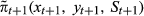
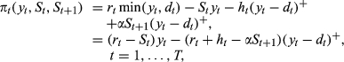
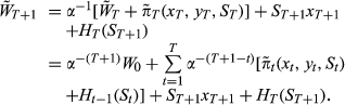
The dynamics of wealth process can be redefined as

\begin{matrix} W_{t + 1} & = α^{- 1} [W_{t} + π_{t} (y_{t}, S_{t}, S_{t + 1}) + α H_{t} (S_{t + 1})], \\ t = 0, 1, \dots, T, \end{matrix}

with the terminal wealth

\begin{matrix} W_{T + 1} & = {\tilde{W}}_{T + 1} = α^{- (T + 1)} W_{0} \\ + \sum_{t = 0}^{T} α^{- (T + 1 - t)} [π_{t} + α H_{t} (S_{t + 1})] . \end{matrix}

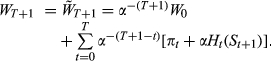
In the initial period 0, the firm's goal is to maximize the mean‐variance of terminal wealth accumulated over the whole planning horizon:

max_{u \in U} {U_{0} \equiv E_{0} [W_{T + 1}] - λ {Var}_{0} [W_{T + 1}]}

where the coefficient λ ≥ 0 represents the degree of the risk aversion. The optimal policy for the initial problem 4, denoted by u ⁽⁰⁾, is also called pre‐committed policy (Strotz 1956) or global optimal policy (Cui et al. 2017). However, such a policy may not be able to be implemented by a rational firm due to the time‐inconsistency of mean‐variance criteria and the firm has incentive to deviate from this initially optimal policy in later periods (Basak and Chabakauri 2010, Caplin and Leahy 2006, Strotz 1956). The root cause of the time‐inconsistency of mean‐variance criteria is the failure of the iterated‐expectation property of the variance measure. Intuitively speaking, sitting in each period, the firm perceives a greater variability of the terminal wealth than the anticipated variability in a future period. By the law‐of‐total‐variance (Weiss 2005), we have

\begin{matrix} {Var}_{t} (W_{T + 1}) & = E_{t} [{Var}_{t + 1} (W_{T + 1})] + {Var}_{t} [E_{t + 1} [W_{T + 1}]] \\ \geq E_{t} [{Var}_{t + 1} (W_{T + 1})], t = 0, 1, \dots, T . \end{matrix}

Here, the time‐t variance is larger than the expected value of time‐(t + 1) variance. Thus, the hedging strategy in time t should account not only for the expected time‐(t + 1) variance of the terminal wealth, but also the variance of time‐(t + 1) conditional expectation of the terminal wealth.

As time proceeds, upon receiving new market information and reviewing on‐hand inventory and wealth levels, the firm updates its mean‐variance objective

U_{t} \equiv E_{t} [W_{T + 1}] - λ {Var}_{t} [W_{T + 1}], t = 1, \dots, T .

Then these mean‐variance objectives evaluated in consecutive periods satisfy the following recursion

U_{t} = E_{t} [U_{t + 1}] - λ {Var}_{t} [E_{t + 1} [W_{T + 1}]], t = 0, \dots, T .

That is, the expected mean‐variance objective evaluated in time t can be expressed as its expected future value plus a variance adjustment term. This explains why the mean‐variance criterion of Equation 4 is time‐inconsistent: for any period, the policy that consists of joint replenishment and hedging decisions from period t + 1 onward to maximize future mean‐variance utility U _t+1 may not maximize the period‐t mean‐variance utility function U _t as the adjustment term may depend on future decisions, which drives the firm to deviate from its initially optimal policy.

Time consistency is a basic requirement of rational decision makers. Strotz (1956) argues that, when recognizing time‐inconsistency of mean‐variance criteria, the firm making decisions at any point in time should take account of the strategies it will actually execute in the future, even though those future decisions may not be optimal for its initial objective of Equation 4. Hence, it is rational for the firm to adopt a time‐consistent policy under which the firm optimally chooses the decisions at any point in time to maximize the mean‐variance of terminal wealth evaluated in that time, taking into account that he or she will act optimally in the future with respect to the mean‐variance of terminal wealth to be reevaluated in the future. We then follow Strotz (1956) and Basak and Chabakauri (2010) to employ the dynamic programming approach to derive a time‐consistent policy.

Dynamic Programming Formulation for Time‐Consistent Policies

We now present the approach to derive the time‐consistent policy. In this approach, the firm's dynamic optimization problem can be viewed as an intrapersonal sequential game such that the firm in each period acts as a Stackelberg leader and chooses the best strategy in this period while taking into account its best responses in future periods, and the corresponding sub‐game perfect Nash equilibrium policy is a time‐consistent policy (Basak and Chabakauri 2010, Cui et al. 2017).

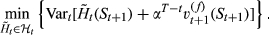
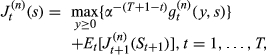
More specifically, for each period t, the firm solves the following optimization problems:

max_{u_{t} \in R_{+} \times H_{t}} \{E_{t} [W_{T + 1}^{(u_{t}, u_{t + 1}^{*}, \dots, u_{T}^{*})}] - λ {Var}_{t} [W_{T + 1}^{(u_{t}, u_{t + 1}^{*}, \dots, u_{T}^{*})}]\},

where u _t = (y _t, H _t) is a feasible solution in period t,

u_{t + 1}^{*}, \dots, u_{T}^{*}

are the optimal decision rules (as functions of state variables) that are obtained by solving the optimization problems 7 from period t + 1 onward by backward induction, and

W_{T + 1}^{(u_{t}, u_{t + 1}^{*}, \dots, u_{T}^{*})}

denotes the terminal wealth under the policy

(u_{t}, u_{t + 1}^{*}, \dots, u_{T}^{*})

. Denote by

u^{*} = (u_{0}^{*}, \dots, u_{T}^{*})

the resulting time‐consistent policy. Note that due to the time‐inconsistency, u* may not be a global optimal policy for the initial problem 4.

Let

{\tilde{J}}_{t} (W_{t}, s)

be the mean‐variance utility (also called value function) under the time‐consistent policy u* given the wealth level and spot price at the beginning of period t, (W _t, s), such that

{\tilde{J}}_{t} (W_{t}, s) = E_{t} [W_{T + 1}^{(u_{t}^{*}, u_{t + 1}^{*}, \dots, u_{T}^{*})}] - λ {Var}_{t} [W_{T + 1}^{(u_{t}^{*}, u_{t + 1}^{*}, \dots, u_{T}^{*})}] .

Applying recursive representation of the objective function 6, we have the following recursion:

{\tilde{J}}_{t} (W_{t}, s) = max_{u_{t} \in R_{+} \times H_{t}} \{E_{t} [{\tilde{J}}_{t + 1} (W_{t + 1}, S_{t + 1})] - λ {Var}_{t} [E_{t + 1} [W_{T}^{(u_{t}, u_{t + 1}^{*}, \dots, u_{T}^{*})}]]\} .

The following proposition further develops the recursion 8 as a bi‐level recursive representation.

Proposition 1

${\tilde{J}}_{0} (W_{0}, s)$
satisfies the following recursive equation:
$\begin{matrix} {\tilde{J}}_{0} (W_{0}, s) & = E_{0} [{\tilde{J}}_{1} (W_{1}, S_{1})] - λ min_{H_{0} \in H_{0}} {Var}_{0} \\ [α^{- T} H_{0} (S_{1}) + v_{1} (S_{1})] . \end{matrix}$
For t = 1, …, T,
${\tilde{J}}_{t} (W_{t}, s)$
satisfies the following recursive equation:
$\begin{matrix} {\tilde{J}}_{t} (W_{t}, s) & = max_{y_{t} \geq 0, H_{t} \in H_{t}} {E_{t} [{\tilde{J}}_{t + 1} (W_{t + 1}, S_{t + 1})] \\ - λ {Var}_{t} [α^{- (T + 1 - t)} [π_{t} (y_{t}, s, S_{t + 1}) \\ + α H_{t} (S_{t + 1})] + v_{t + 1} (S_{t + 1})]}, \end{matrix}$
where
${\tilde{J}}_{T + 1} (W_{T + 1}, s) = W_{T + 1}$
and v _t(s) is the expected operating profit function (accounted from period t to period T + 1) and satisfies the following recursive equation:
$v_{t} (s) = E_{t} [α^{- (T + 1 - t)} π_{t} (y_{t}^{} (s), S_{t}, S_{t + 1})] + E_{t} [v_{t + 1} (S_{t + 1})],$
with the terminal value v _T+1(s) = 0 and the optimal state‐dependent order‐up‐to level
$y_{t}^{} (s)$
.

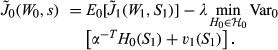
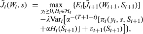
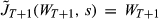
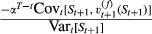
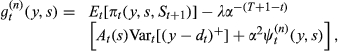
Proposition 1 shows a bi‐level recursive representation of the value functions under the time‐consistent policy u*, including the recursive representations for the mean‐variance utility functions and the expected operating profit functions. The following proposition further simplifies that the recursive representation 9 and 10 by separating the wealth level.

Proposition 2
The optimal mean‐variance utility function
${\tilde{J}}_{t} (W_{t}, s)$
can be decomposed as
${\tilde{J}}_{t} (W_{t}, s) = J_{t} (s) + α^{- (T + 1 - t)} W_{t}$
, where J _t satisfies the following optimality equations:
$J_{0} (s) = E_{0} [J_{1} (S_{1})] - λ α^{- 2 T} min_{H_{0} \in H_{0}} {Var}_{0} [α^{T} v_{1} (S_{1}) + H_{0} (S_{1})],$

$\begin{matrix} J_{t} (s) & = E_{t} [J_{t + 1} (S_{t + 1})] + max_{y \geq 0} {α^{- (T + 1 - t)} g_{t} (y, s)}, \\ t = 1, \dots, T, \end{matrix}$
where J _T+1(s) = 0 and
$\begin{matrix} g_{t} (y, s) & = E_{t} [π_{t} (y, s, S_{t + 1})] - λ α^{- (T + 1 - t)} \\ [A_{t} (s) Var [{(y - d_{t})}^{+}] + α^{2} ψ_{t} (y, s)], \end{matrix}$

$ψ_{t} (y, s) = min_{H_{t} \in H_{t}} \{{Var}_{t} [S_{t + 1} E_{t} [{(y - d_{t})}^{+}] + α^{T - t} v_{t + 1} (S_{t + 1}) + H_{t} (S_{t + 1})]\},$

with

$\begin{matrix} A_{t} (s) & = E_{t} [{(r_{t} + h_{t} - α S_{t})}^{2}] \\ = {(r_{t} + h_{t} - α f_{t} (s))}^{2} + α^{2} {Var}_{t} [S_{t + 1}] . \end{matrix}$

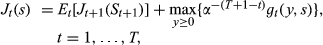
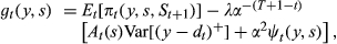
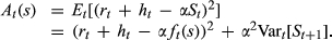
Note that Equations 12 and 13 are corresponding to Equations 9 and 10 with the separation of wealth level from the optimal mean‐variance utility functions. The separation of the wealth level allows us to separate J _t+1 from the optimization problem 10 and focus on the expected single period profit E _t[π _t(y, s, S _t+1)] and the time‐consistency variance adjustment term.

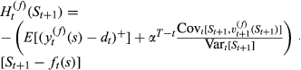
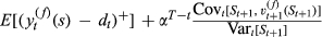
The optimality equation 13 implies that the inventory and financial hedging decisions depend only on the initial price and thus the current inventory decision will not affect next period's decisions. Moreover, the time‐consistent term is divided into two parts: the first one is related to the variance of leftover inventory (driven by demand uncertainty) that is carried over to the next period, and the second one is about the variance of the cash flows related to the spot price: the market value of expected carryover inventory, the period‐(t + 1) expected profit‐go‐to, and the payoff of financial hedging. This decomposition implies that the financial hedges are used to mitigate the price risk (by minimizing the variance of the cash flows related to the spot price of the next period), while the risk due to demand uncertainty (i.e., the variance of leftover inventory) cannot not be financially hedged. In other words, demand risk is hedged with physical inventory and price risk can be hedged by financial derivatives.

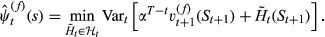
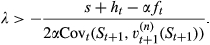
The optimal policy can be solved by backward induction from Equations 12 to 13. The optimality equation 13 also indicates that the joint inventory and financial hedging decision can be solved in two sequential steps. First, given any inventory decision y, the optimal hedging strategy is derived by solving the problem 15 from which we can see that the financial hedges should be constructed to offset the cash flow at the beginning of the next period,
$S_{t + 1} E_{t} [{(y - d_{t})}^{+}]$
, and the discounted profit‐to‐go α ^T−t v _t+1(S _t+1). Second, the optimal inventory decision is obtained by solving the problem in 13, given the optimal inventory level dependent hedging strategy.

Structure of Time‐Consistent Policies

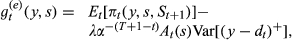
This section studies the structures of the time‐consistent joint replenishment and hedging policies under vanilla hedge and exotic hedges respectively. For convenience, we use superscripts (f) and (e) to indicate forward (and vanilla) hedges and exotic hedges, respectively, for relevant notation.

Hedging with Vanilla Derivatives

Vanilla derivatives include standard forward contracts and all those exchanged‐traded derivatives such as futures and options. The trading mechanisms of futures and forwards are similar though futures are traded on exchanges and forwards are traded in OTC markets. For simplicity, we ignore the difference between the futures and forwards. The following theorem characterizes the structure of the time‐consistent policy under vanilla hedge.

Theorem 1 Vanilla Hedges

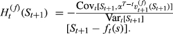
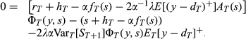
For periods t = 0, 1, …, T, suppose

H_{t}

contains at least the forwards maturing in the next period.

(a)
The time‐consistent replenishment policy is characterized by a myopic base‐stock policy and the optimal base‐stock levels derived from the following sub‐problems:
$\begin{matrix} max_{y \geq 0} {E_{t} [π_{t} (y_{t}, s, S_{t + 1})] - λ α^{- (T + 1 - t)} A_{t} (s) \\ {Var}_{t} [{(y - d_{t})}^{+}]}, t = 1, \dots, T . \end{matrix}$
In particular, if r _t≤s, the least optimal inventory level
$y_{t}^{(f)} (s) = 0$
; otherwise,
$y_{t}^{(f)} (s)$
is the unique solution of the following first‐order condition (FOC):
$\begin{matrix} [r_{t} + h_{t} - α f_{t} (s) - 2 α^{- (T + 1 - t)} λ E_{t} [{(y - d_{t})}^{+}] A_{t} (s)] \\ {\bar{Φ}}_{t} (y | s) - (s + h_{t} - α f_{t} (s)) = 0 . \end{matrix}$

(b)
The time‐consistent hedging policy is characterized by the hedging portfolios as follows. For each period t, the hedging portfolio consists of a position of shorting
$E [{(y_{t}^{(f)} (s) - d_{t})}^{+}]$
units of forwards maturing at next period and a portfolio
${\tilde{H}}_{t}^{(f)}$
derived from the following sub‐problem:
$min_{{\tilde{H}}_{t} \in H_{t}} \{{Var}_{t} [{\tilde{H}}_{t} (S_{t + 1}) + α^{T - t} v_{t + 1}^{(f)} (S_{t + 1})]\} .$

(c)
In particular, if only forwards maturing at next period are available, then
$\begin{matrix} {\tilde{H}}_{t}^{(f)} (S_{t + 1}) & = - α^{T - t} \frac{{Cov}_{t} [S_{t + 1}, v_{t + 1} (S_{t + 1})]}{{Var}_{t} [S_{t + 1}]} \\ [S_{t + 1} - f_{t} (s)], \end{matrix}$
and
$\begin{matrix} ψ_{t}^{(f)} (y, s) = \\ α^{2 (T - t)} [{Var}_{t} [v_{t + 1}^{(f)} (S_{t + 1})] - \frac{{({Cov}_{t} [S_{t + 1}, v_{t + 1}^{(f)} (S_{t + 1})])}^{2}}{{Var}_{t} [S_{t + 1}]}] . \end{matrix}$

Theorem 1 characterizes the time‐consistent policy in the presence of forward contracts. Specifically, part (a) shows that a myopic base‐stock policy is optimal and the optimal base stock level is either zero or the unique solution of Equation 17. Part (b) shows that the optimal hedging position of the forward contracts consists of two parts: Short
$E [{(y_{t}^{(f)} (s) - d_{t})}^{+}]$
units of forward and long
$- α^{T - t} \frac{{Cov}_{t} [S_{t + 1}, v_{t + 1}^{(f)} (S_{t + 1})]}{{Var}_{t} [S_{t + 1}]}$
(short if it is negative) units of forwards that mature next period. The first part of the portfolio offsets the variation due to the excess inventory carried over to next period and the second part is to hedge against the risk associated with the future cash flow,
$v_{t + 1}^{(f)} (S_{t + 1})$
. Note that the ratio
$\frac{- α^{T - t} {Cov}_{t} [S_{t + 1}, v_{t + 1}^{(f)} (S_{t + 1})]}{{Var}_{t} [S_{t + 1}]}$
is known as the optimal minimum variance hedge ratio in the literature for forward (futures) hedges (Hull 2008). The net forward hedging position is the combination of the two parts:
$\begin{matrix} H_{t}^{(f)} (S_{t + 1}) = \\ - (E [{(y_{t}^{(f)} (s) - d_{t})}^{+}] + α^{T - t} \frac{{Cov}_{t} [S_{t + 1}, v_{t + 1}^{(f)} (S_{t + 1})]}{{Var}_{t} [S_{t + 1}]}) \\ [S_{t + 1} - f_{t} (s)] \end{matrix} .$
It is a long (short) position if
$E [{(y_{t}^{(f)} (s) - d_{t})}^{+}] + α^{T - t} \frac{{Cov}_{t} [S_{t + 1}, v_{t + 1}^{(f)} (S_{t + 1})]}{{Var}_{t} [S_{t + 1}]}$
is negative (positive).

This theorem implies that, in the presence of the forward contract maturing at the next period, one could make the inventory decision independently, knowing that the risk associated with the expected excess inventory will be eliminated by a forward hedge. Then J _t can be rewritten as
$J_{t}^{(f)} (s) = α^{- (T + 1 - t)} {\hat{g}}_{t}^{(f)} (s) - λ α^{- 2 (T - t)} {\hat{ψ}}_{t}^{(f)} (s) + E_{t} [J_{t + 1}^{(f)} (S_{t + 1})],$

${\hat{g}}_{t}^{(f)} (s) = max_{y \geq 0} \{E_{t} [π_{t}] - λ α^{- (T + 1 - t)} A_{t} (s) {Var}_{t} [{(y - d_{t})}^{+}]\},$

${\hat{ψ}}_{t}^{(f)} (s) = min_{{\tilde{H}}_{t} \in H_{t}} {Var}_{t} [α^{T - t} v_{t + 1}^{(f)} (S_{t + 1}) + {\tilde{H}}_{t} (S_{t + 1})] .$
That is, the joint optimization problem (13)–(15) can be separated into two sub‐problems: One only concerns about optimal inventory decisions to handle the non‐tradable demand risk and the other only concerns about financial decisions to hedge against the tradable price risk. This separation allows us to compute the original dynamic program in four steps: (i) Derive the optimal myopic base‐stock level for each period by solving the inventory‐related sub‐problem 19; (ii) Compute the expected profit‐to‐go function v _t for all the periods; (iii) Compute the optimal portfolio
${\tilde{H}}_{t}^{(f)}$
of Equation 20 using the v _t; and (iv) Obtain the optimal hedging portfolio by combining the short position related to the expected excess inventory and
${\tilde{H}}_{t}^{(f)}$
. It is notable that with this separation and the assumption E _t[H _t(S _t+1)] = 0 the expected the expected profit‐to‐go function v _t is fully determined by the myopic basestock policy
$y_{t^{'}}^{(f)}, t^{'} = t, \dots, T$
, which in turn implies that
$v_{t}^{(f)}$
is unique and hence the optimal mean‐variance utility function
$J_{t}^{(f)}$
is unique.

This separation has an important practical implication. In practice, inventory decisions are made by operations managers while the hedging decisions are made by financial managers. Our result suggests that the management can allow the operations manager to manage inventory decisions separately from financial hedging decisions. But, when making the hedging decisions, the risk manager must take into account the optimal inventory policy to forecast the resulting future cash flow. Therefore, the financial hedges simplify the operations manager's task and help clarify the relationship between operations management and financial risk management within an organization.

Remark 1
The optimality of the myopic base stock policy is ensured by the forwards maturing in next period. Without the forward contract maturing at next period, the risk associated with carryover inventory cannot be perfectly hedged and therefore the determinant of the optimal base stock level
$y_{t}^{(f)} (s)$
depends on
$v_{t + 1}^{(f)}$
, which implies that the optimal base stock policy may not be myopic and the joint optimization problem may not be decomposed into two separate sub‐problems.

The following corollary follows immediately from Theorem 1.

Corollary 1
Suppose the demand is perfectly correlated to the spot price with the specification
$d_{t} = a_{t} + b_{t} s$
for constants a _t, b _t such that
$d_{t} \geq 0$
. Then, for t = 1, …, T, (a)

$y_{t}^{(f)} (s) = a_{t} + b_{t} s$
if r _t > s and
$y_{t}^{} (s) = 0$
if r _t ≤ s.
(b)

$v_{t}^{(f)} (s) = E_{t} [\sum_{τ = t}^{T} α^{τ - t} {(r_{τ} - S_{τ})}^{+} (a_{τ} + b_{τ} S_{τ})]$
.
(c)
If only forwards maturing at next period are available, then the optimal hedging portfolio is
$\begin{matrix} H_{t}^{(f)} (S_{t + 1}) & = - \frac{{Cov}_{t} [S_{t + 1}, α^{T - t} v_{t + 1}^{(f)} (S_{t + 1})]}{{Var}_{t} [S_{t + 1}]} \\ [S_{t + 1} - f_{t} (s)] . \end{matrix}$

(d)
If both call and put options contracts maturing at any future period are available and b _t = 0, i.e.,
$d_{t} = a_{t}$
, then the optimal hedging strategy in period t is to short a _τ units of put options with strike price r _τ and maturity date τ + 1 for τ = t + 1, …, T.

Corollary 1 shows that when the demand is perfectly correlated to the spot price, i.e., only price risk exists, the ordering quantity of each period is simply to order the demanded quantity. But v _t(s) is still nonlinear in s (due to the term (r _t − S _t)⁺), which implies that the price risk cannot be perfectly hedged by forward contracts. For deterministic demand, the price risk can be perfectly hedged by entering the short position in put options.

We next show the effect of the degree of risk aversion, represented by λ, on the inventory policy.

Corollary 2
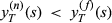
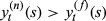
For all t, the optimal inventory decision
$y_{t}^{(f)} (s; λ)$
, is decreasing in λ.

Corollary 2 shows that the more risk‐averse firm orders less under forward hedge. In particular, when λ = 0 and r _t > s,
$y_{t}^{(f)} (s; λ)$
reduces to a newsvendor solution
$y_{t}^{NV} (s) = {\bar{Φ}}_{t}^{- 1} (\frac{s + h_{t} - α f_{t} (s)}{r_{t} + h_{t} - α f_{t} (s)}) .$

Hedging with Exotic Derivatives

In derivatives markets, since standard options contracts traded in exchanges normally have limited number of strikes, exotic derivatives* are normally structured by financial institutions in OTC markets to meet the precise needs of their clients to develop more sophisticated hedging strategies (Hull 2008). In finance literature, it is common to assume that there exists a continuum of options of all strikes as a proxy to a frictionless financial market (see, e.g., Carr and Madan 2001). Carr and Madan (2001) argue that, the assumption of a continuum of strikes is essentially the counterpart of the standard assumption of continuous trading, which serves as a reasonable approximation to a market environment where there is a large but finite number of European options strikes (e.g., options for S&P 500). In a single‐period hedging model, Carr and Madan (2001) show that a twice‐continuously differentiable payoff function can be replicated by a portfolio of a spectrum of European put and call options with a continuum of strikes, forwards, and risk‐less bonds.

We next follow Carr and Madan (2001) to construct an optimal exotic hedging strategy. To this end, we need to impose the following assumption on spot price.

Assumption 1
For all t and any real function v(·) which is twice differentiable almost everywhere, the conditional expectation E[v(S _t+1)¦S _t = s] is twice differentiable in s almost everywhere.

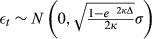
A common example of commodity price is the geometric Ornstein–Uhlenbeck process:
$d ln S = κ (α^{} - ln S) d t + σ d z^{} (t)$
where κ is the mean‐reverting rate, α ^* = η − σ ²/2 − γ is the risk adjusted long‐run mean (η is the long‐run mean and γ is the market price of risk) and z* is a Brownian motion under the risk neutral measure (Schwartz 1997). Assume the length of each period is equal to Δ. It follows from Schwartz (1997) that the discrete‐time dynamics of S _t+1 are of the form
$S_{t + 1} = exp (α^{} (1 - e^{- κ Δ}) + e^{- κ Δ} ln S_{t} + ϵ_{t + 1}),$
where
$ϵ_{t} \sim N (0, \sqrt{\frac{1 - e^{- 2 κ Δ}}{2 κ}} σ)$
. Apparently, for any twice differentiable function v with finite E[v ^′(S)] and E[v ^′′(S)], v(S _t+1) is twice differentiable in S _t and then the conditional expectation
$E [v (S_{t + 1}) | S_{t} = s] = E [v (s^{e^{- κ Δ}} exp (α^{} (1 - e^{- κ Δ}) + e^{- κ Δ} + ϵ_{t + 1}))]$
is twice differentiable in s.

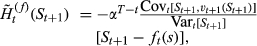
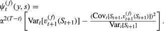
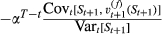
The following theorem characterizes the optimal policy structure under exotic hedge.

Theorem 2 Exotic Hedge

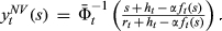
Suppose that there exist forwards and European calls and puts of all strikes, and Assumption 1 holds.

(a)
The time‐consistent replenishment policy under exotic hedge is identical to that under forward hedge as described in Theorem 1(a): For all t, if r _t ≤ s, the least optimal base‐stock level
$y_{t}^{(e)} (s) = 0$
; otherwise,
$y_{t}^{(e)} (s)$
is the unique solution of the following FOC:
$\begin{matrix} [r_{t} + h_{t} - α f_{t} (s) & - 2 α^{- (T + 1 - t)} λ E [{(y - d_{t})}^{+}] A_{t} (s)] \\ {\bar{Φ}}_{t} (y | s) - (s + h_{t} - α f_{t} (s)) = 0 . \end{matrix}$

(b)
The time‐consistent hedging policy under exotic hedge is characterized by the hedging portfolios as follows. For t = 0, …, T, the optimal hedging portfolio is to short
$E_{t} [{(y_{t}^{(e)} (s) - d_{t})}^{+}] + α^{T - t} {(v_{t + 1}^{(e)})}^{'} (s)$
units of forwards,
$α^{T - t} {(v_{t + 1}^{(e)})}^{″} (K) d K$
units of puts for all strikes K < s and
$α^{T - t} {(v_{t + 1}^{(e)})}^{″} (K) d K$
units of calls for all strikes K > s maturing at next period. That is,
$\begin{matrix} H_{t}^{(e)} (S_{t + 1}) = \\ - [(E_{t} [{(y_{t}^{(e)} (s) - d_{t})}^{+}] + α^{T - t} {(v_{t + 1}^{(e)})}^{'} (s)) [S_{t + 1} - f_{t} (s)] \\ + \int_{0}^{s} α^{T - t} {(v_{t + 1}^{(e)})}^{″} (K) [{(K - S_{t + 1})}^{+} - P_{t} (K)] d K \\ + \int_{s}^{\infty} α^{T - t} {(v_{t + 1}^{(e)})}^{″} (K) [{(S_{t + 1} - K)}^{+} - C_{t} (K)] d K], \end{matrix}$
where P _t(K)=E _t[(K−S _t+1)⁺] and C _t(K)=E _t[(S _t+1 −K)⁺].

Theorem 2 characterizes the structure of the time‐ shows that the optimal ordering policy under exotic hedge is the same as that under forward hedge: a myopic state‐dependent base‐stock policy is optimal.
$y_{t}^{(e)} (s)$
. Part (b) shows that the optimal hedging portfolio consists of two parts. The first part, similar to the forward hedge, is to take a short position in forwards maturing in next period to offset the price risk associated with the expected carryover inventory
$E_{t} [{(y_{t}^{(e)} (s) - d_{t})}^{+}]$
. The second part of the hedging strategy is related to the period‐(t + 1) profit‐to‐go function
$v_{t + 1}^{(e)} (S_{t + 1})$
that accounts for the expected cash flows from period t + 1 forward conditional on next period's spot price S _t+1. We follow Carr and Madan (2001) to decompose the profit‐to‐go function into three components which can be offset by a portfolio of the forwards and options. Specifically, the optimal hedging decision requires to short
$α^{T - t} {(v_{t + 1}^{(e)})}^{'} (s)$
units of forward (in addition to those related to inventory decision),
$α^{T - t} {(v_{t + 1}^{(e)})}^{″} (K) d K$
puts for all strikes K < s and
$α^{T - t} {(v_{t + 1}^{(e)})}^{″} (K) d K$
calls for all strikes K > s maturing at next period. As a result, under the optimal hedging strategy, the period‐(t + 1) profit‐to‐go function
$(v_{t + 1}^{(e)}) (S_{t + 1})$
is fully replicated by the constructed exotic hedging portfolio. That is, the variation driven by spot price S _t+1 can be fully eliminated under exotic hedge.

Then, under the optimal exotic hedging strategy, the Equation 14 is equal to
$\begin{matrix} g_{t}^{(e)} (y, s) = & E_{t} [π_{t} (y, s, S_{t + 1})] - \\ λ α^{- (T + 1 - t)} A_{t} (s) Var [{(y - d_{t})}^{+}], \end{matrix}$
where the second term only involves the variation driven by demand uncertainty, which further highlights the distinctive roles of inventories and financial hedges: the price risk is eliminated by exotic hedge while the demand risk is addressed by physical inventory.

We next show the optimality of the time‐consistent policy under exotic hedge for initial objective.

Theorem 3 Optimality of Time‐consistent Policies under Exotic Hedge

The time‐consistent policy under exotic hedge, characterized by Theorem 2, is optimal for the original mean‐variance optimization problem 4 in the initial period 0.

Note that although forward hedges are sufficient to separate the inventory decisions from financial hedges in the same period (Theorem 1) the future inventory decisions, which determine the profit‐to‐go function

v_{t + 1}^{(e)} (S_{t + 1})

in each period t, can still influence the current hedging decisions. The optimal inventory decisions from period t + 1 onward may not help minimize the variance when sitting in period t as the structure of

v_{t + 1}^{(e)} (S_{t + 1})

may restrict the minimum variance the forward hedges can achieve, which is also recognized by Basak and Chabakauri (2010). However, under exotic hedge, the expected profit‐to‐go

v_{t + 1}^{(e)} (S_{t + 1})

can be fully replicated by the hedging portfolio and the variance associated with the price risk is fully eliminated. Hence the replenishment decisions from period t + 1 onward are independent of the current decisions. We call such a separation the inter‐temporal separation. With the inter‐temporal separation, the time‐consistent policy is indeed optimal in the sense that future optimal decisions plus the current optimal decisions indeed minimize the mean‐variance of terminal wealth evaluated in the current period. Therefore, despite the time‐inconsistency of the objective function, the time‐consistent policies under exotic hedge can maximize the mean‐variance of terminal wealth evaluated in each period, including the objective function of 4. To the best of our knowledge, such a result is new to the literature.

Dynamic Interplay between Inventories and Financial Hedges

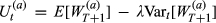
We now study the dynamic interplay between inventories and financial hedges. To this end, we consider the setting in the absence of financial hedges, which is described as a “no hedge” environment, indicated by the superscript (n). Then under the time‐consistent policy, we have

\begin{matrix} J_{t}^{(n)} (s) = & max_{y \geq 0} {α^{- (T + 1 - t)} g_{t}^{(n)} (y, s)} \\ + E_{t} [J_{t + 1}^{(n)} (S_{t + 1})], t = 1, \dots, T, \end{matrix}

where

\begin{matrix} g_{t}^{(n)} (y, s) = & E_{t} [π_{t} (y, s, S_{t + 1})] - λ α^{- (T + 1 - t)} \\ [A_{t} (s) {Var}_{t} [{(y - d_{t})}^{+}] + α^{2} ψ_{t}^{(n)} (y, s)], \end{matrix}

ψ_{t}^{(n)} (y, s) = {Var}_{t} [S_{t + 1} E_{t} [{(y - d_{t})}^{+}] + α^{T - t} v_{t + 1}^{(n)} (S_{t + 1})],

with

J_{T + 1}^{(n)} (s) = 0

. Let

y_{t}^{(n)} (s)

be the optimal inventory decision without the financial hedges.

Proposition 3

Suppose there is no financial hedge for period T. (a)

If r _T ≤ s, the optimal inventory decision

y_{T}^{(n)} (s) = 0

; otherwise, the optimal inventory decision

y_{T}^{(n)} (s)

satisfies the following first‐order condition:

\begin{matrix} 0 = & [r_{T} + h_{T} - α f_{T} (s) - 2 α^{- 1} λ E [{(y - d_{T})}^{+}] A_{T} (s)] \\ {\bar{Φ}}_{T} (y, s) - (s + h_{T} - α f_{T} (s)) \\ - 2 λ α {Var}_{T} [S_{T + 1}] Φ_{T} (y, s) E_{T} {[y - d_{T}]}^{+} . \end{matrix}

(b)

In particular, when r _T > s,

y_{T}^{(n)} (s) < y_{T}^{(f)} (s)

, i.e., the optimal order‐up‐to level under no hedge is lower than under forward hedge.

Part (a) characterizes the optimal inventory decision in period T. Part (b) shows that financial hedging, such as forward hedge, can result in a higher inventory level that no hedging does, which implies that inventories and financial hedges are complements in the last period. This insight is in line with that in newsvendor models (see, e.g., Ding et al. 2007, Gaur and Seshadri 2005).

However, for earlier periods before period T, inventories and financial hedges may no longer be complements. The following proposition identifies a condition that the inventory decisions under forward hedges are less than that under no hedge.

Proposition 4

For any period t = 1, …, T − 1, suppose there are no financial hedges and

y_{t}^{(f)} (s) > 0

. Then

y_{t}^{(n)} (s) > y_{t}^{(f)} (s)

if and only if

E [{(y_{t}^{(f)} (s) - d_{t})}^{+}] < - α^{T - t} \frac{{Cov}_{t} (S_{t + 1}, v_{t + 1}^{(n)} (S_{t + 1}))}{{Var}_{t} (S_{t + 1})} .

Proposition 4 shows that the optimal unhedged inventory decision can be greater than that under financial hedges in period t when inequality 28 holds. Note that

E [{(y_{t}^{(f)} (s) - d_{t})}^{+}]

is the expected carryover inventory under forward hedge and

- α^{T - t} \frac{{Cov}_{t} (S_{t + 1}, v_{t + 1}^{(n)} (S_{t + 1}))}{{Var}_{t} (S_{t + 1})}

is equal to the optimal hedging position for the future cash flows if forward contracts were used. Inequality 28 implies that the spot price S _t+1 is negatively correlated with the profit‐to‐go function

v_{t + 1}^{(n)} (S_{t + 1})

so that the carryover inventory can offset the variations of future cash flows. Proposition 4 implies that when the optimal forward position is greater that the expected carryover inventory level when the inventory decision is equal to

y_{t}^{(f)} (s)

, the firm has a motive to order more, as if purchasing more forwards, to further mitigate the variation of future cash flows.

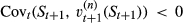
Intuitively, the expected profit of each period is a decreasing function of the purchasing price and thus the future cash flows may be negatively correlated to the spot price. To show that such a negative correlation does exist, we consider the following special case.

Proposition 5

For period t = 1, …, T, suppose the demand is perfectly negatively correlated with spot price with the form

d_{t} = {(a_{t} - b_{t} s)}^{+}, a_{t} > 0, b_{t} > 0

. Then

y_{t}^{(n)} > d_{t}

if and only if

λ > - \frac{s + h_{t} - α f_{t}}{2 α {Cov}_{t} (S_{t + 1}, v_{t + 1}^{(n)} (S_{t + 1}))} .

Note that

v_{t}^{(n)} (s) = E_{t} [\sum_{τ = t}^{T} α^{- (T + 1 - τ)} {(r_{τ} - S_{τ})}^{+} {(a - b S_{τ})}^{+}]

which is a strictly decreasing function of S _t = s. Clearly, S _t+1 and

v_{t + 1}^{(n)} (S_{t + 1})

are negatively correlated, i.e.,

{Cov}_{t} (S_{t + 1}, v_{t + 1}^{(n)} (S_{t + 1})) < 0

, which provides the motive to order more in period t to hedge the price risk for the cash flows from period t + 1 onward. Note that in the presence of financial hedges the optimal inventory policy is to order

d_{t}

units of inventory in each period t. Proposition 5 shows that, if the demand is perfectly negatively correlated with spot price and the risk‐aversion coefficient λ is sufficiently high, it is optimal to order more inventory than the demand in period t to hedge the future inventory risk.

The above two propositions shed new light into the relationship between physical inventories and financial hedges in dynamic inventory systems. If only the price risk associated with leftover inventory is of the concern in period T, financial hedges that eliminate the price allow the firm to focus on demand risk and therefore induce the firm to increase inventory level, which implies a complementary relationship. However, in the earlier periods, the firm is concern with not only the price risk associated with the leftover inventory but also that associated with future cash flows, the aggregate price risk may drive the firm to raise inventory level in the absence of financial hedges, which implies a substitute relationship.

We next analyze the effects of financial hedges on several financial performance indicators, namely, mean‐variance utility, mean and variance of terminal wealth.

Proposition 6

Let

U_{t}^{(a)} = E [W_{T + 1}^{(a)}] - λ {Var}_{t} [W_{T + 1}^{(a)}]

with a ∈ {n, f, e}.

(a)

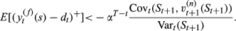
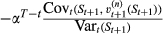
For each t = 1, …, T, the mean‐variance utilities under exotic hedge are greater than that under both forward hedge and no hedge, i.e.,

U_{t}^{(n)} \leq U_{t}^{(e)}

and

U_{t}^{(f)} \leq U_{t}^{(e)}

(b)

For each t = 1, …, T, the mean values of terminal wealth under forward hedge and exotic hedge are identical but the variances of terminal wealth under forward hedge are greater than that under exotic hedge, i.e.,

E_{t} [W_{T + 1}^{(f)}] = E_{t} [W_{T + 1}^{(e)}]

and

{Var}_{t} [W_{T + 1}^{(f)}] \geq {Var}_{t} [W_{T + 1}^{(e)}]

(c)

In particular, for period T,

U_{T}^{(n)} \leq U_{T}^{(f)} \leq U_{T}^{(e)}

E_{T} [W_{T + 1}^{(n)}] \leq E_{T} [W_{T + 1}^{(f)}] = E_{T} [W_{T + 1}^{(e)}]

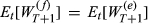
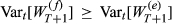
Proposition 6 shows that the exotic hedge results in higher mean‐variance utilities than the forward hedge and no hedge. The expected terminal wealth under exotic hedge and forward hedge are identical, which can be explained by the fact that the inventory policy under them are identical and the expected terminal wealth depends only on the inventory policy. In period T, exotic hedge and forward hedge lead to a higher inventory level and therefore a higher expected profit. In earlier periods, since the optimal inventory levels under no hedge may be higher (by Proposition 4), which leads to higher expected profits, it is unclear whether the expected values of terminal wealth evaluated in earlier periods under no hedge are greater or smaller than that under financial hedges. The variances of terminal wealth under exotic hedge are smaller than that under forward hedge, which is because the exotic hedge can fully eliminate the price risk associated with future cash flows while the forward hedge can only partially hedge it. But it is unclear whether the variances of terminal wealth under financial hedges are greater or smaller than that under no hedge.

In summary, in a dynamic commodity inventory system, financial hedging can add value by substituting physical inventories that are costly due to holding costs and more efficiently offsetting the variation driven by commodity spot prices. When the derivatives market is sufficiently complete in the sense that the firm can use exotic contracts to fully hedge the price risk, exotic hedging is more advantageous to no hedge and simple forward hedge.

A Numerical Study

The numerical study compares the best time‐consistent policies and their performances in different hedging environments: (i) forward hedge, (ii) exotic hedge, and (iii) no (financial) hedge.

Specifically, we consider a four‐period setting, i.e., T = 4, with the length of each period being Δ = 1. Assume that the risk‐adjusted spot price process follows the Geometric Mean‐Reverting process 22. We use the calibration of Schwartz (1997) for crude oil price to specify the parameters of the price process as κ = 0.428, η = 2.991, σ = 0.257, γ = 0.002. The demand is expressed as

d_{t} = μ_{d} + ϵ_{t}

where μ _d is the mean of the demand and the error terms ε _t are i.i.d. normally distributed with mean 0 and variance

σ_{d}^{2}

. Set μ _d = 10 and σ _d = 5. The initial wealth level is assumed to be zero. The other cost and model parameters are r _t = 50, h _t = 5, α = 0.9 and λ = 0.01. Employing the standard value iteration approach for dynamic programming, we compute the optimal policies using the corresponding optimality equations. The results are demonstrated in Figures 1–3.

Figure 1

Ordering Decisions [Color figure can be viewed at wileyonlinelibrary.com]

Figure 2

Hedging Decisions [Color figure can be viewed at wileyonlinelibrary.com]

Figure 3

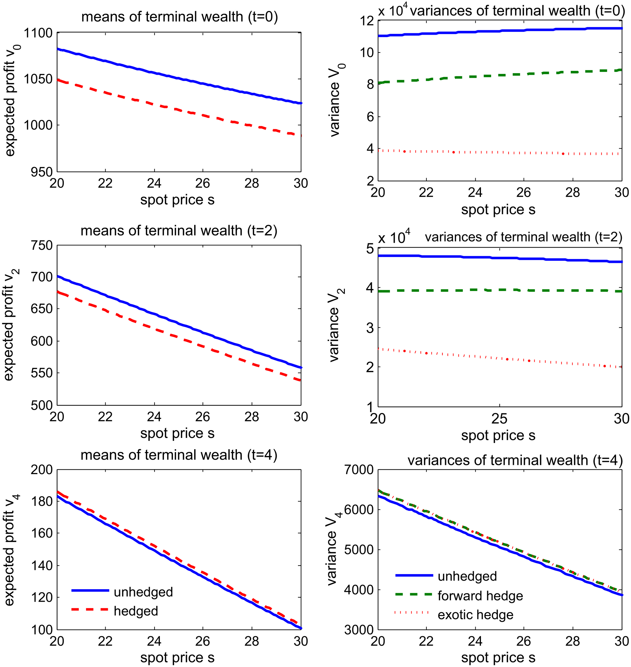
Mean‐Variance Performance of Terminal Wealth [Color figure can be viewed at wileyonlinelibrary.com]

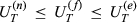
Figure 1 compares the optimal order‐up‐to levels with financial hedges or no hedge. Recall that the optimal inventory decisions under forward hedge and exotic hedge are identical. Comparing the hedged and unhedged inventory decisions, in the last decision period T = 4 the hedged order‐up‐to levels are greater than the unhedged ones whereas in the earlier periods the hedged ones are smaller. That is, financial hedges drive the firm to order more in the last period but order less in the earlier periods, which confirms our predictions in Propositions 3 and 5 and implies that inventories and financial hedges can be substitutes in dynamic environments.

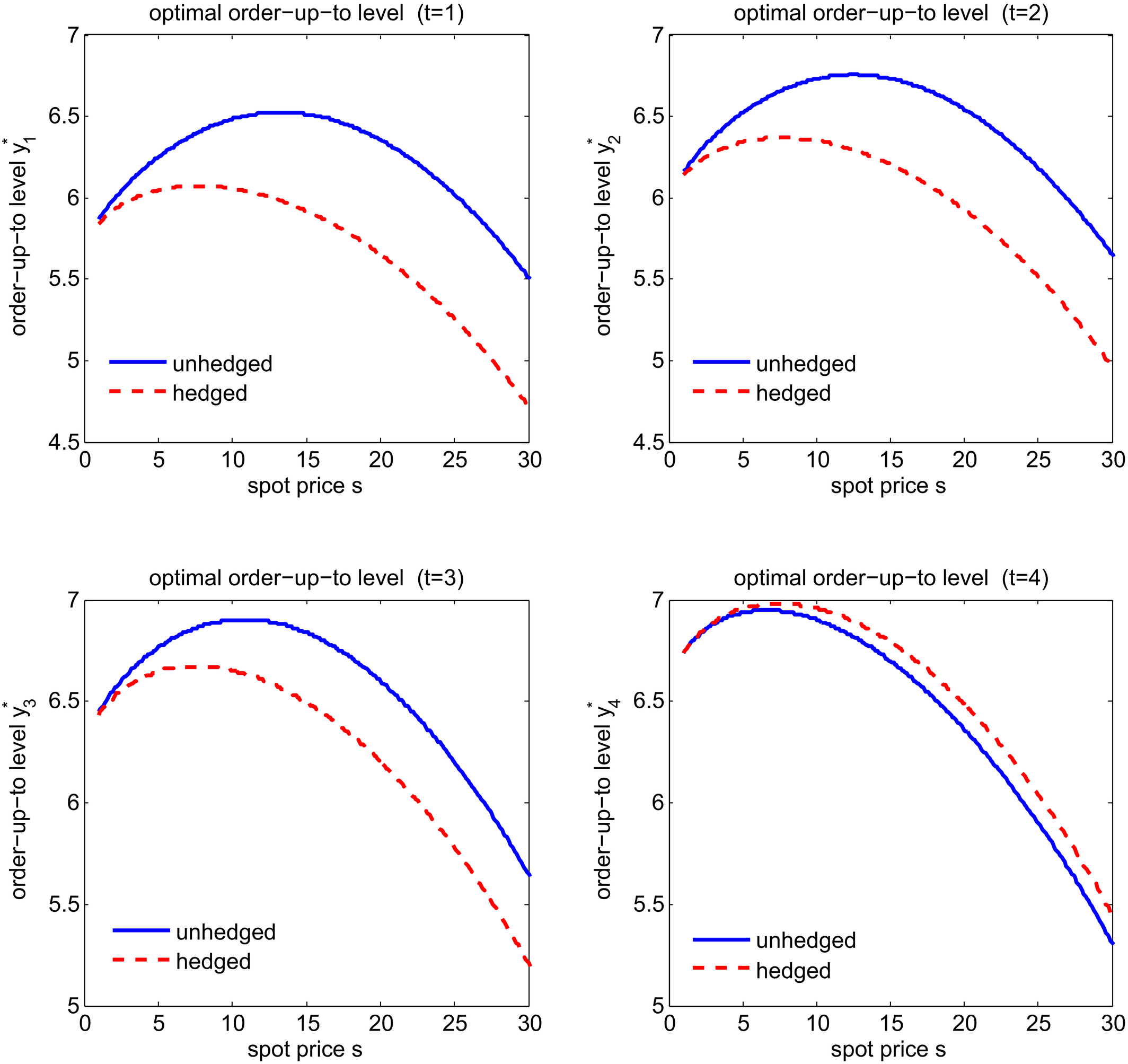
Figure 2 demonstrates the structure of hedging strategies. Note that the positive (negative) sign indicates a long (short) position. In the last period, the optimal hedging policy should offset the risk associated with the carryover inventory, which implies a short position. Hence the sign is negative. But in the previous period, the hedging positions are all positive, which echoes the preceding analysis that the negative correlation between the spot price S _t+1 and profit‐to‐go v _t(S _t+1) may drive the firm to enter a long position. Moreover, the firm will buy (long) more forwards in earlier period than that in later periods. Under the exotic hedges, the firm tends to enter short positions in call options in the earlier periods and long positions in the later periods, which reveals an opposite pattern to the corresponding forward hedges. Note that the short positions may be due to the convexity of the profit‐to‐go functions and the role of options hedges to offset the convexity. Compared to the optimal forward positions, the numbers of options are relatively smaller, which is driven by the fact that the profit‐to‐go functions decrease almost linearly.

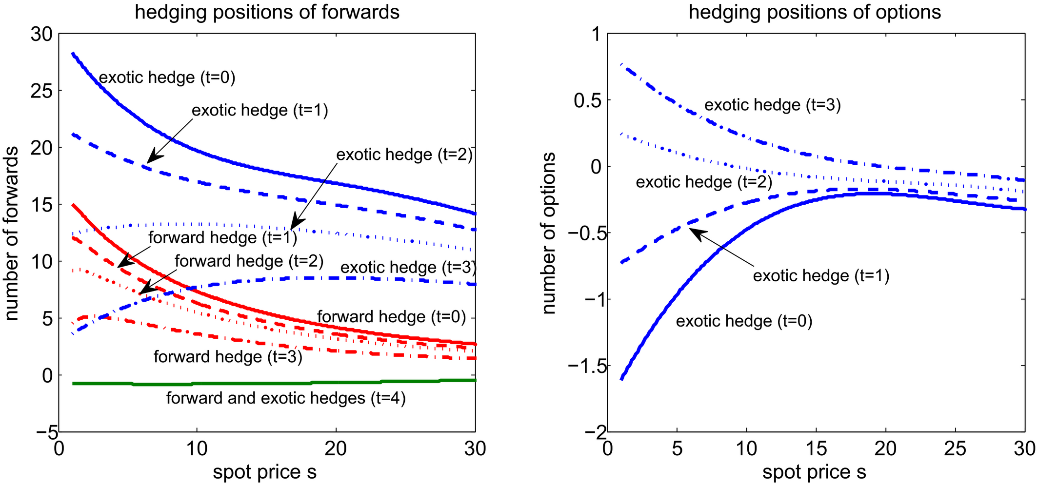
Finally, we compare the means and variances of terminal wealth in different hedging environments. Figure 3 demonstrates the mean and variance performance for periods 0, 2, and 4. The left panels of Figure 3 show that the profit function is decreasing in spot price. The profits under forward hedge and exotic hedge are identical. In the last period, the hedged profit is slightly higher than the unhedged one, but the opposite is observed in the previous periods. This is because the order‐up‐to level under financial hedges in the last period is higher (and thus the profit is closer to the risk neutral one) but in the earlier periods the order‐up‐to levels under financial hedges are lower resulting in lower profits. Also observe that the difference between the hedged and unhedged profits is enlarged when there are more remaining periods, which implies that the value of financial hedging increases in the length of the remaining decision horizon. The right panels of Figure 3 show that in periods 0 and 1 the unhedged variances are greater than that under forward hedge and the later are greater than that under exotic hedge. In the last period, the forward hedge and exotic hedge have the same variance and the unhedged variance is smaller than the hedged variances.

Concluding Remarks

This study addresses a joint inventory and financial hedging decision problem in a dynamic mean‐variance framework for a commodity inventory system with lost sales. Recognizing the time‐inconsistency of mean‐variance criteria, we employ the dynamic programming approach to derive a time‐consistent policy. We characterize the structures of the time‐consistent policies under forward hedge and exotic hedges and compare them to the system in the absence of financial hedges. We show that as long as forward contracts are used the inventory decisions can be separated from the financial hedging decisions and myopic base‐stock policies are optimal. We also show that under exotic hedge the time‐consistent policy is indeed optimal for the original objective of maximizing mean‐variance of terminal wealth over the whole planning horizon in the initial period. Furthermore, we identify conditions under which financial hedges may lead to lower order‐up‐to levels, as contrast to the prediction of the typical one‐period models in the literature that financial hedges may lead to lower order‐up‐to level. We also compare the key financial performance indicators in different hedging environments analytically and examine our results numerically.

Our results shed new light into commodity risk management. Firstly, operational (inventory) decisions and financial hedging decisions interplay with each other. On the one hand, financial hedges allow us to decompose a dynamic inventory decision problem into a sequence of myopic decision problems, which significantly simplifies the inventory decision process. On the other hand, financial hedging decisions rely on inventory strategies, since the future cash flow depends on the inventory policies. In the corporate world, the operational and financial decisions are often made separately, partially because of the difficulty in coordinating the decisions between operational and financial managers. Our model suggests that the operational managers can still enjoy their independence (from the details of the financial decisions) while financial managers to effectively hedge need to better understand the cash flow implications of operational strategies. Secondly, financial hedges can be substitutes to inventories. In the one‐period setting, it is known that the financial hedges and inventory levels are complementary. However, in the earlier periods of a dynamic system, financial hedges may lead to lower inventory levels. That is, in the absence of financial hedges, a firm tends to order more inventory in anticipation of a higher price of purchased materials in the future. Our finding suggests that financial derivatives are better instruments to hedge the future price risk, while the inventory decisions focus on the current demand (quantity) risk which cannot be hedged by financial instruments.

Our model assumes that the financial derivatives are fairly priced so that no profit or loss is expected from financial hedging, which is common in the literature (see, e.g., Chod et al. 2010, Froot et al. 1993, Gaur and Seshadri 2005). In the real world, it is possible that there are non‐zero expected returns from the derivative trading (i.e., E _t[H _t(S _t+1)] ≠ 0), which provides a speculative motive, in addition to the hedging motive, for the firm to use financial derivatives. In this case, using a similar dynamic programming approach, we can also develop a time‐consistent policy which allows us to separate the inventory decisions and financial hedging decisions in the presence of forward hedges. However, it is notable that the time‐consistent policy under the exotic hedge is no longer optimal for the initial objective in problem 4.

A limitation of our model is to assume that the firm has access to capital markets for borrowing and lending any amount of cash with the risk‐free interest rate without concerning bankruptcy or other financial distress costs. Although such an assumption is common in the literature for the sake of analytical tractability, addressing those market imperfections will lead to a more practical model (see e.g., Kouvelis and Zhao 2012), which will be addressed in our future research.

Footnotes

A. Proofs of Statements

Acknowledgments

This research of the second author is partly supported by National Science Foundation of China (NSFC) Grants 71671085 and 71528003, and a RGC Grant from the Research Grants Council of Hong Kong, China (Project No. CityU 11501917). This research of the third author is partially supported by NSFC Grants 71620107002 and 71771100. The authors would like to thank Professor George Shanthikumar, the department editor, the senior editor and two anonymous referees for their constructive comments.

References

Agrawal

Seshadri

. 2000. Impact of uncertainty and risk aversion on price and order quantity in the newsvendor problem. Manuf. Serv. Oper. Manag. 2(4): 410–423.

Back

2017. Asset Pricing and Portfolio Choice Theory, 2nd edn. Oxford University Press, New York.

Basak

Chabakauri

. 2010. Dynamic mean‐variance asset allocation. Rev. Finan. Stud. 23(8): 2970–3016.

Basak

Chabakauri

. 2012. Dynamic hedging in incomplete markets: A simple solution. Rev. Finan. Stud. 25(6): 1845–1896.

Bouakiz

Sobel

M. J.

. 1992. Inventory control with an exponential utility criterion. Oper. Res. 40: 603–608.

Briys

Bellalah

Mai

H. M.

Varenne

F. D.

. 1998. Options, Futures, and Exotic Derivatives: Theory, Application, and Practice. John Willey & Sons, New York.

Brown

G. W.

Toft

K. B.

. 2002. How firms should hedge. Rev. Finan. Stud. 14: 1283–1324.

Caplin

Leahy

. 2006. The recursive approach to time inconsistency. J. Econ. Theory 131: 134–156.

Carr

Madan

. 2001. Optimal positioning in derivative securities. Quant. Finance 1(1): 19–37.

10.

Chen

Sim

Simchi‐Levi

Sun

. 2007. Risk aversion in inventory management. Oper. Res. 55(5): 828–842.

11.

Chod

Rudi

Van Mieghem

J. A.

. 2010. Operational flexibility and financial hedging: Complements or substiutes. Management Sci. 56(6): 1030–1045.

12.

Cui

Shi

. 2017. Self‐coordination in time inconsistent stochastic decision problems: A planner‐doer game framework. J. Econ. Dyn. Control 75: 91–113.

13.

Ding

Dong

Kouvelis

. 2007. On the integration of production and financial hedging decisions in global markets. Oper. Res. 55(3): 470–489.

14.

Duffie

Richardson

H. R.

. 1991. Mean‐variance hedging in continuous time. Ann. Appl. Probab. 1: 1–15.

15.

Eeckhoudt

Gollier

Schlesinger

. 1995. The risk‐averse (and prudent) newsboy. Management Sci. 41(5): 786–794.

16.

Eydeland

Wolyniec

. 2002. Energy and Power Risk Management: New Developments in Modeling, Pricing, and Hedging. John Wiley and Sons, New York.

17.

Froot

K. A.

Scharfstein

D. S.

Stein

J. C.

. 1993. Risk management: Coordinating corporate investment and financing policies. J. Finance 48(5): 1629–1658.

18.

Gaur

Seshadri

. 2005. Hedging inventory risk through market instruments. Manuf. Serv. Oper. Manag. 7(2): 103–120.

19.

Geman

Ohana

. 2008. Time‐consistency in managing a commodity portfolio: A dynamic risk measure approach. J. Bank. Finance 32: 1991–2005.

20.

Hull

J. C.

2008. Options, Futures and Other Derivatives, 7th edn. Prentice Hall, London.

21.

Kleindorfer

P. R.

2009. Integrating physical and financial risk management in supply management. Geman

, ed. Risk Management in Commodity Markets: From Shipping to Agriculturals and Energy. John Wiley & Sons, Chichester, West Sussex, UK, 33–50.

22.

Kouvelis

Zhao

. 2012. Financing the newsvendor: Supplier vs. bank, and the structure of optimal trade credit contracts. Oper. Res. 60(3): 566‐580.

23.

Kouvelis

Ding

. 2013. Managing storable commodity risks: Role of inventories and financial hedges. Manuf. Serv. Oper. Manag. 15(3): 507–521.

24.

Levy

. 2004. Prospect theory and mean‐variance analysis. Rev. Finan. Stud. 17(4): 1015–1041.

25.

W. L.

. 2000. Optimal dynamic portfolio selection: Multiperiod mean‐variance formulation. Math. Finance 10: 387–406.

26.

Markowitz

H. M.

1952. Portfolio selection. J. Finance 7: 77–91.

27.

Markowitz

H. M.

1959. Portfolio Selection: Efficient Diversification of Investments. Wiley, New York.

28.

Markowitz

H. M.

1991. Foundations of portfolio theory. J. Finance 46(2): 496–447.

29.

Martínez‐de‐Albéniz

Simchi‐Levi

. 2006. Mean‐variance trade‐offs in supply contracts. Nav. Res. Log. 53: 603–616.

30.

Miller

M. H.

1997. Merton Miller on Derivatives. Wiley, New York.

31.

Nagali

Hwang

Sanghera

Gaskins

Pridgen

Thurston

Mackenroth

Branvold

Scholler

Shoemaker

. 2008. Procurement risk management (PRM) at HP. Interfaces 38(1): 51–60.

32.

PricewaterhouseCoopers . 2009. Navigation: Managing commdity price risk through market uncertainty. Available at http://www.pwc.com/gx/en/metals/pdf/managing-commodityrisk.pdf (accessed date February 23, 2018).

33.

Routledge

B. R.

Seppi

D. J.

Spatt

C. S.

. 2000. Equilibrium forward curves for commodities. J. Finance 55(3): 1297–1338.

34.

Rudin

1987. Real and Complex Analysis, 3rd edn. McGraw Hill, New York.

35.

Sanda

G. E.

Olsen

E. T.

Fleten

S.‐E.

. 2013. Selective hedging in hydro‐based electricity companies. Energy Econ. 40: 326–338.

36.

Schwartz

E. S.

1997. The stochastic behavior of commodity prices: Implications for valuation and hedging. J. Finance 52(3): 923–973.

37.

Smith

J. E.

Nau

R. F.

. 1995. Valuing risky projects: Option pricing theory and decision analysis. Management Sci. 51(3): 452–466.

38.

Smith

Stulz

. 1985. Determinants of firms hedging policies. J. Finan. Quant. Anal. 20: 391–405.

39.

Strotz

R. H.

1956. Myopia and inconsistency in dynamic utility maximization. Rev. Econ. Stud. 23: 165–180.

40.

Topkis

D. M.

1998. Supermodularity and Complementarity. Princeton University Press, Princeton, NJ.

41.

Turcic

Kouvelis

Bolandifar

. 2015. Hedging commodity procurement in a bilateral supply chain. Manuf. Serv. Oper. Manag. 17(2): 221–235.

42.

Weiss

2005. A Course in Probability. Addison‐Welsley, Boston.

43.

Williams

J. C.

Wright

B. D.

. 1991. Storage and Commodity Markets. Cambridge Unversity Press, Cambridge.

44.

Working

1948. The theory of the price of storage. Am. Econ. Rev. 39: 1254–1262.