
Abstract
We consider a periodic review, joint inventory and pricing control problem for a firm that faces general random price‐dependent demands. Any unsatisfied demand can be either backordered or lost immediately. The objective is to maximize the expected profit over a finite selling horizon by coordinating the inventory and pricing decisions in each period. For both the backorder model and the lost sales model, we derive some quite general sufficient conditions to ensure the optimality of a base‐stock list price (BSLP) policy based on the strict monotonicity of demand functions in the realizations of random noises. We are among the first to utilize the strict monotonicity of demand functions in the realizations of random noises for deriving the sufficient conditions. We derive the sufficient conditions in both the backorder model and the lost‐sales model by utilizing the new concept of upper‐set and lower‐set decreasing properties (USDP/LSDP), which is a generalized version of the first‐order stochastic dominance. This study reveals that the optimality of a BSLP policy is robust to more general business environments than what we previously thought. Finally, we also apply the USDP/LSDP in other inventory management problems.
Introduction
Pricing strategies become increasingly important in retail and manufacturing sectors due to the development of information technology. Firms can easily change their prices based on demand seasonality, inventory levels, and production schedules, etc. In practice, the inventory‐based dynamic pricing is adopted by firms like Dell, Amazon, FairMarket, Land's End, and J.C. Penney (Chan et al. 2004, Elmaghraby and Keskinocak 2003). Through coordinating inventory and pricing strategies, significant benefits can be reaped for these firms (Chen and Simchi‐Levi 2012).
To be implementable in practice, a joint inventory and pricing strategy is required to have a simple structure. An appealing candidate is the so‐called base‐stock list price (BSLP) policy. Under this policy, there is a base‐stock level. Whenever the inventory level is below the base‐stock level, the firm orders up to that level and charges a list price. Otherwise, no order is placed and the price is decreasing in the inventory level. However, this simple policy may not always be optimal. To ensure the effectiveness of a BSLP policy, it is thus critical to identify conditions and business environments under which a BSLP policy is optimal. The optimality conditions provide valuable benchmarks for the implementation of a BSLP policy in practice.
The joint inventory and pricing control has received considerable attention over the past ten years. Validating the optimality of a BSLP policy is one of the focuses in the existing literature. However, the existing literature suffers the following two limitations: (i) for the backorder setting, it requires unnecessarily restrictive functional forms of demand; (ii) the lost‐sales setting is suitable for describing the business model of retail, but its corresponding results are very limited and hence this setting remains largely unknown. Specifically, for the backorder setting, there are mainly three classes of demand functions considered in the existing literature: additive functions, multiplicative functions and generalized additive functions. Beyond these three classes, our understanding is very limited for the optimality of a BSLP policy. Under the lost‐sales setting, in the existing literature, we do not know when a BSLP policy is optimal in a finite selling horizon even under the additive demand functions due to its technical challenges, not to mention the general demand functions. This raises doubts on the applicability of a BSLP policy in practice.
The two limitations mentioned above mainly result from the technical challenges caused by the general demand functions and the revenue function in the lost‐sales setting. More specifically, with the general demand functions, it is challenging to show the joint concavity of the single‐period expected profit function under the backorder setting because the composition of two concave functions in general is not concave. For the lost‐sales setting, the revenue function in each period is censored by the inventory level, and as a result it may not be concave. To overcome these technical challenges, we utilize the monotonicity of demand functions in the realizations of random noises.
The focus of our study is to identify the conditions for the optimality of a BSLP policy under a finite selling horizon with general demand functions. We do not impose any particular form on how demand depends on price and random noise. Consistent with the existing inventory‐pricing literature, we consider two classical inventory models: the backorder inventory model and the lost‐sales inventory model with a single stage and zero leadtime. By adopting the monotonicity of demand functions introduced above, we are able to identify sufficient conditions to ensure the optimality of a BSLP policy under general demand functions.
Specifically, we show for the backorder setting that a BSLP policy is optimal in each period if demand functions are decreasing in price and strictly decreasing (increasing) in the realizations of random noises, and their sensitivities in price have the upper‐set (lower‐set) decreasing property (USDP/LSDP). The new concept of USDP/LSDP is in fact a generalized version of the first‐order stochastic dominance. The demand sensitivity in price has the LSDP (USDP) if it is stochastically increasing (decreasing) in price. If a demand function is concave in price, then its sensitivity in price must have the USDP and LSDP. However, the concavity or convexity in price is not necessary to ensure the USDP/LSDP.
For the lost‐sales setting, we show that a BSLP policy is optimal in each period if (i) demand functions are decreasing in price and strictly decreasing (increasing) in the realizations of random noises, and their sensitivities in price have the USDP (LSDP), and (ii) the single‐period expected profit function is submodular in price and inventory level. Under the single‐period setting, Kocabiyikoğlu and Popescu (2011) show that the sufficient conditions for the optimality of a BSLP policy are that the demand function is decreasing in price and increasing in the realizations of random noises, the riskless unconstrained revenue function is concave in price for any realizations of random noises, and the single‐period expected profit function is submodular in price and inventory level. We show that, unlike the single‐period setting, we require the USDP/LSDP of the sensitivity of demand functions in price in the multi‐period setting, which also guarantees the concavity of the expected riskless unconstrained revenue function in price. We do not require that the revenue function is concave in price for any realizations of random noises. In summary, in spite of the technical challenges, we find that a BSLP policy is optimal for both the backorder inventory model and the lost‐sales inventory model under quite general conditions.
The proposed concept of USDP/LSDP can be applied to other operations management problems. We show for example in both the backorder model and the lost‐sales model, with inventory‐dependent demands, the USDP/LSDP can be used to guarantee that an inventory‐dependent base‐stock policy is optimal; with quality‐dependent demands, the USDP/LSDP can lead to the optimality of the base‐stock list quality level policy.
In summary, our contributions include the following: We consider general price‐dependent demands in a multi‐period setting and show that a BSLP policy is optimal under more general sufficient conditions compared with the conditions proposed in the existing literature for both the backorder model and the lost‐sales model. We are among the first to derive results by utilizing the strict monotonicity of demand functions in the realizations of random noises. To show the joint concavity of our objective functions in both the backorder model and the lost‐sales model, we propose the concept of USDP/LSDP, show the preservation of its monotonicity under the expectation with a class of monotone functions, and exploit the monotonicity of demand functions in the realizations of random noises. In addition, based on the USDP/LSDP, we show the concavity of a function that is a composite of a concave function with another function having the USDP/USLP.
Related Literature
There is an extensive literature on joint pricing and inventory control strategies starting with Whitin (1955). Whitin (1955) analyzes an EOQ model with deterministic (price‐dependent) demand. On models with stochastic demand, there are two streams of literature: one focuses on single‐period problems and the other focuses on multi‐period problems. See Petruzzi and Dada (1999), Elmaghraby and Keskinocak (2003), Yano and Gilbert (2004), and Chen and Simchi‐Levi (2012) for comprehensive reviews. The early single‐period coordinating inventory and pricing control models include Mills (1959, 1962), Karlin and Carr (1962), Zabel (1970), Young (1978), Cheng (1984), Lau and Lau (1988), and Polatoglu (1991). Recent studies on single‐period models include Yao et al. (2006), Kocabiyikoğlu and Popescu (2011), and Lu and Simchi‐Levi (2013). In particular, Kocabiyikoğlu and Popescu (2011) consider the lost‐sales model in a single‐period setting and provide sufficient conditions to ensure the concavity and submodularity of the objective functions.
One stream of literature focuses on multi‐period models under the backorder setting. Zabel (1972) analyzes both the additive and multiplicative demand functions where the random noise follows a uniform or exponential distribution that is independent of price. Thowsen (1975) extends Zabel's (1972) results for the additive demand function by assuming the random noise follows a Pólya frequency function of order 2 (PF2) distribution and finds that a BSLP policy is optimal. Federgruen and Heching (1999) establish the optimality of a BSLP policy with a general demand function for a backorder system without capacity constraints. Their sufficient conditions are as follows: (i) the demand is decreasing and concave in the list price; (ii) the single‐period expected inventory cost is jointly convex in the order‐up‐to level and price. However, as indicated by the authors themselves and Feng et al. (2013), the joint convexity of the single‐period expected inventory cost function can be guaranteed if the demand function is linear in the price, which is quite restrictive, but easily fails when the demand is a nonlinear function of the price.
Due to the technical challenges caused by the general demand function, the subsequent literature mainly considers the following classes of demand functions: additive demand function, multiplicative demand function, combined additive and multiplicative demand function (Chen and Simchi‐Levi 2004a), and generalized additive demand function (Feng et al. 2013). In fact, both Chen and Simchi‐Levi (2004a) and Feng et al. (2013) consider a mixture of additive and multiplicative demand functions.
Chen and Simchi‐Levi (2004a,b) generalize Federgruen and Heching's (1999) model by incorporating a positive and fixed ordering cost, and relaxing the concave demand assumption. Based on the combined additive and multiplicative demand function, they prove that an (s, S, p) policy is optimal for the additive demand function and an (s, S, A, p) policy is optimal for the combined demand function. Chen et al. (2010), based on the additive demand function, consider the concave ordering cost and show that a generalized (s, S, p) policy is optimal if the random noise in a demand function follows a positive Pólya or uniform distribution. Chen and Zhang (2014) analyze a non‐stationary inventory system with the additive demand function and show that a time‐dependent (s, S, p) policy is optimal.
Feng et al. (2013) consider the generalized additive demand function, which involves the relationship between scale and location parameters. They show that a BSLP policy is optimal under a new set of optimality conditions that depend on the location and scale parameters of the demand. Bernstein et al. (2016) consider both additive and multiplicative demand functions for systems with a positive lead time. They propose a simple heuristic consisting of a myopic pricing policy and a base‐stock policy for replenishment. Lu et al. (2016) assume a combined additive and multiplicative demand function and consider that the demand information is incomplete in reality. By introducing a new concept named K‐approximate convexity, they obtain a base stock list price policy with a good performance. An intriguing research question is: Can we identify general sufficient conditions beyond the aforementioned classes of demand functions to ensure the optimality of a BSLP policy under the backordering setting?
There are only a few studies that consider the multi‐period lost‐sales setting. This is due to the technical difficulty that the demand is censored by the inventory level. For a system with fixed ordering cost and general demand functions, Polatoglu and Sahin (2000) provide some sufficient conditions for an (s, S, p) policy to be optimal. But, as indicated by Chen and Simchi‐Levi (2004a), it is not clear if their conditions can be satisfied by any demand function. For example, a linear demand function does not necessarily match those requirements. When the demand is in the additive form, Chen et al. (2006) establish the optimality of an (s, S, p) policy by imposing some restrictions on the distribution of demand uncertainty as well as some restrictions on the inequality involving expected demand and price. When the demand is in the multiplicative form, Song et al. (2009) demonstrate the optimality of an (s, S, A, p) policy for a finite horizon problem. Furthermore, the optimal policy can be simplified to a base‐stock policy when the fixed ordering cost is zero. For both the lost‐sales model and the backorder model, Huh and Janakiraman (2008) use an alternative approach to investigate the sufficient conditions for the optimality of an (s, S, p) policy based on the combined additive and multiplicative demand function.
Different from the existing literature, to show the optimality of a BSLP policy in a multi‐period setting, we utilize the monotonicity of general demand functions in the realizations of random noises. We are able to derive a set of general sufficient conditions for the lost‐sales setting. A more relax set of sufficient conditions are obtained for the backorder setting.
The remainder of the study is organized as follows. We describe our model settings in section 3 and present some preliminary results in section 4. Section 5 provides formulations and analytical results for the backorder model and the lost‐sales model, respectively. Section 6 discusses some applications of our results and proposed concepts. Finally, we provide concluding remarks in section 7. All proofs and some of the intermediate results are relegated to Appendix S1.
Model Settings
We consider a single‐product single‐stage periodic‐review inventory problem with general price‐dependent demands. The finite selling horizon consists of T periods. The demand in each period only depends on the prevailing list (selling) price, that is, customers are myopic. Following Federgruen and Heching (1999), we assume the demand in period t is


The sequence of events in each period is as follows: (i) at the beginning of each period, an ordering decision and a pricing decision are made simultaneously; (ii) the order in this period arrives; (iii) demand is realized after customers observe the list price; (iv) finally, the revenue/cost is charged at the end of the period. For unfilled demand, we consider either the backorder setting or the lost‐sales setting.
To analyze the inventory‐pricing problems, we impose the following two assumptions on the demand functions.
For all t, t = 1, …, T, (i) the demand function d
t
(p
t
, ζ) is decreasing in p
t
and strictly monotone in ζ, where ζ denotes the realization of


The fact that d t (p t , ζ) is decreasing in p t is a regular assumption on demand functions, that is, as price increases, demand should decrease.
Unlike the existing literature, the monotonicity of d t (p t , ζ) in ζ plays a critical role in our analysis. In fact, under the multiplicative or additive demand models, we already assume some monotone properties for the random noises. However, the monotonicity is not utilized in deriving the structural properties of the optimal profit functions in the existing literature.
Since d
t
(p
t
, ζ) is strictly monotone in ζ, there exists some


We are not the first to assume the thrice continuous differentiability of the demand function. Chen et al. (2006) and Huh and Janakiraman (2008) make similar assumptions to derive sufficient conditions for the optimality of an (s, S) policy under the lost‐sales model. Assumption 2 is needed to ensure the twice continuous differentiability of the expected discounted profit functions in the backorder and the lost‐sales models. We denote by
Based on the model setting discussed above, we then introduce a new concept and present some preliminary results that shall be used to derive our main results.
Preliminary Results
To empower our analysis, we introduce the notion of upper‐set (lower‐set) decreasing property as follows.
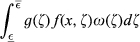
A function f(x, ϵ), where ϵ is a random variable with the density function ω(·) and

The USDP/LSDP is similar to the first‐order stochastic dominance for random variables. However, f(x, ϵ) may not be a density function as it might be negative.
Note that if f(x, ϵ) is decreasing in x for any realization of ϵ, then it must have the USDP/LSDP. But a function f(x, ϵ) having the USDP/LSDP is not necessarily decreasing in x for any ϵ. To illustrate this point, we provide an example of USDP as follows:
Let f(x, ϵ) = x
ϵ
ln (x), where ϵ is uniformly distributed over [1, M] and 0 ≤ x ≤ e
− ln (M)/(M − 1). Then, f(x, ϵ) is not always decreasing in x for any realization of ϵ. Instead, f(x, ϵ) is decreasing in x when x → 0 for any ϵ but may be increasing in x when x → e
− ln (M)/(M−1) and the realization of ϵ is small. Note that


A function with the USDP/LSDP leads to the following results.
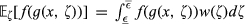
For a continuous random variable ϵ with a density function ω(·), f(x, ϵ) has the USDP if and only if
Lemma 1 shows that the integration in Equation 1 can preserve the monotonicity for any non‐positive and increasing/decreasing function g(·) under certain conditions. This result is new in the existing literature.
Note that f(x, ϵ) is stochastically increasing (decreasing) in x if and only if
Based on Lemma 1, we then show that the USDP/LSDP can also be used to ensure the joint concavity of the expected value of a composite function.
Let
f(·) is a decreasing and concave function;
ψ(z, ζ) is strictly decreasing (increasing) in ζ and ψ
z
(z, ζ) has the USDP (LSDP).
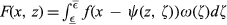
Proposition 1 is critical for the analysis of the backorder and the lost‐sales models. It is worth noting that, in this proposition, we do not require ψ(z, ζ) being concave in z for any ζ to ensure the joint concavity of F(x, z). Proposition 4 is also useful for analyzing operations management models where demand could depend on some other factors, for example, inventory, quality, etc.
Based on Proposition 1, if a single‐variable function f(·) is concave and increasing, then


The Optimality of a BSLP Policy
With the preliminary results above, we now are ready to analyze the backorder model and the lost‐sales model sequentially. For each of the models, we present individually the dynamic programming formulations and the analytical results. For the ease of exposition, we make the following assumption in subsequent analysis.
The demand function


Note that we do not impose any particular class of distributions for

The Backorder Model
In the backorder model, unfulfilled demand in each period is backordered and leftover inventory is carried over to the next period. Given the initial state x
t
, the order quantity q
t
, and the list price p
t
in period t, the state at the beginning of period t+1 transits to


There are a unit backordering cost b for backordered demand and a unit holding cost h for leftover inventory. Then, the single‐period inventory cost incurred in period t is denoted by

Let


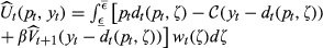
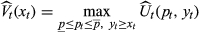
We then shall provide sufficient conditions to ensure that the optimal policy in the backorder model can be described by a BSLP policy, that is, the ordering policy is a base‐stock policy and the price is decreasing in the order‐up‐to level. Essentially, we seek to establish the joint concavity and submodularity in the order‐up‐to level and the list price for the objective function


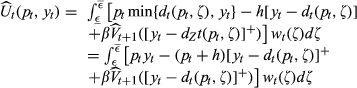
To facilitate our analysis for the backorder model, we first make an equivalent transformation to the dynamic recursion of this problem as follows:
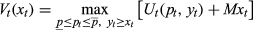
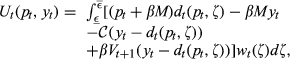


The equivalent transformation of dynamic recursion is critical in deriving sufficient conditions for the optimality of a BSLP policy in the backorder model. Without this transformation, it would be difficult to investigate the joint concavity of

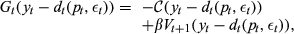
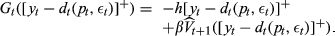
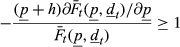
We then present the sufficient condition for the submodularity of


Suppose that V
t+1(·) is continuously differentiable and concave, then


Lemma 2 indicates that the submodularity of the value function


Lemma 2 also reveals our motivation of applying the equivalent transformation for the dynamic recursion of the backorder model as in Equation 4. We make the transformation in order to find the condition under which the function G
t
(·) is monotone. The monotonicity of G
t
(·) plays a critical role in ensuring the joint concavity of

Note that, if p
t
< b, the firm is better off by rejecting the demand when there is no inventory on hand to avoid the additional cost b − p
t
. In this case, a lost‐sales model may be more appropriate. Therefore, in this backorder model, we consider p
t
≥ b or equivalently
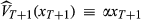
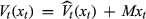
Based on Lemma 2 and the fact that

Suppose M = −b/β and
V
t
(x
t
) is continuously differentiable and
V
t
(x
t
) is concave in x
t
, The optimal policy can be described by a BSLP policy: In each period t, there exist a unique base‐stock level


In Theorem 1, the condition that


To derive the sufficient condition for the optimality of a BSLP policy in the backorder model, we set M = −b/β in this theorem due to the following reason. The monotonicity of G
t
(·) in Equation 6 and the concavity of


Recall that if f(x,ϵ) is stochastically increasing (decreasing) in x, then it must have the LSDP (USDP) (see Remark 4). Hence, if


In addition to the stochastically increasing/decreasing functions, most of the existing demand models have the USDP/LSDP. When


Demand Models that Have the USDP/LSDP
The Lost‐Sales Model
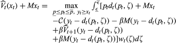
In the lost‐sales model, in each period, any unfilled demand is lost immediately and leftover inventory is carried over to the next period. Given the order‐up‐to level 
There are a unit holding cost h for leftover inventory and a discount factor β ∈ [0, 1]. Different from the traditional inventory models without explicitly stating selling prices, under our setting, we do not charge additional lost‐sales cost since the lost opportunity cost has been reflected in the revenue function 


Let 


For the ease of exposition, we aggregate the functions depending on 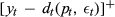

We then provide the sufficient conditions for the optimality of a BSLP policy in the lost‐sales model. We adopt the similar analytical approach as in the backorder model. However, in the lost‐sales model, the demand is censored by the inventory level, which makes the problem more challenging than the backorder model. For example, 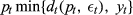

We tackle the joint concavity of the profit function 

Suppose that
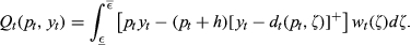
The single‐period expected profit function 


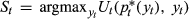
Based on Lemma 3, we then provide sufficient conditions in the following theorem for the optimality of a BSLP policy in the lost‐sales model. Note that, to show the optimality of a BSLP policy, it is sufficient to show that 

Under the following conditions:
the single‐period expected profit function for t = 1, …, T, we have the following results:
The optimal policy can be described by a BSLP policy: in each period t, there exist a unique base‐stock level


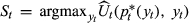
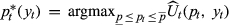


Two sufficient conditions are required for the optimality of a BSLP policy in the multi‐period setting. Similar to the sufficient condition in Theorem 1 for the backorder model, the condition (i) in Theorem 2can be equivalently claimed as that 


Under Assumption 3, the single‐period expected profit function 


Proposition 2 indicates that the inequality 12 is the sufficient and necessary condition to ensure the submodularity of the single‐period expected profit function 
In fact, when h = 0, Proposition 2 is essentially the same as the proposition 1 in Kocabiyikoğlu and Popescu (2011). 

Similar to Kocabiyikoğlu and Popescu (2011), under certain conditions, the monotonicity of 

If 


When 


Suppose that, in each period t, there is a nonnegative minimum demand quantity denoted by 


We then illustrate some demand functions, as well as their corresponding conditions, under which the two sufficient conditions in Theorem 2 for the optimality of a BSLP policy can be guaranteed. Recall that 


Suppose that W
t
has the IFR property and there is a non‐negative minimum demand denoted by Under an additive demand function Under a multiplicative demand function Under a generalized additive demand function Under a logarithmic demand function 


Corollary 1 follows directly from the condition in Equation 12 and the IFR property. The IFR property holds for most well‐known distributions, for example, uniform, normal, truncated‐normal, logistic, log‐normal, exponential, Laplace, Weibull distributions, etc.
In Corollary 1, we only illustrate the demand functions that are increasing in the random noise 


Discussions
In this section, we present some discussions for the results in the backorder model and the lost‐sales model sequentially. For the backorder model, the strict monotonicity of the demand function w.r.t the realizations of random noises plays an important role in deriving its results in Theorem 1. In Federgruen and Heching (1999), to ensure the joint concavity and submodularity of the value function for the backorder model, they require that (1) 


In the backorder model, Feng et al. (2013) provide a set of conditions to ensure the optimality of a BSLP policy under the generalized additive demand function 
Sufficient Conditions under the Generalized Additive Demand Function 
For the lost‐sales model, Kocabiyikoğlu and Popescu (2011) have investigated the optimality of a BSLP policy in a single‐period setting with general price‐dependent demands. They show that it is challenging to derive the sufficient conditions even in the single‐period problem. However, as stated by Feng et al. (2013), the approach used by Kocabiyikoğlu and Popescu (2011) is not helpful to tackle multi‐period models as the technique needed for multi‐period models can be fundamentally different from that for single‐period problems. This is because that, in general, 


In the single‐period setting, Kocabiyikoğlu and Popescu (2011) provide the following sufficient conditions for the optimality of a BSLP policy when h = 0: (a) 


Extensions
In this section, to show the applications of USDP/LSDP, we analyze inventory management problems with inventory‐dependent demands and quality‐dependent demands. Similar to the basic model with price‐dependent demands, the USDP/LSDP serves as a more general condition, compared with the restrictive sufficient conditions in the existing literature, that leads to the (joint) concavity of the value functions for the two problems discussed below.
Inventory Management with Inventory‐Dependent Demands
There is a widely recognized phenomenon in marketing that the demand of many retail items is affected by the amount of inventory displayed, e.g., the scarcity effect. We refer to such kind of demand as the inventory‐dependent demand.
The inventory‐dependent demand has been considered by, e.g., Yang and Zhang (2014) and Smith and Agrawal (2017) in the existing literature. Sapra et al. (2010) consider inventory management with a multiplicative form of inventory‐dependent demand under the backorder setting. Following Sapra et al. (2010), we assume that the demand is decreasing in the ending inventory in the previous period but we consider a general demand model. We denote by 
We denote by V
t
(x
t
) the expected optimal discounted cost function from period t and onward, and 

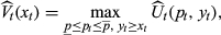
Let M = −b/β. For t = 1, …, T, if
V
t
(x
t
) is concave and An inventory‐dependent base‐stock policy is optimal: there exists


Similarly, for the lost‐sales model, we have the following results.
For t = 1, …, T, if
V
t
(x
t
) is concave and An inventory‐dependent base‐stock policy is optimal: there exists
The Lost‐sales Model


Inventory Management with Quality‐Dependent Demands
In practice, firms may order semi‐products and then make the end‐products once the demands are realized, for example, the postponement strategy of mass customization, so that they can control the quality level of the end‐products. It is well known that the demand is induced by quality in the marketing literature. In each period, the firm first announces the quality level of end‐products, denoted by 


We denote by V
t
(x
t
) the expected optimal discounted cost function from period t and onward, 

Let M = −b/β. For t = 1, …, T, if
V
t
(x
t
) is concave and A base‐stock list quality level policy is optimal: there exist a unique base‐stock level The Backorder Model


Similarly, for the lost‐sales model, we have the following results.
For t = 1, …, T, if
V
t
(x
t
) is concave and A base‐stock list quality level policy is optimal: there exist a base‐stock level S
t
and an optimal list quality level The Lost‐Sales Model


Concluding Remarks
The joint inventory and pricing control has received considerable attention in the literature. For the validation of the optimality of a BSLP policy, the existing literature suffers two limitations: for the backorder setting, it requires unnecessarily restrictive functional forms of demand while the results for the lost‐sales setting are very limited, especially for the multi‐period setting. This may cast doubts over the applicability of the BSLP policy in practice.
To overcome these two limitations, we utilize the monotonicity of the demand functions in the realizations of random noises to derive structural properties of the value functions. Based on such a monotone property, for the backorder model, we show that a BSLP policy is optimal in each period if demand functions are decreasing in price and strictly decreasing (increasing) in the realizations of random noises, and their sensitivities in price have the USDP (LSDP), where USDP/LSDP is a generalized version of the first‐order stochastic dominance. For the lost‐sales model, we show a BSLP policy is optimal if demand functions are decreasing in price and strictly decreasing (increasing) in the realizations of random noises, their sensitivities in price have the USDP (LSDP), and the single‐period expected profit function is submodular in price and inventory level.
Our results can be generalized to systems with Markov modulated demand under similar conditions. For Markov modulated demand, under similar conditions, we can show that a state‐dependent BSLP policy is optimal, where the state refers to the Markov modulating state. Through the above discussion, we show that the optimality of a BSLP policy is robust to more general business environments than what we previously thought. We also apply the USDP/LSDP in other operations management models where demand could depend on other factors, for example, quality and inventory.
In our settings, we assume that all unsatisfied demands are either backordered or lost immediately. It is interesting to generalize our results to the cases with partial backorder and partial lost‐sales. This may be possible since we show that if demand functions are decreasing and concave in price and are strictly monotone in the realizations of random noises, then a BSLP policy is optimal for either the backorder setting or the lost‐sales setting.
Footnotes
Acknowledgments
The authors thank the departmental editor Panos Kouvelis, the senior editor and two anonymous reviewers for their valuable comments and suggestions, which substantially improved the study. The research of Xiaobei Shen was supported by the National Natural Science Foundation of China (grant no. 71701190 and 71731010). The research of Yimin Yu was partially supported by grants from the Research Grants Council of the Hong Kong Special Administrative Region, China (grant no. GRF 11506015, T32‐102/14‐N and T32‐101/15‐R) and CityU 7005014.