The Impact of Valuation Heterogeneity on Equilibrium Prices in Supply Chain Networks

Abstract

This paper studies bargaining in two‐sided supply chain networks where manufacturers on the demand side purchase an input from suppliers on the supply side. The manufacturers may have heterogeneous valuations on the input sold by the suppliers. In such a supply chain network, a manufacturer and a supplier must have a business relationship or “link” to bargain and trade with each other. However, a firm on one side of the supply chain network might not have a business relationship with every firm on the other side of the supply chain network. We show that valuation heterogeneity, supply and demand balance, and network structure are the main factors that influence the equilibrium prices, trading pattern, and surplus allocation in such a supply chain network. Valuation heterogeneity among manufacturers can mitigate unfavorable supply and demand balance to protect some surplus for the manufacturers and leads to higher price dispersion in the supply chain network. We demonstrate that bargaining effectively takes place in smaller subnetworks in a general supply chain network and develop an algorithm to decompose the general network into these smaller subnetworks, which simplifies the analysis of the general supply chain network significantly. We then identify types of supply chain networks that are efficient so that only manufacturers with the highest valuations are able to trade and types of links that can be added into a supply chain network to improve its efficiency.

Keywords

supply chain network competitive bargaining supply chain efficiency

Introduction

This study considers two‐sided supply chain networks where manufacturers on the demand side purchase an intermediate input or component (e.g., DRAM chips) for their final products (e.g., tablets and/or smart phones) from suppliers on the supply side. A manufacturer and a supplier in such a supply chain network must have a business relationship or “link” to bargain and trade with each other. However, a manufacturer may not have a business relationship with every supplier in the supply chain network. Lacking a business relationship between two firms can be caused by various factors such as transportation costs, geopolitical restrictions, technological compatibility, social contacts [among managers], etc. (Jackson 2008). The pattern of the business relationships between manufacturers and suppliers in a supply chain forms the network structure of the supply chain. The network structure of a supply chain restricts and influences competition, and therefore the possible trading outcomes in the supply chain network. Two firms on different sides of a supply chain network cannot trade if they have no business relationship with each other. Firms on one side of a supply chain network may need to compete for the trade with a firm on the other side of the network they all have a business relationship with.

Although they are buyers of a common input in a supply chain network, manufacturers can be different from each other. First, their final products can be different: The end products could be totally different products or they could be similar products that have different values and margins and target different segments or markets. As a result, the manufacturers’ valuations (or willingness to pay) on the component are different. Second, the manufacturers’ business relationships with the suppliers in the network could be different too. The manufacturers may have business relationships with different suppliers in the network and some of them have business relationships with more suppliers than others do. In the presence of these differences in such a supply chain network, many interesting questions, from both firms’ perspectives and the whole supply chain network's perspective arise. How should a manufacturer in a supply chain network bargain with suppliers who have a business relationship with her to secure the supply of the component for her final products at a good price? How should a supplier respond to offers from manufacturers? When market clears, what does the final trading outcome of the network look like, that is, who will trade with whom in the network at what prices? Is the final trading outcome efficient so that only manufacturers with the highest valuations on the component are able to trade? How can the efficiency of a supply chain network be improved? This study aims to answer these questions.

We model a two‐sided supply chain network via a bipartite graph. The nodes in the bipartite graph represent firms: The manufacturers are on one side and the suppliers are on the other side of the bipartite graph. A link between two firms on different sides of the graph represents that the two firms have a business relationship and can bargain and trade with each other. The manufacturers have different valuations on the component. To facilitate tractability, we assume that each manufacturer purchases only one unit of the component and each supplier can supply only one unit of the component. Therefore, in the supply chain network, one manufacturer and one supplier can form a match with balanced supply and demand of the component. The manufacturers bargain with the suppliers on the prices of the component following a generalized version of Rubinstein (1982) bargaining model where bargaining occurs in an alternating order between the manufacturers and the suppliers. Firms will keep bargaining by proposing and responding to offers in alternating orders until all firms trade or no possible trades can be made because there are no links left. With this model of supply chain network, we establish the following main findings.

First, we show that valuation heterogeneity among manufacturers plays an important role in interacting with supply and demand balance and network structure of a supply chain network to influence the equilibrium outcome of the supply chain network. Existing literature (e.g., Corominas‐Bosch 2004) has shown that if there are more manufacturers than suppliers (i.e., there is a supply shortage and manufacturers need to compete for limited supplies) and the manufacturers have the same valuation, the suppliers would be able to take advantage of the competition among the manufacturers to push the prices all the way up to their homogenous valuation. As a result, the suppliers capture all the surpluses of the trades while the manufacturers get zero surplus. However, we find that this is no longer the case when the manufacturers have heterogenous valuations. Now, the suppliers cannot simply push the prices to a uniform level to capture all surpluses of the trades anymore because the manufacturers are now differentiated from each other in their valuations. Therefore, valuation heterogeneity serves as a counter force to unfavorable supply and demand imbalance to protect the manufacturers from price hikes and surplus extractions by the suppliers. Furthermore, when manufacturers have heterogeneous valuations, suppliers prefer to trade with manufacturers with high valuations because they can potentially pay more. In other words, suppliers have stronger preferences over whom to trade with than they do when manufacturers have the same valuation. This increased preference leads to more prices or price dispersion in a supply chain network because the exact price a supplier can get from a trade critically depends on the exact valuation of the manufacturer involved in the trade.

Second, we find that bargaining actually takes place in smaller subnetworks in a general supply chain network because firms may selectively bargain with a subset of firms with whom they are linked. In other words, firms may strategically ignore some of their links in the network that are not useful for them to get a better deal. We show that any supply chain network can be decomposed into a union of three types of subnetworks. In each of these three types of subnetwork, the equilibrium prices of all trades are determined jointly by manufacturer valuations, supply and demand balance, and network structure in the subnetwork independent of the rest of the network. With this decomposition result, we can simplify the analysis of a general supply chain network significantly to determine the equilibrium outcome of the network.

Third, we identify what types of supply chain networks are efficient. When manufacturers have different valuations, efficiency of a supply chain network becomes a concern. In an efficient supply chain network, only the manufacturers with the highest valuations can trade so the total surpluses of all trades are maximized (which is not a concern when all manufacturers have the same valuation). For a supply chain network to be efficient, we find that manufacturers with high valuations must be well connected. Then, we identify the types of links to add into a supply chain network to improve the efficiency of the network. Adding a new link into a supply chain network can improve its efficiency if with the new link more trades can happen in the network or manufacturers with higher valuations can replace manufacturers with lower valuations to trade in the network. Therefore, an efficiency improving link must connect to a manufacturer, especially with a high valuation, in a subnetwork with more manufacturers than suppliers where the manufacturers need to compete for limited supply. With this new link, the manufacturer can potentially reach out to a new source of supply outside of the subnetwork to either make a new trade possible or replace a manufacturer with lower valuation to trade to improve the efficiency of the supply chain network.

Literature Review

Existing supply chain literature mainly focuses on simple supply chains with limited numbers of firms and specific network structures such as one‐manufacturer‐one‐supplier (e.g., Pasternack 1985, Spengler 1950), one‐manufacturer‐multiple‐suppliers (e.g., Bernstein and Federgruen 2005, Cachon and Lariviere 2005, Feng et al. 2015, Huang et al. 2016) and competing supply chains each with one‐manufacturer‐one‐supplier (e.g., Ha and Tong 2008, Wu and Chen 2010). However, much more complex supply chains are present in practice (Belavina 2018, Netessine 2009). Our study aims to fill the gap between existing supply chain literature and practice by studying complex supply chains with multiple manufacturers and suppliers and general network structures between them.

Two related papers are Corbett and Karmarkar (2001) and Adida and DeMiguel (2011) who study supply chains with multiple firms at each level of the supply chains. However, both papers consider a special network structure with perfect competition, which essentially assumes that each firm on one side of a supply chain has a link with every firm on the other side of the supply chain. Loss of efficiency caused by competition in supply chains measured by price of anarchy, defined as the largest ratio of profits between the coordinated supply chain and the decentralized supply chain, has been studied in the recent literature (e.g., Kluberg and Perakis 2012, Martinez de Albeniz and Simchi‐Levi 2013, Perakis 2007, Perakis and Roels 2007). These studies normally consider specific supply chain structures such as assembly structure or distribution structure. There are papers studying bargaining in supply chains with specific structures. Nagarajan and Bassok (2008) and Nagarajan and Sošić (2009) study bargaining models in assembly systems where one buyer bargains with several suppliers. Hsu et al. (2016) study a leader‐based collective bargaining, under which a leading buyer (leader) and a following buyer (follower) form an alliance to jointly purchase a common component from a supplier. Lovejoy (2010) considers bargaining in multi‐tier supply chains where only one firm in each tier will emerge as the supplier for the downstream tier. The key difference between our study and the above papers is that our model considers general network structures without making specific assumptions about the pattern of relationships between firms on the two sides of a supply chain network.

Also related is the recent research stream on social networks and supply networks. Acemoglu et al. (2011) study learning in social networks and Lobel and Sadler (2015) study information diffusion through social learning in social networks. Candogan et al. (2012) consider a pricing optimization problem of a monopoly selling a divisible good to consumers in a social network where a consumer's usage level of the good depends on the usage of her neighbors in the network. In a similar setup, Chen et al. (2011), Bloch and Querou (2013), and Cohen and Harsha (2018) study the optimal pricing problem of a monopolist for indivisible items under different demand and information settings. Instead of studying monopoly pricing in social networks where consumers are connected, we consider price formation via negotiations in two‐sided supply chain networks with buyers on one side and sellers on the other side of the network. Bimpikis et al. (2018a) and Nava (2015) consider a similar setup under oligopolistic quantity competition among firms in a network. A supply chain network formation problem is studied by Bimpikis et al. (2018b). They found that multi‐sourcing by upstream firms may lead to a intertwined supply chain where the likelihood of simultaneous disruptions to the downstream firms increases. We do not consider network structure design or formation as these papers, but focus on the bargaining between buyers and sellers in exogenously given two‐sided supply chain networks.

Finally, our study is related to economics literature on bargaining in networks. This line of research mostly focuses on centralized trading mechanisms in order to implement efficient matching outcomes. A closely related paper is Corominas‐Bosch (2004), which focuses on the characteristics of the competitive network structures. Our model generalizes the Corominas‐Bosch (2004) setting by considering that the values of bilateral trades in a network can be different depending on the valuations of the buyers involved in the trades. More recently, Polanski (2007), Manea (2011), and Abreu and Manea (2012) provide intuition on bargaining power of homogeneous firms in various markets with communication restrictions. One key difference between our model and theirs is that we restrict our attention to only two‐sided markets while relaxing the homogeneity assumption on firms. Elliot (2015) considers a similar model and focuses on the impact of network structure on the cooperative outcome of the trades and examines the inefficiencies that arise due to the imperfection of the competition. Finally, Kranton and Minehart (2001) focus on the efficient implementation of networks via centralized auction mechanism in a non‐strategic sellers environment, Manea (2018) studies intermediation in markets with network structure, and Ashlagi et al. (2017) study the effect of competition on the size of the core in large matching markets.

The next section develops the model while introducing notation and preliminary mathematical tools. Section 4 considers small supply chain networks with at most two manufacturers and two suppliers. In section 5, we consider general supply chain networks and develop a decomposition algorithm to identify subnetworks in which bargaining will effectively take place. Section 6 studies the efficiency of supply chain networks. In section 7, we compare our results with the most closely related models in the literature, and discuss some potential extensions and limitations of our model. Finally, section 8 concludes the paper.

The Model

Consider a supply chain network with |S| suppliers (sellers)

S = {s_{1}, s_{2}, \dots, s_{| S |}}

and |M| manufacturers (buyers)

M = {m_{1}, m_{2}, \dots, m_{| M |}}

.¹ Each supplier (he) sells one unit of an identical component that will be used to assemble a final product by a manufacturer (she). We assume that the component is worthless for a supplier unless he sells the component to a manufacturer. In other words, the suppliers have homogeneous reservation valuation, which is zero, on their components.

Each manufacturer needs to buy only from one supplier to assemble one unit of the final product (i.e., single sourcing). Manufacturers have heterogenous valuations (or willingness‐to‐pays) on the component, denoted by v _j for the valuation of manufacturer m _j, which is presumably determined by the market values of their final products. For example, the manufacturer valuations can be determined by the basic newsvendor model: Each manufacturer must choose an order quantity before the start of a single selling season that has stochastic demand. Let D _i > 0 be random demand characterized by the cumulative distribution function F _i during the selling season and q _i be the order processed by the manufacturer m _i. Suppose that the retailing price of the manufacturer m _i's product is r _i and the salvage value of the leftover inventory is zero. Under this setup, there is a unique solution determined by the first‐order condition

F_{i} (q_{i}^{*}) = 1 - p_{i} / r_{i}

. Clearly, when p _i = r _i, the optimality condition dictates that

q_{i}^{*}

should be zero. Thus, r _i demonstrates the maximum willingness to pay for the manufacturer m _i per unit of input (i.e., v _i = r _i for this interpretation). We label

\underset{̲}{v} = min {v_{j}}

and

\bar{v} = max {v_{j}}

as the lowest and highest possible valuations, respectively. Let

v = (v_{1}, v_{2}, \dots, v_{| M |})

denote the profile of the manufacturers’ valuations. Without loss of generality, we sort the manufacturers throughout the study in decreasing order in their valuations; that is,

v_{1} \geq v_{2} \geq \dots \geq v_{| M |}

The supply chain network has existing business relationships between the suppliers and manufacturers that can be represented by a non‐directed bipartite graph G = (S, M, L), which consists of a set of nodes formed by the suppliers in S on the supply side and the manufacturers in M on the demand side, together with the set of links in L. Each link in L joins a supplier with a manufacturer and can be represented as a subset of the cartesian product of S and M, that is L ⊆ S × M. An element of L, say a link between supplier s _i and manufacturer m _j, is denoted as ij. For notational consistency, we always write a supplier first for any link. A link in L is a representation of an established business relationship between the two nodes/firms that it connects. A trade between two firms can only take place if they currently have an established business relationship or are “linked” or “connected.” If there is no link between two firms, it means the two firms have not established a viable business relationship and they cannot trade with each other. The lack of a business relationship between firms in a market could be caused by various reasons such as they are geographically far apart, may not have enough information about each other's business, or purposely choose not to do business with each other because of high tariffs or exclusive agreements with other firms. Therefore, a supply chain network (or, simply, network) of suppliers and manufacturers can be defined as (G, v). We will abbreviate the notation from (G, v) to G for a supply chain network where manufacturers have homogenous valuations, that is,

v_{1} = v_{2} = \dots = v_{| M |}

We assume that the network structure (G, v) is common knowledge to all firms on the supply chain network. This is a strong, but necessary assumption to our model. If the network structure (G, v) or even part of it is not common knowledge, the analysis of the supply chain network would be extremely difficult. We will discuss some potential relaxations of this assumption later in this study. This assumption would fit industries with limited number of dominant players on both sides of the supply chain network such as the DRAM‐smart phone or aircraft engine‐aircraft assembly supply chain networks. With limited firms in such a supply chain network, firms would have better information about each other's businesses and business relationships.

The suppliers and manufacturers in the supply chain network bargain with each other to trade according to an alternating multi‐period process. There are potentially an infinite number of periods in the game. In the first period, we assume that the manufacturers take the lead to simultaneously propose the prices they are willing to pay for the component to the suppliers they are linked to. Then, the suppliers simultaneously respond by determining whether to accept one of the prices proposed by their linked manufacturers or reject all. A trade is possible between a supplier and a manufacturer only if they are linked in the supply network and the supplier is willing to accept the manufacturer's proposed price. There could be multiple feasible trade patterns in each round of bargaining. In those cases, a surplus maximizing mechanism, which is defined in detail below, determines the effective trade pattern. After a supplier and a manufacturer trade, they leave the game. Firms who could not trade in the first period remain in the game to continue to bargain while preserving the remaining links in the network.

In the second period, the remaining suppliers would take the lead to propose the prices they would like to accept for the component, then the remaining manufacturers would respond whether to accept one price proposed by a linked supplier or reject all. The surplus maximizing mechanism determines the effective trade pattern if there are multiple feasible trade patterns. After a supplier and a manufacturer trade, they leave the game. Firms who could not trade in the second period remain in the game to continue to bargain while preserving their remaining links in the network. In the third period, the remaining manufacturers take the lead to propose prices, and remaining suppliers respond as in the first period. This alternating bargaining process repeats itself until all firms trade or there are no remaining links between the firms left. We are interested in the subgame perfect Nash equilibrium payoffs.

Each firm discounts the future with a common factor δ. If a manufacturer m _j with valuation v _j trades with a supplier at price p in period t, the manufacturer m _j receives a payoff of δ ^t(v _j − p) and the supplier, who has zero reservation value, receives a payoff of δ ^t p. The total surplus of this trade is δ ^t(v _j − p) + δ ^t p = δ ^t v _j. Note that once the price of a trade is determined, the payoffs of the trading partners are determined as well. Thus, throughout the study, we will focus on the equilibrium prices instead of the equilibrium payoffs. Recall that

v_{j} \in [\underset{̲}{v}, \bar{v}]

for all j ∈ M. We carry the following technical assumption throughout the rest of the paper:

\underset{̲}{v} \geq \frac{δ}{1 + δ} \bar{v}

. This assumption essentially ensures that manufacturers’ valuations are reasonably close so there is effective competition among them in the supply chain network.

We now define the mechanism that selects the effective trade pattern when multiple feasible trade patterns exist in a period. In period t, the supply chain network is represented by (G _t, v _t), where G _t = (S _t, M _t, L _t) (with G ₁ = G) and

v_{t} = (v_{j} | j \in M_{t})

. According to the game described above, if t is odd, then manufacturers propose prices and suppliers respond. If t is even, suppliers propose prices and manufacturers respond. After all prices are proposed and responded in period t, we represent the set of firms that can be a part of the effective trade pattern in period t via the subgraph

{\tilde{G}}_{t} = ({\tilde{S}}_{t}, {\tilde{M}}_{t}, {\tilde{L}}_{t})

. A firm is part of the effective trade pattern if and only if there is at least one linked firm that is willing to trade with it at a proposed price. To define the effective trade formally, we need to provide some graph theory concepts. A matching in a graph is a subset of links such that each node in the graph is connected to at most one link. A matching that covers all the nodes in the graph is a perfect matching and a matching that contains the largest possible number of links is a maximum matching. The set of possible trade patterns in period t is determined by the set of possible matchings in

({\tilde{G}}_{t}, {\tilde{v}}_{t})

. The mechanism that chooses the effective trade pattern from the set of all feasible trade patterns uses a matching in

{\tilde{G}}_{t}

with the highest total surplus, which is the summation of the valuations of the manufacturers in the selected matching at time t. If there is more than one surplus maximizing matching, the mechanism picks one of them randomly. Notice that this procedure is well‐defined because the set of all matchings at any time period is finite.

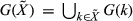
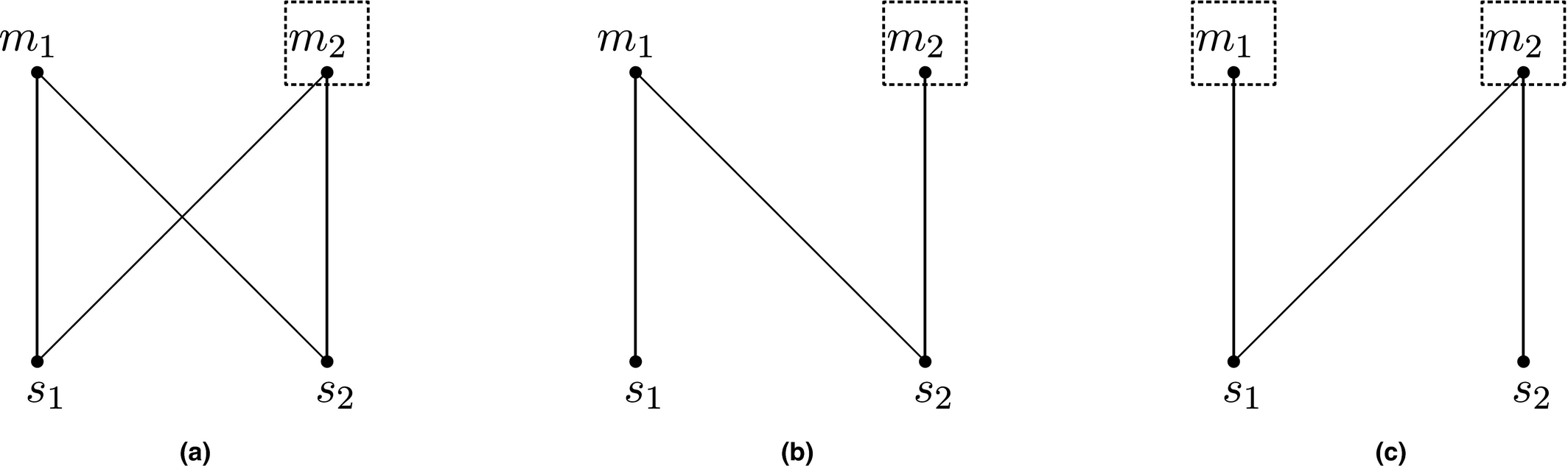
Because we represent the business relationship using a non‐directed bipartite graph, it is useful to introduce the following concepts. A firm that is linked with firm k in G = (S, M, L) is called a neighbor of k and the set of all neighbors of k is denoted by G(k) = {i ∈ S ∪ M|ki ∈ L or ik ∈ L}. Furthermore, we denote the neighbors of the set

\tilde{X} \subseteq X

G (\tilde{X}) = ⋃_{k \in \tilde{X}} G (k)

where X ∈ {S, M}. A subgraph

\tilde{G} = (\tilde{S}, \tilde{M}, \tilde{L})

of G is a graph such that

\tilde{S} \subseteq S

\tilde{M} \subseteq M

, and the restriction of L over

\tilde{S} \cup \tilde{M}

, denoted as

\tilde{L} {= L |}_{\tilde{S} \cup \tilde{M}}

. A path in a graph is a sequence of nodes such that from each of its nodes there is a link to the next node in the sequence. A bipartite graph is connected if there exists a path linking any two nodes of the graph. Although they are slightly different concepts, throughout the study, we use the terms “network” and “graph” interchangeably. We only consider supply networks whose business relationship graphs are connected. If the supply network's business relationship graph is disconnected, we can apply all of our results to each disconnected component of the network separately.

Preliminaries

We will analyze several simple supply chain networks with at most two suppliers and two manufacturers. The results about these simple networks can offer helpful insight for understanding larger and more general networks. Throughout the study, by uniqueness, we refer to the uniqueness in terms of equilibrium payoffs not equilibrium strategies.

We start with the cases in which there are at most three firms in the supply chain. In the simplest case, there is only one supplier and one manufacturer in the network and the firms engage in the well‐known alternating offer bargaining game of Rubinstein (1982). For this case, the unique equilibrium price is

\frac{δ}{1 + δ} v

, which implies that the equilibrium payoffs are

\frac{1}{1 + δ} v

for the manufacturer and

\frac{δ}{1 + δ} v

for the supplier.

When two homogenous suppliers are linked to one manufacturer with valuation v, the manufacturer can take advantage of the competition between two homogenous suppliers to press the price down to their reservation values, which are all zero. With price at zero, the manufacturer collects all the economic surplus of the trade and receives a payoff of v. In contrast, when one supplier is linked to two heterogenous manufacturers with valuations v ₁ and v ₂, the supplier cannot collect all the economic surplus of the trade, which implies that the advantage of the supplier on the short side is limited in the presence of valuation heterogeneity among the manufacturers on the long side. The advantage of the supplier on the short side of the network would push the price up, however, with heterogenous valuations, the price cannot be pushed all the way up to the valuation of the manufacturer who would eventually win the trade. This is because as the price reaches the lower valuation of the two manufacturers, v ₂, the manufacturer with valuation v ₂ would drop out of the competition and the manufacturer with valuation v ₁ would be the only buyer left in the market to win the trade. Given the assumption

\underset{̲}{v} \geq \frac{δ}{1 + δ} \bar{v}

or specifically

v_{2} \geq \frac{δ}{1 + δ} v_{1}

in this case (this assumption ensures that the two manufacturers are meaningful competitors), the supplier would prefer to accept the price v ₂ right away than bargaining with the manufacturer with valuation v ₁ further in the next period. In other words, with heterogenous valuations, the manufacturers are differentiated. This degree of differentiation would help the manufacturer with higher valuation to partially offset the pricing advantage of the supplier on the short side. With this protection from differentiation, the manufacturer with higher valuation can enjoy some surplus of the trade and prevent the supplier from collecting all the surplus.

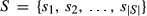
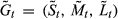
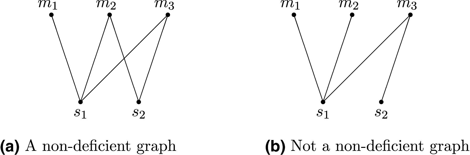
We now consider networks in which there are two suppliers, s ₁ and s ₂ and two manufacturers, m ₁ and m ₂ with valuations v ₁ > v ₂. There are three possible connected supply chain network structures, which are shown in Figure 1. Notice that in these networks, supply and demand are perfectly balanced because there are equal number of firms on both sides of the networks. The equilibrium outcomes of these networks are summarized in the next proposition.

Figure 1

All Possible Connected Supply Chain Networks with Two Suppliers and Two Manufacturers

Proposition 1

Consider a supply chain network with two suppliers, s ₁ and s ₂ and two manufacturers, m ₁ and m ₂, with valuations v ₁ and v ₂ where v ₁ > v ₂.

In the supply chain networks in Figure 1a and b, there exists a unique subgame perfect Nash equilibrium where all firms trade at price

\frac{δ}{1 + δ} v_{2}

;

In the supply chain network in Figure 1c, there exists a unique subgame perfect Nash equilibrium where supplier s ₁ trades with manufacturer m ₁ at price

\frac{δ}{1 + δ} v_{1}

and supplier s ₂ trades with manufacturer m ₂ at price

\frac{δ}{1 + δ} v_{2}

Proof 1

All proofs are provided in Appendix A. □

From the discussion above, we know that the valuation heterogeneity can allow the high valuation manufacturer to press down the price and collect some surplus in a supply chain with three firms. Proposition 1 indicates that whether the valuation heterogeneity can protect the high valuation manufacturer in a supply chain with four firms critically depends on whether the high valuation manufacturer is well connected (i.e., has more than one link) in the network or not. Specifically, in the supply chain networks in Figure 1a and b, the high valuation manufacturer, m ₁ is well connected because she is linked to both suppliers in the network. So, the high valuation manufacturer, m ₁ is able to trade at price

\frac{δ}{1 + δ} v_{2}

, which is lower than the price (

\frac{δ}{1 + δ} v_{1}

) she would pay if she bargains with a supplier independently. In contrast, in the supply chain network in Figure 1c, the high valuation manufacturer, m ₁ is not well connected because she is linked to only one supplier, s ₁. As a result, supplier s ₁ will strategically isolate manufacturer m ₁ to engage a Rubinstein bargaining game and trade with her at a higher price

\frac{δ}{1 + δ} v_{1}

Notice that when the manufacturers have homogenous valuation, network structure would not affect equilibrium prices at all because all three possible networks shown in Figure 1a–c are essentially equivalent, in price and payoff terms, to two independent linked pairs whose equilibrium would be determined according to the Rubinstein bargaining game (see Corominas‐Bosch 2004 for detailed discussions of the intuition of this result). Intuitively, since all suppliers and manufacturers are homogenous in this case, they are really indifferent about who to trade with. The sharp contrast between the equilibrium of two similar networks in Figure 1b and c allows us to see clearly why network structure plays an important role on influencing equilibrium prices and payoffs when manufacturers have heterogenous valuations. In the supply chain network in Figure 1c, we end up with two different prices in equilibrium. So, when manufacturers have heterogeneous valuations, suppliers’ preferences to trade with manufacturers with high valuations lead to more prices or price dispersion in a supply chain network because the exact price a supplier can get from a trade critically depends on the exact valuation of the manufacturer involved in the trade.

The results about the simple supply chain networks reveal the rich dynamics among three fundamental factors: the balance between supply and demand, valuation heterogeneity, and network structure on jointly determining equilibrium prices and payoffs in a supply chain network. When the manufacturers have heterogenous valuations, valuation heterogeneity can potentially act as a countering force to limit the pricing power of the suppliers in supply chains with less suppliers than manufacturers. In addition, valuation heterogeneity makes network structure, specifically how manufacturers with higher valuations are connected in a network, relevant in determining the equilibrium. Furthermore, we have also learned that not all links in a supply chain network are relevant because firms could strategically ignore some of them. Bargaining in a supply chain network will likely happen in smaller subnetworks where the three fundamental factors will determine the equilibrium for each of them. In the next section, we carry these results and insights into more general supply chain networks.

General Supply Chain Networks

We will examine general supply chain networks in this section. To study general supply chain networks, we first need to introduce a set of technical concepts from graph theory.

Definitions

Let G = (S, M, L) be the underlying bipartite graph of a supply chain network (G, v).

Definition 1

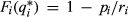
A bipartite graph G is “non‐deficient” if and only if

| G (S^{'}) | \geq | S^{'} |

for any subset S ^′ ⊆ S of size

| S^{'} | \leq | M |

| G (M^{'}) | \geq | M^{'} |

for any subset M ^′ ⊆ M of size

| M^{'} | \leq | S |

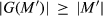
Non‐deficiency requires that every subset of firms on the long side of a network has enough neighbors to trade. Figure 2 provides a network that satisfies non‐deficiency requirement in (a) and a network that does not in (b). Notice that manufacturers are on the long sides of both networks. The network in (a) is non‐deficient because in any subsets (i.e., {m ₁}, {m ₂}, {m ₃}, {m ₁, m ₂}, {m ₁, m ₃}, and {m ₂, m ₃}) of the long side of the network M, the manufacturers with no more than two manufacturers (|S| = 2) are all linked to at least the same number of suppliers so that all manufacturers are guaranteed to trade. The network in (b) does not satisfy the non‐deficiency requirement since the subset {m ₁, m ₂} is collectively linked to only one supplier {s ₁} which implies either m ₁ or m ₂ will not be able to trade. Notice that non‐deficiency is defined for the long side of a bipartite graph and does not imply that both sides of the graph have to satisfy the condition.

Figure 2

Non‐Deficiency of Graphs

Because the valuations of the manufacturers are different in our setting, the following definitions of manufacturer types play a crucial role in our results.

Definition 2

Let G be a non‐deficient bipartite graph that contains a perfect matching. A manufacturer

m_{i} \in M

is a “moderate manufacturer” if

| G (m_{i}) | = 1

or,

| G (m_{i}) | > 1

and

v_{i} = min {v_{j} | m_{j} \in C_{G} (m_{i})}

where

C_{G} (m_{i}) = ⋂_{s \in G (m_{i})} G (s)

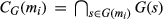
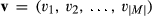
Moderate manufacturers are defined in a bipartite graph that contains a perfect matching or has equal number of firms on both sides. The definition says that a manufacturer is moderate if (i) she is connected to only one supplier or (ii) she has the lowest valuation among all her competing manufacturers. The set of moderate manufacturers in a supply chain network is always non‐empty since, in any bipartite graph with a perfect matching, the manufacturer with the lowest valuation is by definition a moderate manufacturer. Moderate manufacturers in a supply chain network are basically disadvantageous manufacturers in terms of either connection or valuation or both. Figure 3 identifies the moderate manufacturers for the supply chain networks in Proposition 1. Notice that the networks in Figure 3a and b have only one moderate manufacturer m ₂ who has the lowest valuation as compared to her competitor m ₁ for s ₁ in (a) and has only one link in (b), whereas the network in Figure 3c has two moderate manufacturers m ₁ who has only one link, and m ₂ who has the lowest valuation as compared to her competitor m ₁ for s ₁. As we will see in the next section, this difference will play a crucial role in determining the equilibrium strategies of the firms.

Figure 3

Moderate Manufacturers

Although moderate manufacturers are disadvantageous to their rivals due to their limited connections and/or low valuations, they can still trade at the end of the bargaining process because of the balanced supply and demand in a network with perfect matching. However, in networks with more manufacturers than suppliers or more demand than supply, there is no perfect matching anymore. In such networks, some manufacturers with low valuations, contrary to moderate manufacturers, will not be able to trade due to the scarcity of suppliers. We need to differentiate such manufacturers from moderate manufacturers.

Definition 3

Let G be a non‐deficient bipartite graph with manufacturer side is longer; that is, |M| > |S|. A manufacturer

m_{i} \in M

is a “soft manufacturer” if v _i ≤ v _s where v _s is the (|S| + 1)th highest valuation in G. Furthermore, the “critical soft manufacturer” of G is the manufacturer with the valuation v _s, which is denoted by m _s.

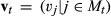
The main difference between soft and moderate manufacturers is that moderate manufacturers, although disadvantageous, are able to trade whereas soft manufacturers are not. Figure 4 shows a network with two suppliers and five manufacturers. Suppose that the manufacturer valuations are ranked as v ₁ > ⋯ > v ₅. Then, the manufacturers m ₃, m ₄, and m ₅ are all soft manufacturers since they have valuations less than v _s, which is equal to v ₃ because |S| + 1 = 3 in this case. Furthermore, m ₃ is the critical soft buyer since he has (exactly) the third (|S| + 1) highest valuation among all the manufacturers in the network. In supply chains where there are more suppliers than manufacturers, none of the manufacturers are moderate or soft since all manufacturers are on the short side of the network. We are now ready to define three types of supply chain networks.

Figure 4

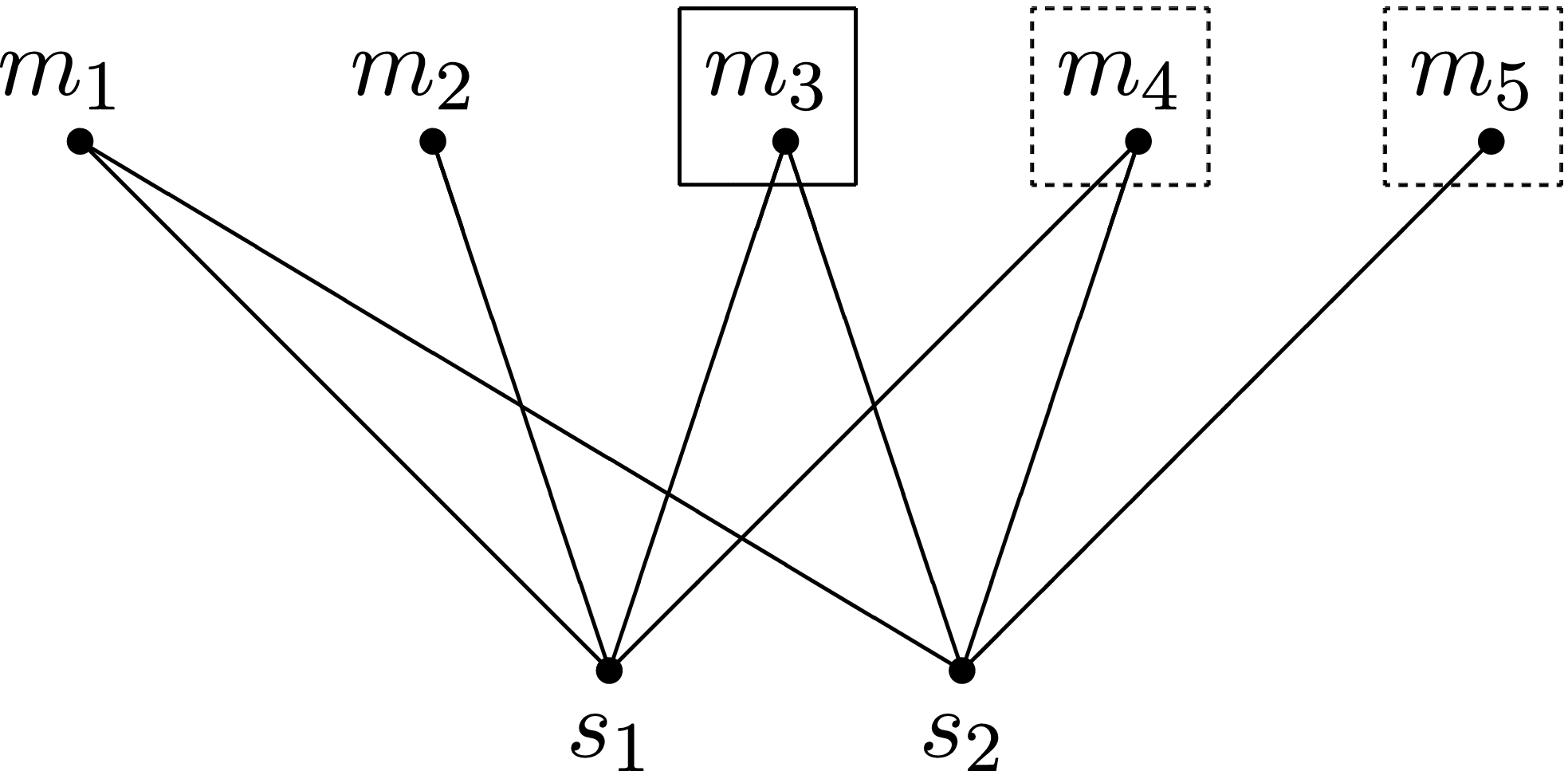
Soft Manufacturers (dashed boxes) and the Critical Soft Manufacturer (solid box)

Definition 4

A supply chain network (G, v) is type

(G, v)^S if |S| > |M| and G is non‐deficient;

{(G, v)}_{k}^{E}

if |S| = |M| and G is non‐deficient with the moderate manufacturer m _k;

{(G, v)}_{s}^{M}

if |M| > |S| and G is non‐deficient with the critical soft manufacturer m _s.

In addition, we say that the underlying graph of a supply chain network is G ^S,

G_{k}^{E}

, or

G_{s}^{M}

type if it belongs to a network that is of type (G, v)^S,

{(G, v)}_{k}^{E}

, and

{(G, v)}_{s}^{M}

, respectively. It is easy to see that not every graph is one of these types. For example, Figure 2b demonstrates a network that is not one of these three types. To see why, notice that in Figure 2b the number of manufacturers is higher than the number of suppliers, the network can only be

{(G, v)}_{s}^{M}

type and we only need to check the condition (iii) of the definition. As we have already identified that this network does not satisfy the non‐deficiency condition ({m ₁, m ₂} are linked with {s ₁} only), this graph is not a

G_{s}^{M}

type either.

Decomposition of General Supply Chain Networks

One insight we learned from the analysis of small supply chain networks was that not all links in a supply chain network are relevant (because firms could strategically ignore some of the links) and bargaining in a supply chain network will happen in smaller subnetworks in equilibrium. This insight implies that we can significantly simplify the analysis for general and more complex supply chain networks by focusing on these smaller subnetworks. We now provide a network decomposition algorithm, which allows us to identify the subnetworks of a general supply chain network where bargaining will take place in equilibrium. The decomposition we will describe below has close connections with the canonical structure theorem of Gallai and Edmonds, which shows a unique decomposition of any graph into three set of subgraphs.²

The decomposition algorithm we propose builds on the earlier algorithms (e.g., the algorithm for networks with homogenous buyers by Corominas‐Bosch 2004), and provides a finer decomposition of the network since it takes the manufacturer valuations into account. We provide the summary of algorithm here and defer the detailed description of it to Appendix B. Figure 5 provides an example to illustrate the steps of the algorithm. The algorithm is consist of three main parts. First, the algorithm checks all possible subgraphs for the existence of G ^M type subgraphs lexicographically in an ascending order of size starting with the manufacturer m ₁ and separates them from the graph iteratively until no more G ^M type subgraphs can be found. Figure 5b shows the subgraph

G_{4}^{M}

identified and the remaining graph after removing

G_{4}^{M}

in the example. Second, once the algorithm removes the G ^M type of subgraphs, it repeats the same process on the remaining graph in order to identify and remove the G ^S type of subgraphs. Figure 5c shows the two subgraphs,

G_{4}^{M}

and G ^S the algorithm identifies so far, and the remaining graph after the the subgraphs are removed in the example. Third, for the G ^E type of subnetwork structures, the algorithm uses the information about the manufacturer valuations to decompose the set of G ^E type subgraphs further into smaller subgraphs as follows. First, the algorithm finds all moderate manufacturers and remove all links between the following nodes: (i) suppliers who are connected to the moderate manufacturer with the highest valuation and (ii) manufacturers who have valuations lower than the highest valued moderate manufacturer. Then, the algorithm removes the links between suppliers who are connected to the moderate manufacturer with the second highest valuation and manufacturers who have valuations lower than the second highest valued moderate manufacturer. The algorithm continues removing links in this fashion until there are no moderate manufacturers. At the end of this process, we may end up having more than one subgraph. The algorithm labels these subgraphs as

G_{k}^{E}

where k is the subindex of the manufacturer with the lowest valuation in that subgraph. Two G ^E type subgraphs,

G_{5}^{E}

and

G_{6}^{E}

are identified in the example, and the final decomposition of the example network is shown in Figure 5d.

Figure 5

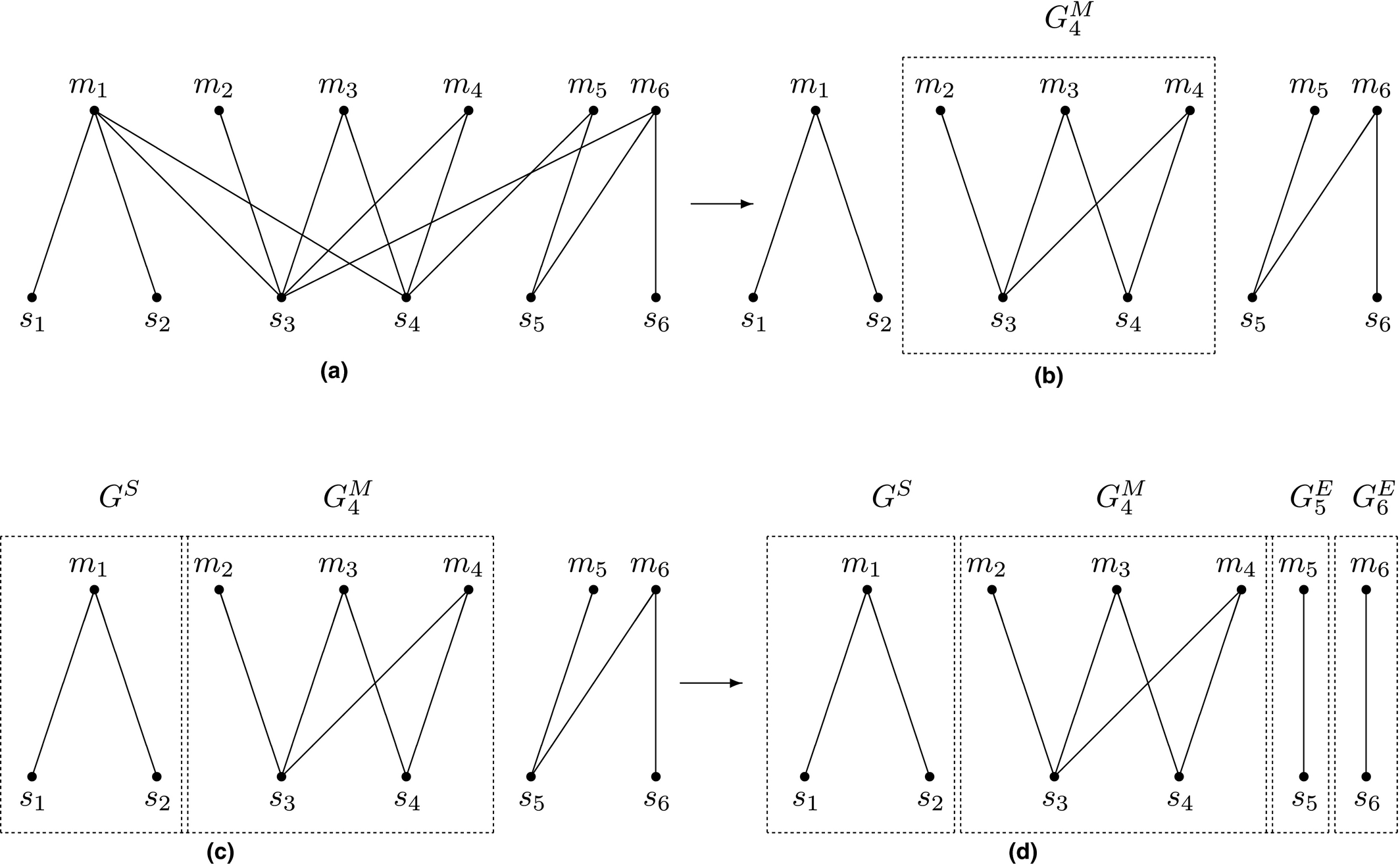
The Decomposition of a General Supply Chain Network with Heterogeneous Manufacturer Valuations into Subnetworks

Notice that at the end of the algorithm the manufacturer with the lowest valuation in the subnetwork

{(G, v)}_{k}^{E}

has to be the only moderate manufacturer in that subnetwork. Thus, the number of moderate manufacturers determines the number of subnetworks that are of type

{(G, v)}_{k}^{E}

. Intuitively, for

{(G, v)}_{k}^{E}

type of subnetworks, the algorithm removes all the redundant links from the suppliers’ perspectives since being connected to a moderate manufacturer limits the minimum earning of a supplier. Suppliers that are connected to moderate manufacturers will never consider trading with the manufacturers with lower valuations, which implies the underlying graph structure of the supply chain can be decomposed further into smaller subgraphs.

Equilibrium Prices in General Supply Chain Networks

We are now ready to show the subgame perfect Nash equilibrium for a general supply chain network which can be decomposed into three types of subnetworks, using the decomposition algorithm presented in section 5.2. The following proposition specifies the subgame perfect Nash equilibrium for each of the three types of subnetwork in a general supply chain network.

Proposition 2

Let (G, v) be a supply chain network. Then, there exists a unique (in terms of payoffs) subgame perfect Nash equilibrium such that a supplier trades with a manufacturer m _i with valuation v _i in a subnetwork

(\tilde{G}, \tilde{v})

at price

{\tilde{p}}_{i} = \{\begin{matrix} 0, & i f (\tilde{G}, \tilde{v}) i s o f t y p e {(G, v)}^{S}; \\ \frac{δ}{1 + δ} {\tilde{v}}_{k}, & i f (\tilde{G}, \tilde{v}) i s o f t y p e {(G, v)}_{k}^{E}; \\ {\tilde{v}}_{s}, & i f (\tilde{G}, \tilde{v}) i s o f t y p e {(G, v)}_{s}^{M} . \end{matrix}

where

{\tilde{v}}_{k}

and

{\tilde{v}}_{s}

are the moderate and critical soft manufacturers in the subnetwork

(\tilde{G}, \tilde{v})

when

(\tilde{G}, \tilde{v})

is of type

{(G, v)}_{k}^{E}

and

{(G, v)}_{s}^{M}

, respectively. The equilibrium payoff for the supplier is

{\tilde{p}}_{i}

, and the equilibrium payoff for the manufacturer m _i is

v_{i} - {\tilde{p}}_{i}

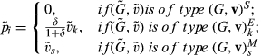
The proof of Proposition 2 is by induction on the number of firms on both sides of a supply chain network. First, the small supply chain results in section 4 are special cases of Proposition 2. Let us check Proposition 2 on the networks with at most two manufacturers and two suppliers. The network with one supplier linked with one manufacturer is a

{(G, v)}_{k}^{E}

type with

{\tilde{v}}_{k} = v

, so the equilibrium price is

\frac{δ}{1 + δ} v

. The network with two suppliers linked with one manufacturer is a (G, v)^S type, so the equilibrium price is 0. The network with one supplier linked with two manufacturers are

{(G, v)}_{s}^{M}

type with

{\tilde{v}}_{s} = v_{2}

, so the equilibrium price is v ₂. Now consider the networks in Proposition 1. The networks in part (i) are

{(G, v)}_{k}^{E}

type with

{\tilde{v}}_{k} = v_{2}

, so the equilibrium price is

\frac{δ}{1 + δ} v_{2}

. The network in part (ii) can be decomposed into two independent

{(G, v)}_{k}^{E}

type subnetworks with

{\tilde{v}}_{k} = v_{1}

and

{\tilde{v}}_{k} = v_{2}

, respectively, so the equilibrium prices are

\frac{δ}{1 + δ} v_{1}

and

\frac{δ}{1 + δ} v_{2}

, respectively. Therefore, Proposition 2 is true for the supply chain networks that have at most two suppliers and two manufacturers. Then, we assume that Proposition 2 is true for supply chain networks that have at most n − 1 suppliers and n − 1 manufacturers, and show that the proposition also holds for supply chain networks that have at most n suppliers and n supply chain networks.

In a type (G, v)^S network, we have more supply (suppliers) than demand (manufacturers). The supply and demand balance in this case favors the manufacturers and presses the prices down to the suppliers’ reservation values, which are homogenous zero. Thus, the suppliers capture zero surplus from the trades while the manufacturers extract all the surplus. However, in a type

{(G, v)}_{s}^{M}

network, we have more demand (manufacturers) than supply (suppliers). The supply and demand balance in this case favors the suppliers and pushes the prices up to the valuation of the critical soft manufacturer, v _s. As a result, in a type

{(G, v)}_{s}^{M}

network, valuation heterogeneity among the manufacturers limits the un‐favoring supply and demand balance situation. With the protection of valuation heterogeneity, the manufacturers are able to retain some surplus in a disadvantageous market for them. Finally, in a type

{(G, v)}_{k}^{E}

network, there are equal numbers of suppliers and manufacturers, that is, supply and demand are perfectly balanced. So, all manufacturers will be able to trade. The equilibrium prices of trades are determined according to the moderate manufacturer's valuation v _k, which is the lowest among valuations of all manufacturers in that subnetwork. Hence, valuation heterogeneity protects the manufacturers and allows them to collect some surplus in a type

{(G, v)}_{k}^{E}

network too. Note that in

{(G, v)}_{s}^{M}

and

{(G, v)}_{k}^{E}

networks, the equilibrium prices depend on the exact valuations of the critical soft manufacturer and the moderate manufacturer, respectively. Therefore, there could be more prices or price dispersion than the cases where manufacturers have homogenous valuation.

In Figure 6, we apply Proposition 2 to the network that is considered in Figure 5. By applying the decomposition algorithm on the network, we have identified subnetworks with types G ^S,

G_{4}^{M}

G_{5}^{E}

, and

G_{6}^{E}

. Then, according to Proposition 2, we can determine the equilibrium prices in each of these subnetwork: The price in G ^S is 0, in

G_{4}^{M}

is v ₄, in

G_{5}^{E}

\frac{δ}{1 + δ} v_{5}

and in

G_{6}^{E}

\frac{δ}{1 + δ} v_{6}

Figure 6

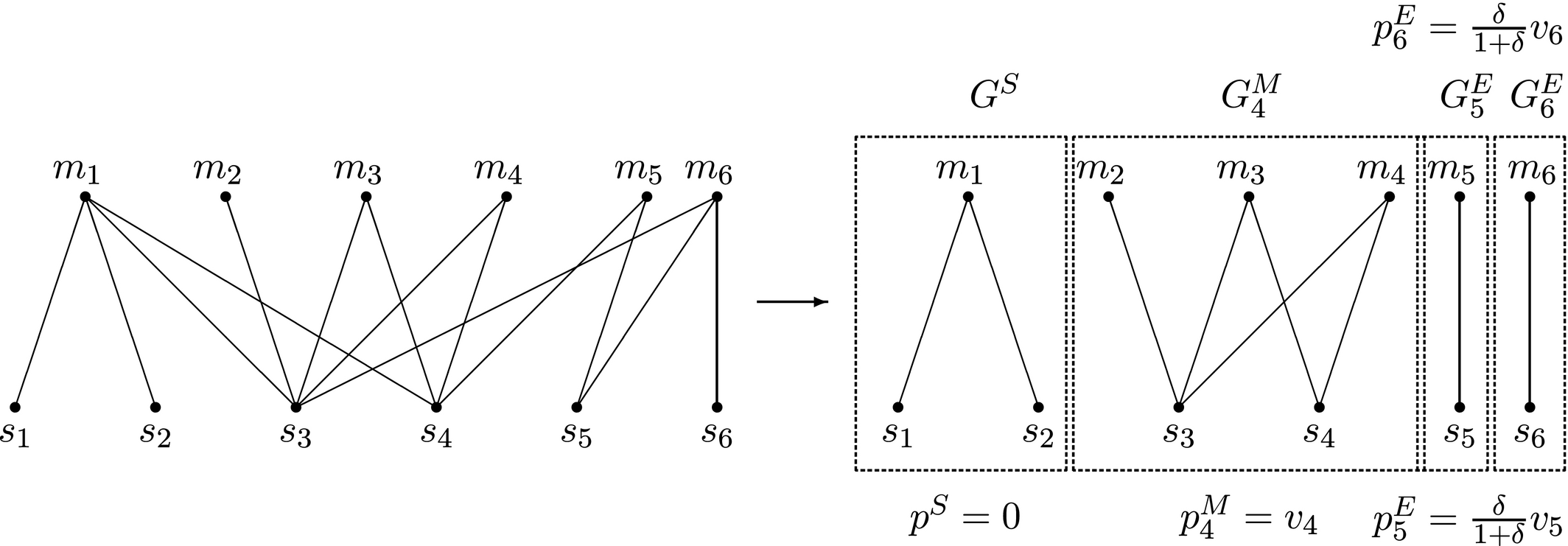
The Equilibrium for a Complex Supply Chain Structure

Efficient Supply Chain Networks

In this section, we investigate the efficiency of supply chain networks which is a unique issue when manufacturers’ values are different. Network structure not only impacts the equilibrium prices but also determines the set of feasible trading patterns or allocation of goods. It is possible that manufacturers who have the highest valuations are not necessarily able to trade in equilibrium due to the restrictions of network structure. This inefficiency will lead to a loss of economic surplus. In order to examine the welfare properties, we define a supply chain network (G, v) as “efficient” if only the manufacturers with the highest valuations are able to trade in the equilibrium. Note that with homogeneous manufacturer valuations, as in Corominas‐Bosch (2004), this is not a concern and all supply chain networks are efficient.

Proposition 3

A supply chain network (G, v) is efficient if and only if after decomposition, either there are no

G_{s}^{M}

subnetworks or all soft manufacturers in

G_{s}^{M}

subnetworks have valuations less than or equal to the (|S| + 1)th highest manufacturer valuation.

Recall that a soft manufacturer is defined for type

G_{s}^{M}

network in which there are more manufacturers than suppliers. If a supply chain network can be decomposed into only type G ^S and type

G_{k}^{E}

subnetworks, there are no soft manufacturers. In type G ^S or type

G_{k}^{E}

subnetworks, there is enough supply (i.e., suppliers) to guarantee all manufacturers in the networks to be able to trade in equilibrium. So, these two types of subnetworks always provide efficient allocations. Therefore, the original supply chain network is efficient. However, if the decomposition of a supply chain network includes type

G_{s}^{M}

subnetworks, there is a supply shortage (i.e., less suppliers than manufacturers) in these subnetworks so that soft manufacturers who are not well connected (i.e., with only one link) will not be not able to trade. Then, allocation efficiency becomes a concern. To ensure that the manufacturers with the highest valuations in a type

G_{s}^{M}

subnetwork are able to trade, they should be well connected with more than one link, that is, not be the soft manufacturers in the type

G_{s}^{M}

subnetworks.

Figure 7 provides examples of inefficient and efficient supply chain networks. The network on the left is inefficient since m ₂ cannot trade in the equilibrium. If we apply Proposition 3 to this example, the supply chain network is decomposed into a

G_{2}^{M}

subnetwork and a

G_{3}^{E}

subnetwork. The soft manufacturer in the

G_{2}^{M}

subnetwork is manufacturer m ₂ whose valuation v ₂ is higher than the third (|S| + 1 = 3) highest manufacturer valuation, which is v ₃. In this example, the inefficiency is caused by the fact that manufacturer m ₂ is not well connected (due to only one link) and has to compete with manufacturer m ₁ to trade with supplier s ₁, while manufacturer m ₃ with lower valuation is well connected and can be guaranteed to trade. If we switch the positions of m ₂ and m ₃, we have the network on the right which is an efficient network because in the equilibrium, m ₁ and m ₂ who have the highest valuations in the network will trade while m ₃ will not. If we apply the Proposition 3 to this example, the supply chain network is decomposed into a

G_{3}^{M}

subnetwork and a

G_{2}^{E}

subnetwork. The soft manufacturer in the

G_{3}^{M}

subnetwork is manufacturer m ₃, whose valuation v ₃ is indeed the third highest manufacturer valuation.

Figure 7

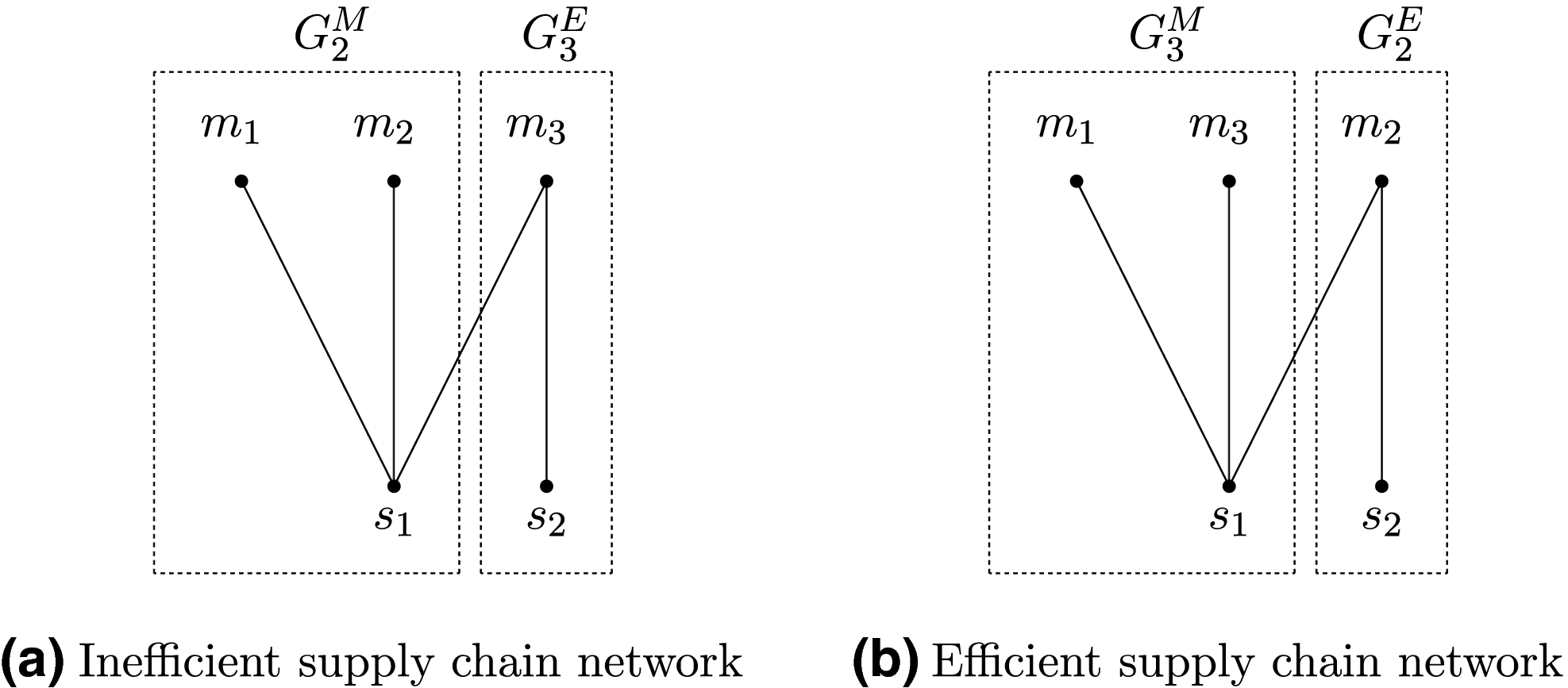
Inefficient vs. Efficient Supply Chain Networks

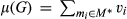
Next, we consider the impact of adding a new link on the efficiency of a supply chain network. Because efficiency is about the total surplus, we use the total surplus in equilibrium as a measure of the degree of efficiency of a supply chain network. Let

μ (G) = \sum_{m_{i} \in M^{*}} v_{i}

be the total surplus created in the equilibrium for the supply chain network (G, v) where M* represents the set of manufacturers that trade in the equilibrium.

Definition 5

A supply chain network (G, v) becomes more efficient after adding a link ij ∉ L between manufacturer

m_{i} \in M

and supplier

s_{j} \in S

in G if and only if μ(G + ij) > μ(G), where G + ij is the graph created by adding the link ij to G.

Proposition 4

Consider a supply chain network (G, v). Let G + ij be the graph created by adding a link ij ∉ L between manufacturer

m_{i} \in M

and supplier

s_{j} \in S

in G.

Adding the link ij does not improve efficiency, that is μ(G + ij) = μ(G), if

m _i and s _j belong to the same subnetwork;

both m _i and s _j belongs to a subnetwork of type G ^S or

G_{k}^{E}

;

s _j belongs to a subnetwork of type

G_{s}^{M}

Adding the link ij improves efficiency, that is μ(G + ij) > μ(G), if

m _i belongs to a subnetwork of type

G_{s}^{M}

with only one soft manufacturer, s _j belongs to a subnetwork of type

G_{k}^{E}

, and v _s > v _k;

m _i belongs to G _i, which is of type

G_{s}^{M}

with only one soft manufacturer, s _j belongs to G _j, which is of type G ^S, and

| S_{i} + S_{j} | = | M_{i} + M_{j} |

m _i belongs to a subnetwork of type

G_{s}^{M}

with multiple soft manufacturers, s _j belongs to a subnetwork of type

G_{k}^{E}

, and v _i > v _k;

To improve the efficiency of the supply chain network, adding a new link must lead to one or both of the following two changes in the network: (i) the total number of trades in the network increases so that more manufacturers will get a good; (ii) the trade matching between suppliers and manufacturers changes in such a way that the manufacturers with higher valuations get the goods. First, Part (i) of the above proposition identifies what types of link do not lead to any one of the above two changes when added, therefore not improving the efficiency of the supply chain network. Part (ia) is straightforward and indicates that adding a link that connects a manufacturer and a supplier within the same subnetwork will not change the allocation of goods and the efficiency of the network. Parts (ib) identifies cases where all manufacturers in a subnetwork have been able to trade already before adding the new link. Hence, adding the new link would not change the efficiency at all. This happens when both m _i and s _j belongs to a subnetwork of type G ^S (all manufacturers are able to trade because there are more suppliers than manufacturers) or when both m _i and s _j belongs to a subnetwork of type

G_{k}^{E}

(all manufacturers are able to trade because there are equal number of suppliers and manufacturers). In part (ic), if a supplier belongs to a

G_{s}^{M}

subnetwork with more manufacturers than suppliers, then the supplier already has an advantageous bargaining position in the subnetwork and will be able to trade whether there is a new link or not. Adding a new link connecting this supplier with a manufacturer is redundant and will be ignored by the supplier. Therefore, it will not improve the efficiency of the network.

Part (ii) of the Proposition 4 identifies cases where adding a link will improve the efficiency of the supply chain network. In particular, the proposition considers a new link that connects a manufacturer in a

G_{s}^{M}

subnetwork, which has more manufacturers than suppliers, to a supplier in another subnetwork. Because there are more manufacturers than suppliers in a

G_{s}^{M}

subnetwork, some manufacturers will not be able to trade, which provides opportunity for improvement. Part (iia) says that adding a link that connects a manufacturer in a

G_{s}^{M}

subnetwork with only one soft manufacturer to a supplier in a

G_{k}^{E}

subnetwork would improve the efficiency of the supply chain network. While the total number of trades stays the same in such a case, the additional link improves the efficiency by allowing better allocation of the goods: that is, the manufacturer m _s who is the critical soft manufacturer of subnetwork

G_{s}^{M}

will receive a good instead of m _k, who is the moderate manufacturer of subnetwork

G_{k}^{E}

, because m _s has higher valuation than m _k (i.e., v _s > v _k). Part (iib) suggests that adding a link that connects a manufacturer in a

G_{s}^{M}

subnetwork to a supplier in a G ^S subnetwork, which has more suppliers than manufacturers would improve the efficiency of the supply chain network if the two subnetworks merge into a G ^E type subnetwork (i.e.,

| S_{i} + S_{j} | = | M_{i} + M_{j} |

). Such a merge would lead to better match between supply and demand in the supply chain network which improves efficiency. Part (iic) of the proposition demonstrates the case where after adding a link between manufacturer m _i and supply s _j, the manufacturer m _i would leave her original subnetwork and join the supplier s _j's subnetwork that has lower valuation manufacturers. As a result, although the number of trades does not change in the supply chain network, the manufacturer m _i benefits from the additional link since it allows her to compete with lower valuation manufacturers. So, adding the link improves the efficiency since m _i will replaces supplier s _j's subnetwork's original moderate manufacturer m _k, who has lower valuation than m _i (v _i > v _k), to trade in the new subnetwork.

Discussions, Extensions, and Limitations

In this section, we compare our results with the most closely related models in the literature, and discuss some potential extensions and limitations of our model.

Cooperative Bargaining

We use a non‐cooperative bargaining setup where the firms negotiate via a generalized version of Rubinstein bargaining game. Another approach would be to consider a cooperative setup with Nash bargaining framework. In the Nash bargaining framework, the focus is not on the strategic interactions between firms but more on the “reasonable” outcomes that satisfy certain plausible conditions such as Pareto optimality and Independence of Irrelevant Alternatives.

Kleinberg and Tardos (2008) provides an analysis of Nash bargaining solution in the network setting. To illustrates the differences between our results and Nash bargaining solution, consider the network in Figure 1c under the assumption that δ = 1 for all firms and v ₁ = v ₂ = 1. To calculate the Nash bargaining solution, we need to determine the outside option for each firm. In the example, the outside options of m ₁ and s ₂ are zero since they have only one link. Let α ₂ be the outside option of manufacturer m ₂ when she is negotiating with s ₂ and let β ₁ be the outside option of supplier s ₁ when he is negotiating with m ₁. Recall that the Nash bargaining solution prescribes that the parties that negotiate each get their outside option plus the half of the surplus. Then, the outcome for manufacturer m ₂ is

α_{2} + \frac{1}{2} (1 - α_{2})

from his negotiation with s ₂. In other words, if s ₁ wants to trade with m ₂, he needs to offer at least

α_{2} + \frac{1}{2} (1 - α_{2})

and receive

1 - (α_{2} + \frac{1}{2} (1 - α_{2}))

for himself. From the latter expression, we can conclude that

β_{1} = \frac{1}{2} (1 - α_{2})

. Similarly, the outcome for supplier s ₁ is

β_{1} + \frac{1}{2} (1 - β_{1})

from his negotiation with m ₁. Then,

α_{2} = \frac{1}{2} (1 - β_{1}) = \frac{1}{2} (1 - \frac{1}{2} (1 - α_{2}))

, which implies that α ₂ = 1/3 and β ₁ = 1/3. Thus, the unique outcome that supports the Nash bargaining solution in this setting is where m ₁ trades with s ₁ at the price p ₁ = 2/3 and m ₂ trades with s ₂ at the price p ₂ = 1/3. Our model predicts that the outcome involves the same trade pairs with prices p ₁ = p ₂ = 1/2.

Notice that in the Nash bargaining solution, the bargaining outcome has to consider the outcome where the firms s ₁ and m ₂ agree on a price. Neither of the firms has an option to ignore such an outcome in their negotiations. In our setting, s ₁ has incentive to ignore the potential negotiation outcome with m ₂, which works as a commitment device to his negotiation with m ₁. Therefore, we choose to use the Rubinstein bargaining framework in our model because it better reflects the reality of negotiations in supply chain network where firms often strategically ignore some of their links that do not generate value to their current negotiations.

Other Non‐Cooperative Exchange Networks

In this section, we compare our results with two other closely related papers in the literature: Kranton and Minehart (2001) and Manea (2011). Kranton and Minehart (2001) uses an auction model to determine market prices in a setting with valuation heterogeneity among buyers (i.e., manufacturers in our setting). They prove that it is an equilibrium for each buyer to remain in the bidding in each of its linked sellers’ auctions up to its valuation of a good. Thus, in Kranton and Minehart (2001) setup, buyers pay the lowest “Walrasian” price for a clearable set of sellers, which is defined as the subset of sellers for whom “demand equals supply” (i.e., G ^E type of subgraphs in our model terms). In other words, for any clearable set of sellers, there is a continuum of prices such that demand equals supply and the auction equilibrium picks out the lowest price. In our bargaining model, the equilibrium prices are not necessarily the lowest price that equals demand and supply. They are determined by the relative bargaining powers of firms.

Manea (2011) considers a network where each pair of players connected by a link can jointly produce a unit surplus. The network generates the following infinite horizon discrete time bargaining game. Each period a link is selected according to some probability distribution, and one of the two matched players is randomly chosen to make an offer to the other player specifying a division of the unit surplus between themselves. If the offer is accepted, the two players exit the game with the shares agreed on. Unlike our model, in Manea (2011), the two players who reached agreement are replaced in the next period by two new players at the same positions in the network. If the offer is rejected, the two players remain in the game for the next period. All players have a common discount factor δ. The following concepts are helpful in characterizing the limit equilibrium payoffs (i.e., when δ → 1). A non‐empty set of players is mutually estranged if it is G‐independent (i.e., they are not connected in G). The set of partners for a mutually estranged set M _i is defined as L _i (i.e., S _i = G(M _i)) and the shortage ratio of M _i is defined as the ratio of the number of partners to estranged players (i.e.,

r_{i} = | S_{i} | / | M_{i} |

). Manea (2011) shows that for high values δ, M _i cannot have more “collective bargaining power” than its partner set S _i.

As an illustration, consider the network with three manufacturers and two suppliers in Figure 8. In Manea (2011), the outcome is determined by the shortage ratio as follows. The relevant outcomes are r ₁ = 1/2, M ₁ = {m ₁, m ₂}, S ₁ = {s ₁} and r ₂ = 1, M ₂ = {m ₃}, S ₂ = {s ₂}. By Manea (2011) results, the limit equilibrium payoffs are given by r ₁/(1 + r ₁) = 1/3 for m ₁ and m ₂, 1/(1 + r ₁) = 2/3 for s ₁, and r ₂/(1 + r ₂) = 1/(1 + r ₂) = 1/2 for m ₃ and s ₂. In order to compare with our results, suppose in our model that v _i = 1 for all

m_{i} \in M

and δ = 1. Then, by Proposition 2, the equilibrium outcomes are 0 for m ₁ and m ₂, 1 for s ₁, and 1/2 for m ₃ and s ₂.

Figure 8

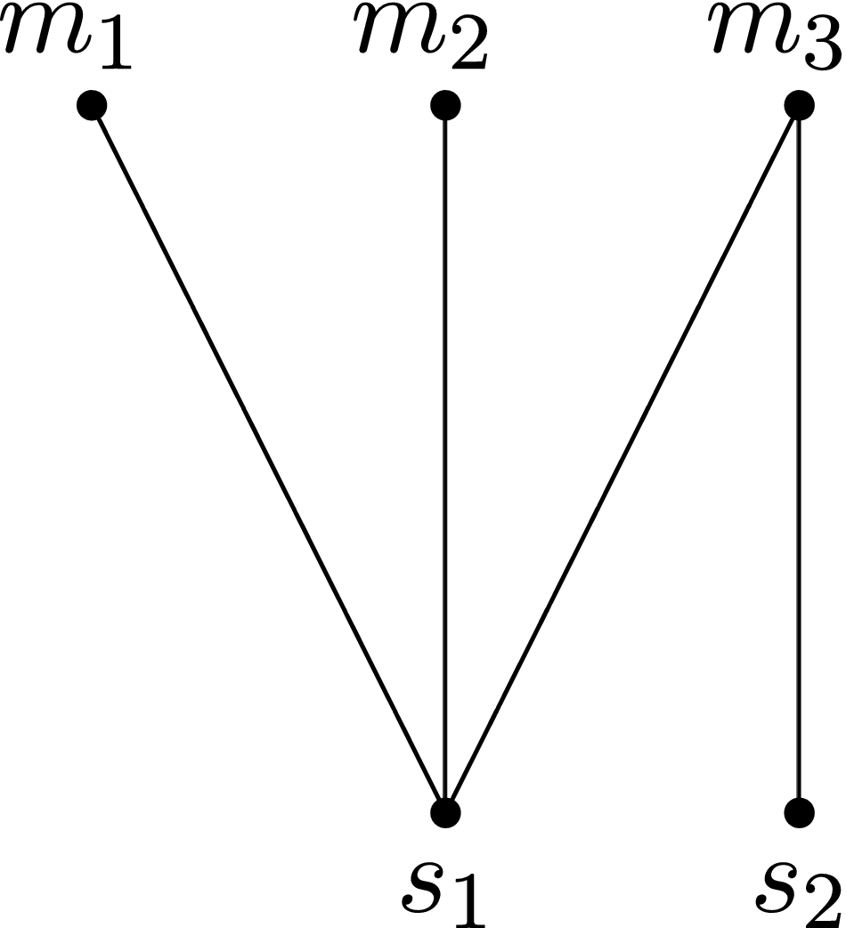
A Network that Produces Different Outcomes in Our Model and in Manea (2011)

This example shows that when one side is shorter, the competition is more intense in our setting than the one in Manea (2011) model. To examine this discrepancy, consider a scenario in which players m ₁ and s ₁ in Figure 8 are matched as in Manea (2011) model and reach an agreement with each other in the first period. Then, suppose that, m ₁ and s ₁ are removed from the network without replacement. In this case, m ₂ is left isolated and his continuation payoff is 0. By contrast, in the stationary economy described in Manea (2011), a new trader enters the market at the node s ₁ in the second period, and m ₂ may get a chance to bargain with this new trader. In equilibrium, m ₂ capitalizes on the perpetual rebirth of bargaining partners at node s ₁ to secure a limit payoff of 1/3. We can obtain our results in terms of shortage ratios by adjusting the Manea (2011)'s original theorem to include the effect of supply and demand mismatch, which is not a strong concern in Manea (2011) due to the replacement of players assumption. In particular, the adjusted outcome uses the original result of Manea (2011) only when supply and demand are balanced (i.e., r _i = 1). For the cases where one side of the market is shorter (i.e., r _i ≠ 1), the outcome uses our result under the assumptions that v _i = 1 for all

m_{i} \in M

and δ = 1. Notice that if we apply this adjusted outcome to the network in Figure 8, we have r ₁ = 1/2 < 1 and therefore in the limit equilibrium, m ₁ and m ₂ receive the payoff 0, whereas s ₁ receives 1. Since r ₂ = 1, both m ₃ and s ₂ receive the payoff 1/2. This is the same equilibrium outcome for our model.

Efficiency vs. Competitiveness

We have discussed the efficiency of supply chain networks that ensures the manufacturers with the highest valuations to be able to trade in equilibrium. Now, we consider the relationship between efficiency and competitiveness of a supply chain network. In a competitive supply chain network, the equilibrium price should be solely determined by the aggregate demand‐supply balance, and any other factors, such as network structure, should not restrict the equilibrium price or competition. Thus, in a competitive supply chain network, all trades should happen at a common price in our setting. To formally define the competitive supply chain network in our setting, we use a generalized version of Corominas‐Bosch (2004) definition.

Definition 6

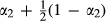
A supply chain network (G, v) is competitive, if

if |M| < |S|, then the equilibrium price is zero for all trades;

if |M| > |S|, then the equilibrium price is equal to the (|S| + 1)th highest manufacturer valuation for all trades;

if |M| = |S|, then the equilibrium price is equal to

\frac{δ}{1 + δ} \underset{̲}{v}

for all trades.

Not every network structure allows a supply chain network to be competitive. For example, consider the supply chain network in Figure 9 where three manufacturers and two suppliers. Because there are more manufacturers than suppliers, to be competitive, all trades in this supply chain network must happen at the price of v ₃ according to the definition. The network on the left in Figure 9 is a competitive enough to generate such a price for all trades, whereas the one on the right is not competitive enough to make it happen. In the latter case, notice that the network can be decomposed into a

G_{3}^{M}

subnetwork and a

G_{2}^{E}

subnetwork. We know immediately there will be two different prices in the equilibrium. While manufacturer m ₁ will trade with supplier s ₁ at price v ₃ in the

G_{3}^{M}

subnetwork, manufacturer m ₂ will bargain with the supplier s ₂ in the

G_{2}^{E}

subnetwork independently and will pay s ₂ only

\frac{δ}{1 + δ} v_{2}

, which is less than the competitive price v ₃. Next, we characterize the relationship between competitiveness and efficiency in supply chain networks.

Figure 9

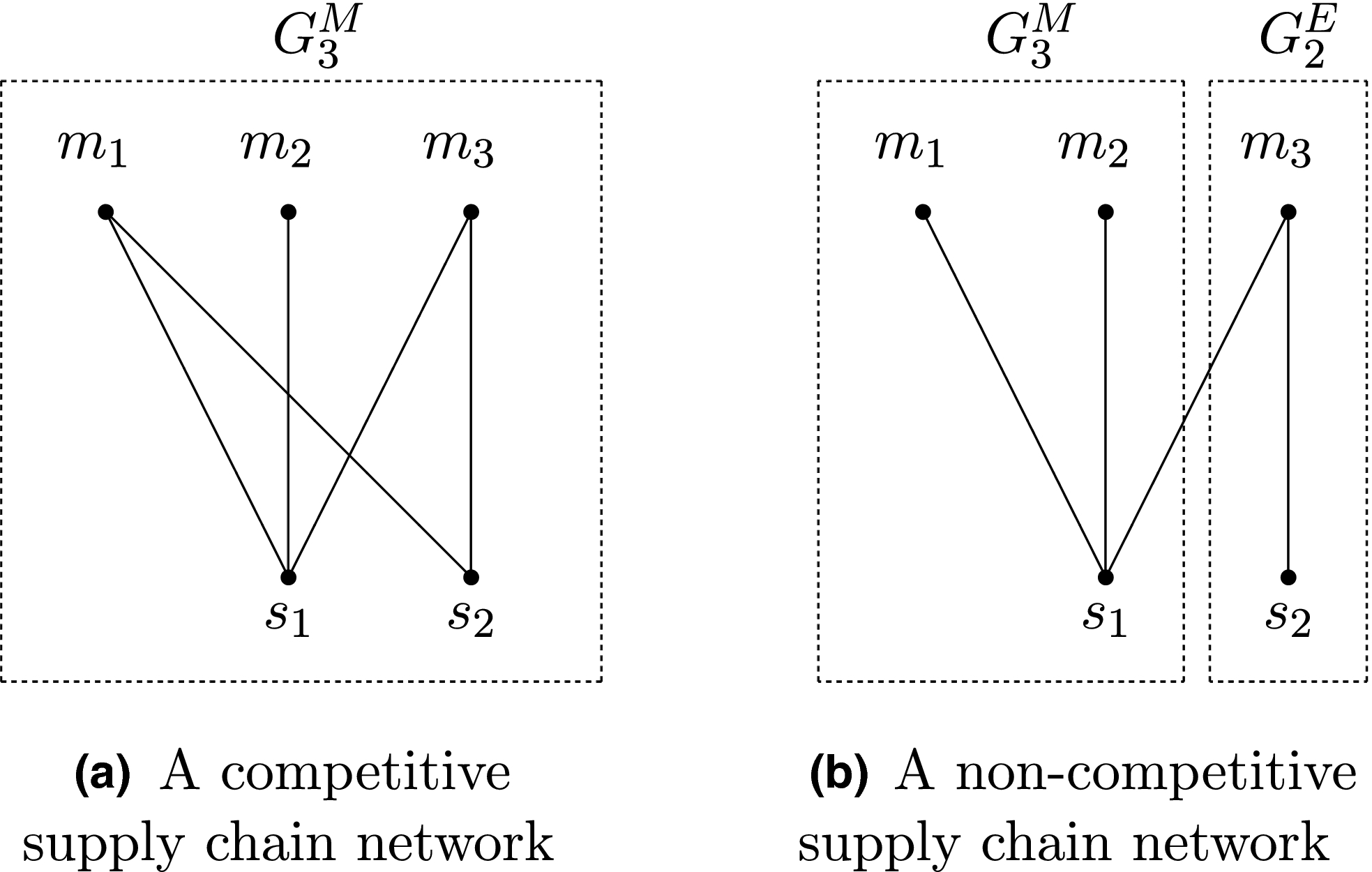
Competitive vs. Non‐Competitive Supply Chain Networks

Proposition 5

An efficient supply chain network may not be competitive whereas a competitive supply chain network must be efficient.

Proposition 5 implies that the conditions for a competitive network are more restrictive than conditions for an efficient network. We show in the appendix that a supply chain network is competitive if and only if it decomposes into subnetworks of a unique type so that all trades take place at the same price. If it only decomposes to

G_{k}^{E}

or G ^S types of subnetworks, the supply chain network must be efficient too because all manufacturers in these two types of subnetworks will be able to trade. If the network only decomposes to

G_{s}^{M}

type subnetworks, the only manufacturers that cannot obtain a good in the equilibrium are soft manufacturers and therefore, only manufacturers with the highest valuations trade. However, an efficient network, where manufacturers with the highest valuations trade, may not be competitive because these manufacturers may trade at different prices in equilibrium. Therefore, there could exist a divergence between the efficiency of a network, which is a network level concern, and the competitiveness of a network, which is a firm level concern.

Incomplete Information on Network Structure

In our setting, a firm's bargaining power depends not only on the number of his business partners but also on the identities and bargaining power of his partners. Each partner's bargaining power depends in turn on the strengths of his corresponding partners, and so forth. This implies that an adequate measure of bargaining power needs to reflect the global supply chain network structure. Therefore, we assume that the network structure (G, v) is common knowledge to all firms on the supply chain network. As we have discussed before that this is a strong, but necessary assumption to our model. This assumption would fit some industries (e.g., with limited number of dominant players) than others (e.g., fragmented industries with large amount of firms) in which firms would have incomplete information about network structures.

Our model can be extended to capture some forms of incomplete network information assumption. For example, the simplest form of incomplete network information would be the case where there is symmetric uncertainty regarding the graph structure (i.e., firms are all equally uncertain and agree upon the respective probabilities). In this case, firms simply face the expected value of the possible games. To illustrate, let

G

be the set of all bipartite graphs. Let F be the probability distribution function over

G

. We know from Proposition 2 that there exists a unique equilibrium (in terms of payoffs) for each

G \in G

. Let

p_{i}^{G}

be the equilibrium strategy of firm i in graph G. Then,

E [p_{i}^{G}] = \sum_{G \in G} p_{i}^{G} F (G)

would represent the equilibrium strategy of firm i when the firms are not certain about the graph structure. Then, the equilibrium payoff for the manufacturer with valuation v _i would be

v_{i} - E [p_{i}^{G}]

and the equilibrium payoff for a supplier would be

E [p_{i}^{G}]

A relatively more practice oriented approach would require a model with asymmetric information regarding the graph structure. In the ideal case, firms may have knowledge about their own links but not about their neighbors’ links. Such a model requires that each firm i has a different probability distribution function

F_{i} = F (G | L (i, G))

defined over

G

where L(i, G) is the set of links that contains firm i in graph G. This implies that the bargaining game is not a Bayesian game since the probability distribution over the set of bargaining games is not common knowledge. In other words, a tractable Bayesian model of networks would require a common prior for all firms’ beliefs about the network structure (i.e., F _i = F _j for all i and j), which implies that the model should be ex ante symmetric. The ex‐ante symmetric models would not coincide with our model's purpose of studying the impact of valuation heterogeneity among manufacturers agents since the identities of the neighbors are at the core of our model.

In summary, a relaxation of complete information assumption on the graph structure, which has potential to generate interesting and novel insights, would be desirable, however, such a model would be technically challenging and beyond the scope of this study.

Conclusion

This paper studies bargaining between manufacturers and suppliers in a supply chain network where firms must have an established business relationship or “link” to bargain and trade. The network structure of a supply chain restricts the equilibrium trading pattern in the network. We model such a supply chain via a bipartite graph. Through this model, we examine how supply and demand balance, network structure, and valuation heterogeneity among manufacturers jointly influence the equilibrium prices and trading pattern of the supply chain networks.

We have shown that valuation heterogeneity among manufacturers plays an important role in interacting with supply and demand balance and network structure of a supply chain network to influence the equilibrium outcome of the supply chain network. Valuation heterogeneity among manufacturers serves as a counter force to unfavorable supply and demand imbalance to protect the manufacturers from surplus extractions by the suppliers. Therefore, whether a supplier can get a good deal in the bargaining in a supply chain network not only depends on how many manufacturers he has a link with, but also depends on the quality of the manufacturers (in terms of valuations) he has a link with. We also found that bargaining actually takes place in smaller subnetworks in a general supply chain network as firms may selectively bargain with a subset of firms with whom they are linked. In other words, firms may ignore some of their links in the network that are not useful for them to get a better deal. We develop a decomposition algorithm to identify these subnetworks in which bargaining between firms will effectively take place in general supply chain networks. This implies that a firm should select the right set of firms on the other side of the supply chain network with whom it has a link to bargain in order to get a good deal.

For a supply chain network to be efficient, only the manufacturers with the highest valuations can trade. We found that both the network structure and identities of firms that hold key positions in the network matter to characterize the set of efficient networks. Adding a new link into a supply chain network can improve its efficiency if with the new link, more trades can happen in the network or manufacturers with higher valuations can replace manufacturers with lower valuations to trade in the network. We also demonstrate that the conditions required to make a supply chain network competitive are quite different from the ones to make the network efficient. Our results suggest that there could exist a divergency between competitiveness, which is a firm level concern, and efficiency, which is a network level concern, of a supply chain network.

There are several potential extensions of our research. We could consider the case where suppliers are asymmetric in terms of their costs. It is interesting to see how the asymmetries on both sides of the network impact the equilibrium outcome of the network. We can relax the assumption on unit demand and supply to consider the case where each supplier can supply more than one unit of the component and each manufacturer can buy more than one unit of the component. Another interesting extension could be the impact of uncertainty of supply and demand on the equilibrium.

Footnotes

Acknowledgments

The authors thank the senior editor, and two anonymous referees for valuable comments and suggestions.

1

For any finite set X, |X| represents the number of elements in X.

2

See Lóvasz and Plummer (), for more details on the Gallai‐Edmonds decomposition of graphs.

References

Abreu

Manea

. 2012. Bargaining and efficiency in networks. J. Econ. Theory 147(1): 43–70.

Acemoglu

Dahleh

M. A.

Lobel

Ozdaglar

. 2011. Bayesian learning in social networks. Rev. Econ. Stud. 78(4): 1201–1236.

Adida

DeMiguel

. 2011. Supply chain competition with multiple manufacturers and retailers. Oper. Res. 59(1): 156–172.

Ashlagi

Kanoria

Leshno

J. D.

. 2017. Unbalanced random matching markets: The stark effect of competition. J. Polit. Econ. 125(1): 69–98.

Belavina

2018. Supply networks for relational sourcing. Working paper, University of Chicago, Chicago, IL.

Bernstein

Federgruen

. 2005. Decentralized supply chains with competing retailers under demand uncertainty. Management Sci. 51(1): 18–29.

Bimpikis

Ehsani

Ilkilic

. 2018a. Cournot competition in networked markets. Management Sci. Forthcoming.

Bimpikis

Fearing

Tahbaz‐Salehi

. 2018b. Multisourcing and miscoordination in supply chain networks. Oper. Res. 66(4): 1023–1039.

Bloch

Querou

. 2013. Pricing in social networks. Games Econ. Behav. 80: 243–261.

10.

Cachon

G. P.

Lariviere

M. A.

. 2005. Supply chain coordination with revenue‐sharing contracts: Strengths and limitations. Management Sci. 51(1): 30–44.

11.

Candogan

Bimpikis

Ozdaglar

. 2012. Optimal pricing in networks with externalities. Oper. Res. 60(4): 883–905.

12.

Chen

Sun

Tang

Wang

Zhu

Z. A.

. 2011. Optimal pricing in social networks with incomplete information. International Workshop on Internet and Network Economics, 49–60.

13.

Cohen

Harsha

. 2018. Designing price incentives in a network with social interactions. Manuf. Serv. Oper. Manag. Forthcoming.

14.

Corbett

C. J.

Karmarkar

U. S.

. 2001. Competition and structure in serial supply chains with deterministic demand. Management Sci. 47(7): 966–978.

15.

Corominas‐Bosch

2004. Bargaining in a network of buyers and sellers. J. Econ. Theory 115(1): 35–77.

16.

Elliot

2015. Inefficiencies in networked markets. Am. Econ. J.: Microecon. 7(4): 43–82.

17.

Feng

Lai

L. X.

. 2015. Dynamic bargaining in a supply chain with asymmetric demand information. Management Sci. 61(2): 301–315.

18.

Tong

. 2008. Contracting and information sharing under supply chain competition. Management Sci. 54(4): 701–715.

19.

Hsu

V. N.

Lai

Niu

Xiao

. 2016. Leader‐based collective bargaining: Cooperation mechanism and incentive analysis. Manuf. Serv. Oper. Manag. 19(1): 72–83.

20.

Huang

Gumus

Ray

Zhang

. 2016. United we stand, divided we fall: Strategic supplier alliances under default risk. Management Sci. 62(5): 1297–1315.

21.

Jackson

2008. Social and Economic Networks. Princeton University Press, Princeton, NJ.

22.

Kleinberg

Tardos

. 2008. Balanced outcomes in social exchange networks. Proceedings of the 40th ACM Symposium on Theory of Computing, May 17–20, 2008, Victoria, Canada.

23.

Kluberg

Perakis

. 2012. Generalized quantity competition for multiple products and loss of efficiency. Oper. Res. 60(2): 335–350.

24.

Kranton

Minehart

. 2001. A theory of buyer‐seller networks. Am. Econ. Rev. 91(3): 485–508.

25.

Lobel

Sadler

. 2015. Information diffusion in networks through social learning. Theor. Econ. 10(3): 807–851.

26.

Lóvasz

Plummer

M. D.

. 1986. Matching Theory. North‐Holland, Amsterdam.

27.

Lovejoy

W. S.

2010. Bargaining chains. Management Sci. 56(12): 2282–2301.

28.

Manea

2011. Bargaining in stationary networks. Am. Econ. Rev. 101(5): 2042–2080.

29.

Manea

2018. Intermediation and resale in networks. J. Polit. Econ. 126(3): 1250–1301.

30.

Martinez de Albeniz

Simchi‐Levi

. 2013. Supplier‐buyer negotiation games: Equilibrium conditions and supply chain efficiency. Prod. Oper. Manag. 22(2): 397–409.

31.

Nagarajan

Bassok

. 2008. A bargaining framework in supply chains: The assembly problem. Management Sci. 54(8): 1482–1496.

32.

Nagarajan

Sošić

. 2009. Coalition stability in assembly models. Oper. Res. 57(1): 131–145.

33.

Nava

2015. Efficiency in decentralized oligopolistic markets. J. Econ. Theory 157: 315–348.

34.

Netessine

2009. Supply webs: Managing, organizing, and capitalizing on global networks of suppliers. Kleindorfer

P. R.

Wind

Y. R.

Gunther

R. E.

, eds. The Network Challenge: Strategy, Profit, and Risk In an Interlinked World. Pearson Prentice Hall, Upper Saddle River, NJ, 225–241.

35.

Pasternack

B. A.

1985. Optimal pricing and return policies for perishable commodities. Market. Sci. 4(2): 166–176.

36.

Perakis

2007. The price of anarchy under nonlinear and asymmetric costs. Math. Oper. Res. 32(3): 614–628.

37.

Perakis

Roels

. 2007. The price of anarchy in supply chains: Quantifying the efficiency of price‐only contracts. Management Sci. 53(8): 1249–1268.

38.

Polanski

2007. Bilateral bargaining in networks. J. Econ. Theory 134(1): 557–565.

39.

Rubinstein

1982. Perfect equilibria of a bargaining model. Econometrica 50(1): 97–110.

40.

Spengler

1950. Vertical integration and antitrust policy. J. Polit. Econ. 58(4): 347–352.

41.

Chen

. 2010. Optimal control and equilibrium behavior of production‐inventory systems. Management Sci. 56(8): 1362–1379.