
Abstract
We study the merits and limitations of technology improvement (TI) initiatives for managing input–price risk. Such initiatives (e.g., energy efficiency projects) typically reduce the consumption of an input commodity and so result in lower production costs, more sustainable operations, and/or an improved competitive position. This study explores whether TI can also serve to hedge risks. Although TI clearly reduces both average cost and risk exposure, some firms may actually benefit from input–price uncertainty; the result, when combined with production flexibility, is an “option value” that firms may well be reluctant to forgo. We develop a stylized mathematical model to examine the incentives of different types of firms to adopt TI. Thus, we derive a closed‐form expression that quantifies a firm’s attitude toward input–price risk by considering the firm’s certainty premium, or what the firm would pay to “lock in” the unit input price, and then link that premium to various firm‐ and industry‐specific characteristics. We also compare the risk management advantages of technology improvement vs. financial hedging (FH) and give conditions under which these strategies are complements or substitutes. Our results show that, even when input‐price uncertainty is desirable for firms, they can still benefit from investing in risk reduction measures—such as TI and FH—because the uncertainty’s option value could thereby increase. A firm’s ability to adjust its price in response to both market competition and input‐price variation mediates the benefit of risk‐reducing measures and also affects the complementarity of these two strategies.
Introduction
Uncertainty in the price of input commodities is a major concern of any firm that relies on them for its production process. The variability of input prices has increased significantly (by as much as 50%) in the last two decades, with significant effects on firms’ operations and profitability (Manyika 2012). For instance, energy—which accounts for 30% of the cement industry’s operational costs—has seen considerable price variability in recent years (Thrall 2012). A construction company’s operational costs are directly affected by the price (and its variability) of primary construction materials, including cement and asphalt (Zhou and Damnjanovic 2011). Manufacturers of wind turbines and solar panels are also concerned about surges in the magnitude of, and uncertainty in, the price of industrial and rare earth metals (Shen 2012).
As a strategy for managing the operational cost of inputs, many firms invest in technology improvement (TI) projects—that is, technical changes that reduce the consumption of an input commodity needed for a given amount of output. For instance, “Delta Faucet […] saves 2.8 billion Btu in natural gas annually for heating the tanks as well as $2,000 per month in reduced chemical costs through changes to its degreasing process.” 1 In the energy‐intensive oil refinery industry, where the ratio of energy value, used to run the refining process, to value‐added varies between 10% and 25%, a frequently used TI measure is to implement “flare gas recovery” (FGR), which not reduces costs but also lowers emissions and thus air pollution.
Using TI to reduce the rate at which input commodities are consumed for the same amount of output can affect a firm’s profit in two ways. First, it has an average‐price effect by reducing the firm’s average unit operational cost. Second, TI also changes how input‐price uncertainty affects the firm’s profit risk by reducing the intensity of commodity use in both the production process and the total cost function. For example, “thanks to the efficiency project, [Delta Faucet] is less vulnerable to price volatility and better able to plan costs than if it had stuck with its prior process.” 2 Motivated by numerous examples of firms investing in TI projects, this study critically examines the incentives of firms to use TI for risk management purposes as an additional value on top of the conventional benefits.
Practitioners have long noted the value of TI as a risk management strategy. According to Treanor et al. (2013), “[a]n airline choosing to operate a newer, more fuel‐efficient fleet has less exposure to the price of jet fuel.” A report by Chatham House (2011) suggests that “reducing energy consumption lowers the exposure of companies to volatile energy prices, making their profits more secure and lowering the risk of their defaulting on loans.” 3 Technology improvement is thus viewed as an initiative that firms can incorporate into their overall risk management strategy.
Despite the practical potential of TI as an operational risk management strategy, that aspect of TI has not received much attention in the academic literature. Technology improvement, in the sense that we discuss here, neither fits into any of the operational risk management categories classified by Van Mieghem (2011), nor is also not included in the six major categories of operational risk management given by Zhao and Huchzermeier (2015). To the best of our knowledge, this study is the first formal examination of TI’s risk management benefits and of firms’ incentives to use it for that purpose.
However, a firm seeking to invest in TI as a risk management measure is faced with a critical trade‐off. On the one hand, a firm’s risk aversion motivates its investment in all risk‐reducing measures, including TI. On the other hand, it is well known that firms may benefit from input–price uncertainty provided that their profit function is convex with respect to the uncertain parameter (Cabral 2003, Oi 1961). The analytical explanation for this phenomenon is that, for a convex profit function, such uncertainty creates an embedded “option value.” In practice, this means that a firm is able to adjust its production levels asymmetrically in response to fluctuations in the price of inputs: reducing (resp. increasing) production levels when that price is high (resp. low), thereby endogenously creating a convex payoff (see Goyal and Netessine 2011, Plambeck and Taylor 2013). Alexandrov (2015) extends this insight to the case of competition under certain conditions. The implication is that, under those conditions, firms may benefit from deliberately exposing themselves to input–price uncertainty. So the firms’ response to input‐price uncertainty is driven not only by its attitude toward risk but also by the profit function’s structure. What makes the trade‐off just described especially interesting for technology improvement is that TI changes the structure of the firm’s profit function (viz., its convexity) in a fundamental way, which brings up the following research question: Under what conditions do firms benefit—from a risk management perspective—from investing in technology improvement? To answer this question, we explicitly derive the “certainty premium” that firms are willing to pay for a riskless input price as a function of four factors: the extent of uncertainty, the profit function’s curvature, the risk aversion parameter, and the total amount of commodity inputs used in the firm’s operations. We then analyze the effect of investing in TI on this certainty premium under various conditions. This approach has the advantage of allowing us to isolate the risk management properties of TI while controlling for the average‐price effect, which is driven instead by the focal technology’s cost effectiveness. 4
Technology improvement is seldom the first option that comes to mind when considering strategies for the management of input–price risk. Companies in various industries have long deployed an array of different risk management strategies to shield themselves from input–price volatility. Financial hedging (FH) is the most common risk management strategy used by firms (Froot et al. 1993) in most industries. Yet FH instruments do have some limitations, of which the most important is that contingent claim contracts may not exist for the commodities of interest. In these cases, a firm must resort to using the most closely related futures contract available in the market and thus can achieve only a partial hedge—as when airlines use crude oil or heating oil futures and options to hedge jet fuel price risks (Adams and Gerner 2012). Furthermore, FH instruments cannot fully cover a firm’s exposure to production risks or demand quantity risks (Moschini and Lapan 1995). As a result of these limitations, TI becomes an important complement or even substitute to FH for managing input‐related risks. However, FH and TI are fundamentally different when it comes to production economics. While an FH instrument typically reduces an input’s price volatility but not its mean, TI reduces both mean and volatility, thus affecting profit function’s curvature (and hence the option value of uncertainty). Our model provides insights into the relative merits and drawbacks of each strategy vis‐à‐vis input–price uncertainty, and it also enables investigating the conditions under which FH and TI strategies are complementary.
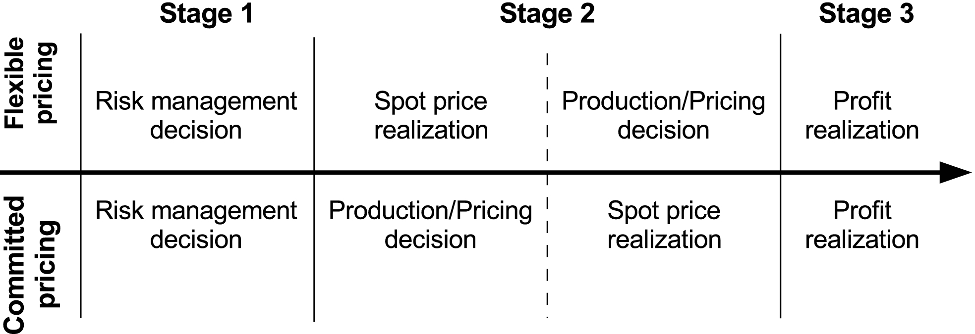
In order to better explain the incentives for investing in TI, we characterize the circumstances under which a firm’s profit function is convex in the input price. The flexibility in choosing the production plan before or after the realization of uncertainty is one the key determinants of the convexity. In some industries, firms have the flexibility to adjust their production plan or price after observing the realizations of uncertain input costs. In the shipping industry, for example, companies can adjust their freight rates in response to realized fuel costs (Wang and Lutsey 2013). In other industries, the market is committed to a price long before production actually occurs; thus firms must decide on a price plan before observing the realization of input–price shocks. For instance, airlines offer tickets several months before the flight even though the price of jet fuel changes almost daily (Morrell and Swan 2006). Moreover, industry characteristics (e.g., the level of competition) also affect the structure of a firm’s profit function, which in turn affects attitudes toward input–price uncertainty and investment in TI. Table 1 summarizes and provides examples of the scenarios we examine for firms characterized by low vs. high aversion to risk.
Interaction between Industry and Firm Type (RA↑, high risk aversion; RA↓, low risk aversion)
Our results suggest that if a firm has access to fair and efficient FH for its input(s), 5 where the transaction cost of hedging is minimal, then FH will be predominant in the firm’s risk management strategy. This is because while FH does not alter the structure of production function, TI reduces the convexity of the profit function, and hence the embedded flexibility option. Furthermore, firms can remove all of input price uncertainty by implementing FH. TI, however, can only partially remove this uncertainty, although providing the firm with the average cost reduction benefit. Thus, flexible firms find it optimal to use FH if the transaction costs associated with FH is not too high.
However, if FH is not available or is too costly (due to factors such as transaction costs, liquidity problems, spot–futures mismatch, and administrative costs), then TI is sometimes an adequate substitute. Absent FH, firms with a committed production technology will choose TI to manage input‐price risk because they are not concerned with the impact of TI on the convexity of profit function; also firms with a flexible production technology will consider TI, but only if their aversion to risk is above a certain threshold to justify the reduction in the flexibility option value. The TI and FH risk management strategies can be complements or substitutes depending on three factors: the firm’s level of risk aversion, its ability to adjust prices in response to changing input prices, and the extent of competition in the market. In particular, the two strategies become complement when a firm benefits from the risk reduction effect of FH while enjoying the average cost reduction benefits of TI. Our results also suggest that, if a firm faces demand uncertainty in addition to input–price uncertainty, then it has more (resp. less) incentive to invest in TI when input price and demand are positively (negatively) correlated. By creating additional convexity in the profit function, demand uncertainty may increase the flexible firm’s interest in implementing TI if that uncertainty is positively correlated with input‐price uncertainty.
Literature Review
The main distinguishing feature of this study is its analysis of firms’ incentives to invest in technology improvement—not only to reduce costs and ensure sustainability but also as part of a risk management program. Thus, we contribute to research that addresses the interface between operations management and finance. Our study is related to previous theoretical work that focuses on the relative merits and complementarity of operational hedging and tools for managing financial risk (for reviews see Birge 2014, Van Mieghem 2003, 2011 and Zhao and Huchzermeier 2015). The papers in that stream of the literature fall into two broad areas within operations management (OM): (i) inventory order policies and (ii) capacity management and technology choice.
Research in the first category examines inventory risk management and studies the impact of financial hedging on optimal procurement and ordering policies. Starting with the seminal work of Gaur and Seshadri (2005) and Chen et al. (2007), the optimal hedging of inventory risk has been extensively discussed in the OM literature. The main focus of this literature is on using financial instruments to reduce the “mismatch cost” between supply and demand (Devalkar et al. 2018, Kouvelis et al. 2018, Park et al. 2017, Turcic et al. 2015). In addition to the obvious contrast of context and applicability, our study differs from those just cited with regarding to timing. More specifically: TI is a one‐time investment that reduces the firm’s exposure before spot prices are realized; whereas a FH instrument (or a purchase contract) that compensates for the firm’s possible losses after the realization of random costs.
Closer to our work is research in the second category, which examines ex ante policies of operational or technology investment. These investment policies encompass such “embedded” real options as decentralization, production postponement, and production flexibility. Apart from a large number of empirical studies (see e.g., Allayannis et al. 2001) with only limited relevance to our work, theoretical research on this topic has received an increasing amount of attention in the OM literature (Chen et al. 2014, Chod et al. 2010, Ding et al. 2007, Huchzermeier and Cohen 1996). Most of this work focuses on the benefits of adding capacity flexibility—a form of technology improvement that differs from what we study—when demand is uncertain (for a review, see Boyabatli and Toktay 2011). Goyal and Netessine (2007) identify the optimal level of investment in two rival technologies (a product‐flexible technology and a product‐dedicated technology) and Chod et al. (2010) consider an extension to that model that incorporates a postponement option. In Ding et al. (2007), supply flexibility is created by deciding on offshore vs. domestic capacity investment under exchange rate risk; in Wang et al. (2010), supply flexibility arises instead from supplier diversification. Dong et al. (2014) characterize the value of conversion flexibility for managing input and output shocks. All these studies can be categorized within Hopp’s (2011) framework for operational strategies of risk management, yet apparently none of them consider TI as a risk management strategy. Our notion of technology improvement is actually identical to Plambeck and Taylor’s (2013) “input efficiency.” Those authors explore the trade‐offs, in the context of risky input and output prices, among investing in input efficiency, investing in capacity improvement, or adopting a “flexibility option.” However, their paper considers neither the firm’s pricing decisions nor the possibility that financial hedging could serve as a risk management strategy.
As for the finance side of the OM–finance interface, a number of scholars (e.g., Baron 1970, Hartman 1976) have studied the behavior of firms facing uncertain input/output prices. Sandmo (1971) and Batra and Ullah (1974) add risk aversion to the behavioral model of a firm that is producing under input–price uncertainty and that must also conform to a production plan determined ex ante. Turnovsky (1973) and Epstein (1978) highlight the critical role of flexibility in adjusting a production plan before or after realization of the random shock. Another group of papers (including Moschini and Lapan 1992, Viaene and Zilcha 1998) consider the roles of production flexibility and optimal production decisions in the presence of random input/output prices and hedging instruments. More recently, Alexandrov (2015) see also the citations therein) demonstrates that firms benefit from exposure to risk if they can make adjustments after observing the realization of a random production parameter. Assessing the benefits of financial hedging in practice, 6 Alexandrov describes the conditions under which hedging is not a profitable strategy by addressing the value of uncertainty when the profit function is convex with respect to the uncertain parameter (here, input price)—a convexity that stems from Jensen’s inequality. Our own study is similarly based on analyzing (i) the profit function’s convexity with respect to input price and (ii) the effect of TI investment on the profit function. We find that if hedging is not a profitable strategy then TI investment may be a viable substitute. In addition, we extend the analysis by accounting for firms’ relative flexibility regarding a price commitment.
In sum, our work complements the existing OM–finance literature and offers novel contributions in some important respects. We propose TI as a potential risk management strategy and study firms’ incentives to adopt it, especially in the presence of FH. This study shows how the theoretical results of Alexandrov (2015) and Oi (1961) can be applied to help us better understand the TI investment trade‐offs between reducing exposure to risky input prices and losing the beneficial convexity of the profit function. We derive a simple and intuitive explicit measure of the certainty premium for risky inputs—a measure that accounts not only for profit convexity but also for the firm’s internal and external characteristics. Finally, we study how competition and market power affect the interaction between financial hedging and TI investment.
Modeling Input–Price Uncertainty
Our basic setup involves a monopolistic, risk‐averse firm that produces a homogeneous product sold at price p in a single market. We consider a linear demand function q(p) = a − bp for a the market size and b the sensitivity of demand to price. The per‐unit production cost 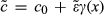


The Timeline: Flexible vs. Committed Firms
There are two stages of decision making. In the first stage, the firm decides on its level of investment in technology improvement. In the second stage, the firm makes its production decision—that is, it sets the output price and thus the quantity to be produced.
As illustrated in Figure 1, we study two different setups in the second stage. In the first (resp. second) setup, the pricing or quantity decision occurs after (resp. before) resolution of input–price uncertainty. The difference between these two timelines reflects the firm’s ability to adjust its production decisions after realization of the input price. In that case, the firm chooses a product price such that the input‐price shock is transferred (in full or in part) to the consumer; we refer to this setup as the flexible case. In contrast, if the firm sets the output price before the input price is realized (as occurs under the long‐term contracts typical of many value chains), then the firm cannot adjust its product price. This setting is known as the committed case. 9 These two timelines affect firms’ TI investment decisions in different ways, as we describe in section 4.
Timeline of Events
Note that, for flexible and committed timelines both, the decision on TI investment occurs before realization of the input price; this timing means that the firm’s expected profit/utility is maximized in Stage 3. Now taking into account the TI investment expenditure, x, we can write the firm’s profit as 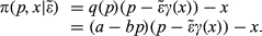
Price Optimization Problem: The Flexible Firm. In the flexible setting, the firm chooses—for a fixed level of TI investment—a market price 
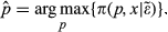
Price Optimization Problem: The Committed Firm. In the committed setting, pricing decisions must be made before uncertainty is resolved. So in this scenario, the second‐stage optimization problem becomes 


Determinants of Firms’ Attitudes Toward Input–Price Risk
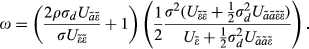
Input‐price risk is not always undesirable, even for a risk‐averse firm. To understand this seeming anomaly, consider a firm that purchases an input commodity at price 


(a) Assume that the firm is risk neutral. Then, for a flexible (resp. committed) firm with a positive production quantity, (b) The certainty premium ω can be approximated as


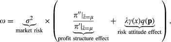


Given Jensen’s inequality, 11 a crucial implication of Lemma 1(a) is that a risk‐neutral flexible firm does benefit from the input cost’s randomness. As mentioned in the Introduction, this counterintuitive result is well known in the literature (Oi 1961). The idea is that the profit function’s convexity in the input price gives a firm the option to expand production during favorable times (i.e., when inputs are cheap) and to contract production in unfavorable times (when inputs are expensive). Part (b) of the lemma helps explain the factors that drive a firm’s attitude toward input‐price risk, which we now discuss in turn.
Market Risk. The effect of 
Profit Structure. The profit function’s structure figures prominently in the firm’s attitude toward input–price uncertainty. One important factor is whether the firm is flexible or committed in its pricing decision. In particular, if one considers part (a) of Lemma 1 then 
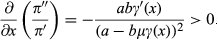
To assess the marginal risk management value of TI, we need only look at how TI investment affects ω—that is, at 

To do so, we begin by exploring how TI investment influences the profit structure effect. In the committed setting, where 

Risk Aversion. Lemma 1(b) extends the result in part (a) to explain why it is not only risk‐neutral firms that desire input‐price uncertainty.
The firm’s overall risk attitude, which is represented by the certainty premium ω, is determined by two opposing effects: that of the firm’s profit structure and that of its attitude toward risk. Therefore, a risk‐averse firm might want to invest in TI for purposes of risk management. Yet if the firm is not very risk averse and so the profit structure effect prevails, then the firm might have a relatively favorable attitude toward input‐price risk.
For flexible firms, the effect of TI investment levels on its risk management value (i.e., on 
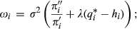
Quantity of Input Used. Recall that, for a fixed technology level x, we use γ(x)q(
Technology improvement changes both the curvature of the profit function and the quantity of input used. 12 The latter is the main difference between financial risk management (e.g., via hedging) and TI measures: FH never affects the quantity of input used and so cannot affect the firm’s certainty premium directly (i.e., by changing input quantities)—except, as we show in section 5, in a competitive setting.
Options for Managing Input‐Price Risk
As previously discussed, technology improvement can significantly affect the value (for a firm) of input–price uncertainty. Furthermore, the availability of financial risk management mechanisms should affect a firm’s risk preferences and thus its view on input–price uncertainty. In this section, we explore these effects for the two strategies and compare them from the perspective of risk.
Investment in Technology Improvement
Technology improvement affects the total amount of input commodity used and also the profit function’s curvature. Here, we consider the amount of TI investment as a decision variable and examine its relation to input–price uncertainty.
The firm’s Stage 1 optimization problem (cf. Figure 1) regarding TI investment is 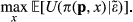
For a flexible firm: (a) ω increases with x if and only if (iff) For a committed firm: (c) ω decreases with x iff 


All proofs are given in Appendix C.
To explain the intuition behind part (a) of the proposition, recall the two notable effects of increased investment (x) on the firm’s profit function. From Equation 6 (in Lemma 1(b)) it is clear how these two opposing forces determine the firm’s certainty premium ω. If λ is low, then the option value is more important to the firm; that is, the firm increasingly prefers to seek input‐price uncertainty. So when investment reduces uncertainty, the certainty premium always increases with such investment. Yet for firms that are sufficiently risk averse, the risk attitude effect—a combination of risk aversion and input use quantity as presented in Equation 6—dominates. Given that 
Part (b) of Proposition 1 is a direct consequence of part (a). Technology improvement reduces the mean and the variance of input used. Greater variance in the input price does not change the expected use, but it does increase the risk associated with input price. With reference to part (a), we can see that if λ is low (resp. high) then the firm seeks to increase (resp. decrease) input‐price uncertainty; therefore, the firm invests less (resp. more) in TI as variance increases. See Panel (a) of Figure 2. Thus a risk‐neutral flexible firm reduces its TI investment in response to increased uncertainty. At the limit, if input–price uncertainty is extremely high then TI investment may be deemed unprofitable. The thresholds for λ in part (a) and (b) differ only because of the approximate nature of mean–variance preferences. Numerical results indicate that those thresholds are fairly close to each other: 

Investment in Technology Improvement [Color figure can be viewed at
The main difference in the case of a committed firm is that its profit function is linear with respect to (w.r.t.) the input price (cf. Lemma 1); as a result, the first term in Equation 6 is eliminated. In other words, input–price risk no longer has any option value. When 


These results hint at an important feature of TI investment: risk‐averse firms can use it as a tool for managing risk. Indeed, decreasing the value of a random variable decreases both its mean and its variance. If the firm prefers input–price variance because of the associated option value, then TI loses its value. But if the firm is risk averse and would prefer to avoid input‐price risk, then TI is a good way to manage that risk and also to reduce the average price.
In practice, firms’ incentives for investing on TI are also strongly dependent on such factors as the input commodity’s cost “intensity”—related to magnitude of γ(x)—(i.e., whether the input cost accounts for low or a high percentage of production/operations costs) and investment effectiveness (the amount of saving per each dollar of TI investment). In section 6, we build a general framework to accommodate the effect of these factors in the model.
Financial Hedging
Financial hedging is a conventional option for managing input‐price uncertainty. The availability of FH mechanisms (futures contracts or options) to manage input risk directly affects the firm’s pricing decision, its attitude toward input‐price variation (which we proxy by the certainty premium ω), and its utility. So in this section, we consider a setting where, in Stage 1, the firm can adopt both strategies.
When hedging is available, the net profit of a firm in Stage 3 will be the sum of returns from operational activity and from hedging: 

In a fair hedging contract, 


The optimal hedging positions and the optimal prices for the flexible and committed settings are as follows. In the flexible setting, Finally,

According to part (a) of this proposition, it is optimal for a risk‐averse firm—irrespective of its pricing flexibility—to devise a hedge against all of the input commodity used (i.e., against γ(x)q(
Certainty Premium in the Presence of Financial Hedging. The following lemma extends the results of section 3.2 to the case where financial hedging is a viable option.
The possibility of setting up a hedging position does not affect the option benefit that follows from the profit function’s convexity. However, FH availability does influence the risk attitude effect for firms that are risk averse. A risk‐neutral firm is neither better‐ nor worse‐off after making a fair hedge. This finding augments the results of Alexandrov (2015) by including risk‐averse firms—though with a low level of risk aversion—with risk‐neutral firms in terms of preferences for exposure to risk. The main difference here is that FH tends to increase risk‐seeking behavior by rendering ω even more negative.
Hedging Via Financial Instruments vs. Investing in Technology Improvement
Risk Management Perspective. An immediate consequence of Lemma 2 is that financial hedging reduces the certainty premium. Thus, hedging allows firms to enjoy greater benefits from the input price’s uncertainty if the level of risk aversion is low. The reason is that FH reduces the volatility of total cash flow but without affecting the beneficial convexity of the profit function. This result contrasts with the effect of technology improvement, which can either increase or decrease ω (see Proposition 1).
Quantifying the certainty premium for firms that engage in TI vs. FH allows us to compare the two strategies strictly from the risk management perspective—that is, without considering the average‐price effect mentioned in the Introduction. Our next proposition will prove useful in comparisons, from this risk management perspective, between the case of hedging without TI investment (h =
In the flexible setting, 

For both the flexible and committed settings, the optimal hedging position is chosen so as to minimize the firm’s certainty premium; indeed, the certainty premium under optimal hedging is lower than the premium under optimal TI investment. In the flexible setting, the optimal hedging position removes the effect of input quantity used; hence there remains only the negative effect of profit structure, which reduces TI. In the committed setting, the effect of profit structure is zero (


Firm’s Utility Perspective. A comparison of the firm’s utility under a fair hedging position with its utility under a non–budget‐neutral TI investment (that also leads to an average cost reduction) would disadvantage financial hedging and therefore may not be meaningful. This is why we use the firm’s certainty premium to compare the risk management properties of these two solutions. However, our numerical experiments reveal that hedging’s certainty premium advantage might also outweigh the cost reductions due to TI. Figure 3 illustrates that, in the comparison between budget‐neutral TI and fair FH, the latter always yields a greater risk management benefit. When TI is not budget neutral, the risk management benefit increases with uncertainty. Therefore, there is some point at which the value of hedging exceeds the cost reduction benefits of non–budget‐neutral TI.

Normalized Difference between Expected Utilities in Budget‐Neutral TI and Fair FH in Flexible and Committed Settings [Color figure can be viewed at
Possible costs associated with FH motivate the use of TI as an efficient alternative for risk‐management purposes. If the cost is sufficiently high, then TI may always dominate FH. In this case, the pay‐off of the financial hedging changes to 

Technology Improvement and Financial Hedging: Substitutes or Complements?
Next, we discuss whether the value of investment in one strategy—in terms of expected utility—decreases or increases with more investment in the other option. Formally, we are interested to see whether TI and FH are substitute or complement options for the firm. The following proposition addresses this question.
In the flexible setting, TI and FH are always substitutes. In the committed setting, there exists a


This proposition considers both the cost reduction and certainty premium effects of TI. It suggests that the effect of hedging on a firm’s expected utility can always be replicated by substituting TI; in the committed setting, however, if the firm is sufficiently risk averse then the two strategies are complements. Proposition 2 helps to explain this effect by indicating that, in both flexible and committed settings, the optimal h falls as x rises. Since the optimal quantity in the flexible setting is independent of h, it follows that the effect of h on expected utility is moderated by the decreasing effect of x on h; hence we conclude that these two strategies are substitutes. Yet the optimal price is a function of h in the committed setting (see Proposition 2(b)) and so the effect of h on the firm’s expected utility could also be moderated by the optimal price, resulting in a more complicated dynamic. A highly risk‐averse firm chooses a cautious production plan to minimize volatility in the realized revenue. By reducing the disutility of volatile revenue, FH allows the firm to take advantage of the cost‐reducing effect of TI and increase its production level. The additional risk mitigating effect motivates the firm to invest more in TI which in turn results in a higher level of production, demanding a larger FH level. Thus, the two strategies become complement. This dynamic does not appear under low risk‐aversion because the dis‐utility of volatile revenue is already negligible.
Duopoly
Market competition affects the capacity of an individual firm to set the output price. In many situations, competition mitigates the value of existing options because the actions of rival firms reduce the focal firm’s ability to harness those options. We examine this generalization in the case of TI investment by comparing the incentives of firms operating in monopoly and duopoly markets. We begin by observing that a monopolist firm’s profit margin depends critically on its own decisions whereas, in highly competitive industries, the profit margin is determined by aggregate market forces and so is usually much less volatile than the margins of a monopolist firm. 16 It is therefore reasonable to assume that market competition has implications for the effectiveness of both operational and financial hedging as means to reduce the risk exposure of firms (Shaffer 1982). Scholars have argued that this interaction is fairly complex (see e.g., Caldentey and Haugh 2009).
Competition affects the firm’s costs and benefits associated with input‐price uncertainty by (i) changing the profit function’s curvature and (ii) changing the optimal output quantity and hence the total input commodity to be used. In this section, we consider competition between two firms; both of them have access to financial hedging, but only one invests in technology improvement. Our goal is to identify the competitive (dis)advantages of TI investment in a strategic environment.
Game Setup
Our model assumes a duopoly Cournot competition (on quantity) between two risk‐averse firms. The timeline of decisions is illustrated by Figure 1 (in section 3). The TI decision, and afterwards, the FH decision occur in Stage 1, and the production decisions are made in Stage 2; profits are realized in Stage 3. The output is a homogeneous good, and there is a single market price. The quantity supplied by each firm (

In Stage 2, the firms simultaneously decide about their optimal quantity. Firms in the flexible (resp. committed) case make production decisions after (resp. before) the random input costs are realized.
17
Formally, we have 

Flexible Firms
Denote the profit of each firm by 

Recall from Equation 6 that, in the monopoly setting, the first term related to the profit curvature is always negative. So were it not for the effect of risk aversion (introduced in the second term), the firm would always benefit from input‐price uncertainty. However, this generalization does not hold in the competitive setting. Lemma 3 shows in particular how, under duopoly, that first term can be either positive or negative—a dynamic that clarifies the effect of technology improvement.
The following proposition—whose claims are illustrated by the graphs in Figure 4—characterizes the optimal hedging positions and expresses formally how competition changes a firm’s attitude toward input‐price uncertainty.
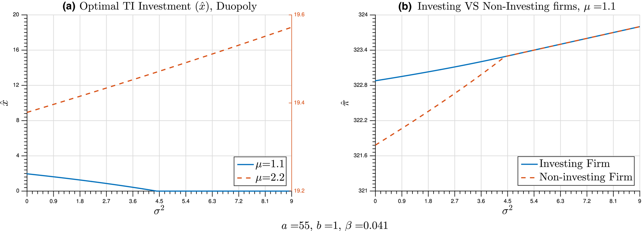
Duopoly Setting: TI Investment with Flexible PRICING [Color figure can be viewed at
Technology improvement is a substitute for financial hedging.
There exists a


Part (a) of this proposition suggests that, similarly to the monopolistic case, TI and FH are substitute strategies for managing input‐price risk. As before, this follows because the pricing decision is independent of the hedging position, where the latter is a decreasing function of x. Thus more investment results in h having less of an effect on expected utility.
There is a contrast with part (b), however. Unlike the monopoly setting, in which the optimal hedge is equivalent to using the optimal input quantity at any level of x, it is never optimal for the investing firm to hedge against all of its input commodity use. In fact, even without investment (γ(x = 0) = 1) the firm optimally hedges just two thirds of the input quantity used, since part of the expected profit is due to its rival’s quantity and hedging decisions. At the optimal hedging position, the effect of input quantity used disappears and so financial hedging further increases the firm’s benefit from input‐price uncertainty; that is, hedging eliminates uncertainty’s “negative” effects (those due to risk aversion) but retains its “positive” effects.
Part (c) of Proposition 2 suggests that γ(x) < 1/2 if and only if 


Committed Firms
Given the optimal production quantity and the hedging position that maximizes a firm’s expected utility, the optimal TI investment decision in Stage 1 is derived by solving 

According to Lemma 4, the profit curve’s convexity has no effect on the certainty premium in this setting and, moreover, the firm’s attitude toward risk is determined solely by the input quantity used.
α(x) is decreasing in x.

In light of Lemma 4, Proposition 6 shows that—in contrast to the flexible setting, where 


Extensions
In this section, we extend our analysis to study the effect of various factors that affect the risk management properties of TI. We also examine the effect of demand uncertainty and its correlation, in the model, with input price.
Sensitivity Analysis
In practice, there are several factors that might affect a firm’s decision to invest in TI and thus alter TI’s risk management properties. One example is the cost intensity of the input commodity—that is, the percentage of a firm’s production/operations cost for which the input cost accounts. Another example is TI investment effectiveness, or the amount of savings generated by each dollar invested in TI. In this section we extend our framework to assess the effects of these parameters.
Let γ(x; β) represent the unit input consumption function that is affected by an exogenous parameter β.
The firm’s optimal investment value
If γ(x; β) is supermodular then the effect of an extra unit of investment on reducing the input commodity’s use increases with β; this increase occurs in response to a higher optimal TI investment. Conversely, if γ(x; β) is submodular then the same extra unit’s effect decreases with β, which implies a lower level of optimal TI investment.
We can now use Lemma 5 to characterize how the effect of β on TI’s risk management properties depends on the submodularity or supermodularity of ω(x; β), as follows.
When the firm’s level of risk aversion is low (λ < When the firm’s level of risk aversion is high ( The thresholds


By definition, the super/sub‐modularity of ω(x; β) represents how 

We can perhaps better illustrate these results by considering the alternative parametric form 

Demand Uncertainty
In the linear demand function 


In a simple timeline, the firm decides on its level of TI investment before uncertainties are resolved; thus the output price is decided after that resolution, so we are considering the profit function of a flexible firm. Assume that U(π) is a CARA function of 
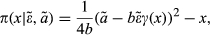
If ρ = 0, then If ρ≠0, then


Proposition 8 suggests that, if there is no correlation between input price and demand, then uncertainty in the latter does not change the value of TI for a firm’s risk management when the firm is risk neutral. Yet by part (a) of the proposition, a strongly risk‐averse firm (λ >
If demand and input–price uncertainties are correlated, then even a risk‐neutral firm may exhibit differential valuations of TI investment. In particular: by Proposition 8(b), if that correlation is positive (resp. negative) then a risk‐neutral firm becomes more (resp. less) interested in TI as demand uncertainty increases. This dynamic follows because demand uncertainty compensates for some of the option value lost owing to the profit function’s reduced curvature. So in this case, the flexible firm views TI’s mean‐reducing effects more favorably and is less concerned about its convexity–reducing effects.
The numerical results graphed in Figure 5 expand this proposition for cases in which the firm is relatively risk averse. Panel (a) shows that, for a given level of TI investment, higher correlation between demand and input–price uncertainty has the effect of reducing 
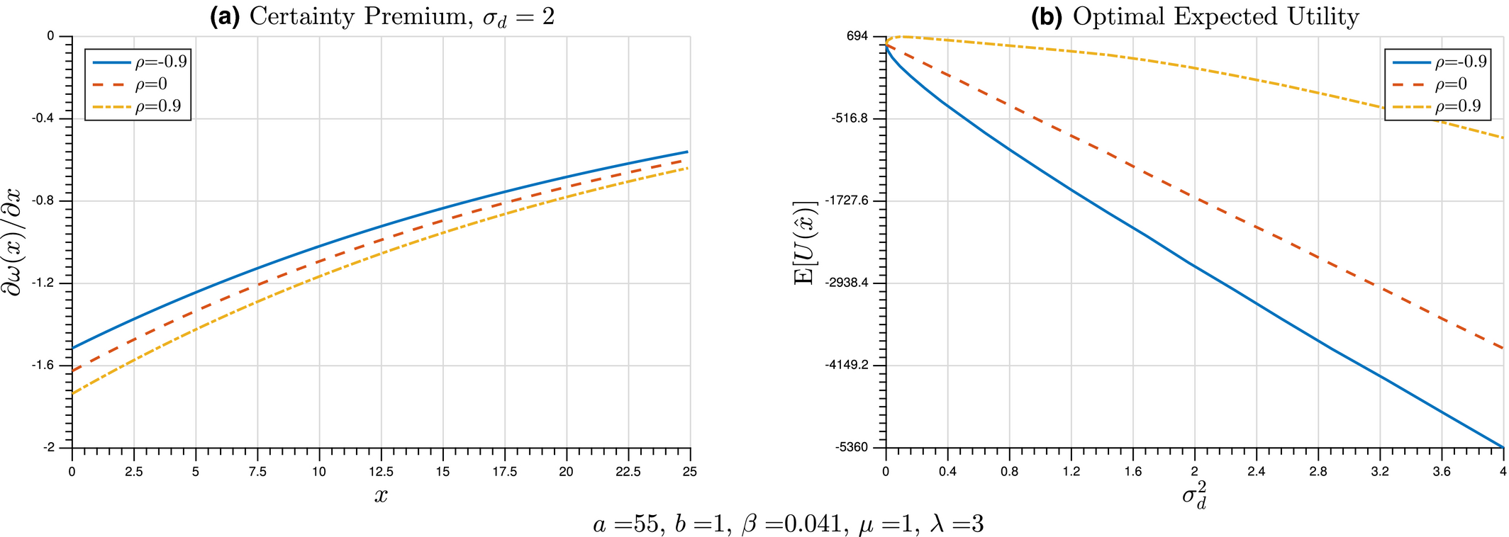
Effects of Demand Uncertainty and of the Correlation between Demand and Input Price on the Certainty Premium and on Optimal Expected Utility [Color figure can be viewed at
Conclusion
This paper’s main objective is to demonstrate formally how TI can be incorporated into a firm’s risk management strategy, especially when financial hedging alternatives are unavailable or too costly. Technology improvement reduces the quantity of inputs needed and, by extension, the variance associated with their cost. However, TI can reduce both the level and variance of input costs, financial hedging typically mitigates only the volatility of those costs.
To characterize firms’ optimal decisions to adopt TI, we develop a theoretical model that enriches our understanding of their attitudes toward input‐price uncertainty. We then use this model to compare TI and FH in contexts where firms can benefit (or do not benefit) from increased volatility in the price of production inputs. This model suggests that the certainty premium is affected by two main factors: the profit function’s structure (i.e., the extent of its convexity or concavity); and the risk attitude effect, which is the product of the firm’s risk aversion and the quantity of inputs used. These two factors drive the changes in a firm’s certainty premium as a function of its investment in TI.
For both the monopoly and competition cases, we show that a firm’s input certainty premium is affected by TI directly and also indirectly (i.e., through the optimal hedging position). These effects can either increase or reduce the value derived from investing in technology improvement, which explains why the optimal level of such investment varies in response to changes in input–price uncertainty. Table 2 summarizes these results.
Interaction between Industry and Firm Type (RA↑, high risk aversion; RA↓, low risk aversion)
Notes: The inequality ω(x) > 0 (resp., ω(x) < 0) means that the effect of uncertainty’s option value on the profit structure is less (resp., greater) than the effect of the firm’s risk attitude (cf. Equation 6). The inequality 

Absent financial hedging, if risk aversion is low then the firm will reduce its TI investment in response to increased price uncertainty; the reason is that investing in technology improvement reduces the option value associated with being exposed to input–price uncertainty. At the same time, this setting results in less risk exposure if firms do engage in financial hedging. Comparing TI and FH from the risk management perspective, we demonstrate that hedging results in a lower certainty premium; that is, the option value resulting from exposure to input‐price uncertainty is higher with FH than with TI. This difference in the risk management value of these strategies increases with the level of uncertainty. It follows that, even though the cost reduction benefits of TI might result in higher expected utility under low uncertainty, the risk reduction benefits of FH under high uncertainty might exceed those due to TI.
Our analysis also answers the question of whether a firm is better off when adopting both strategies. From the risk management perspective, we observe that TI, in isolation, can lower the firm’s certainty premium by reducing the input quantity used. Yet because optimal hedging can eliminate the effect of input quantity used, FH (if available) is always a substitute for TI. From the standpoint of total expected utility, our analysis delivers a more nuanced result: the two strategies are always substitutes in flexible settings, but they are substitutes in committed settings only when risk aversion is low. So for a firm that has pricing flexibility yet is extremely averse to risk, it would in fact be preferable to adopt both strategies.
Duopoly competition adds an instructive dimension to our analysis of the certainty premium. In a duopoly, the flexibly pricing firm’s profit is not always convex with respect to the input price. We show that there is a level of TI investment at which the profit could be either convex or concave, resulting in a (respectively) negative or positive effect on the certainty premium. The threshold at which TI affects the certainty premium depends on the expected input costs—a relation that explains why TI investment decreases (resp. increases) with uncertainty when the mean of input cost is low (resp. high). In the flexible setting, we again observe that TI and FH are substitutes. Yet in the committed duopoly setting we show that, although the profit curve’s convexity has no effect on the certainty premium (
We remark that TI investments often have direct implications also for the “sustainability” of firms’ operations (although this aspect is not incorporated into our model). The higher is TI, the lower will be the consumption rate of variable inputs (e.g., fossil fuels)—in line with the core promises of a sustainable supply chain. It is worth noting that our results reveal another explanation for why some firms are disinclined to invest in sustainable technologies: doing so would reduce their (potentially desirable) exposure to input–price risk. Thus our model predicts that, ceteris paribus, investment in such sustainability initiatives as energy efficiency is higher for: industries with less flexibility in pricing; private firms (which tend to be more risk averse); firms in industries that lack markets for forward contracts of input commodities; and industries for which production efficiency across different plants is relatively more homogeneous (resulting in a less convex profit function). In short, if similar technologies are used by an industry’s firms then they will be more willing to invest in measures that promote sustainability. That said, the net environmental and sustainability effect of a firm’s TI depends crucially on the “footprint” of the input commodity (e.g., jet fuel) and the particular technology used to improve efficiency (e.g., manufacturing solar panels with rare earth materials). A full life‐cycle analysis is required to quantify the overall effect of a firm’s risk reduction strategies on its environmental footprint.
Our analysis can be extended in several directions. First, we assume that investment in TI is a one‐time occurrence in the model’s initial period (Stage 1). Real‐world firms can, of course, engage in multiple rounds of TI investment; that option is being explored and formalized in another study by the authors. Second, the connection between FH and TI is more salient when the risk of bankruptcy is taken into account. More specifically, a firm that uses external funding to invest in TI might need to hedge against high input prices in order to guarantee its debt service on external funding and to avoid bankruptcy. Although our model can be viewed as incorporating bankruptcy risk into the firm’s overall level of risk aversion, one could—by explicitly incorporating external funding and the risk of bankruptcy—further clarify the mechanisms through which input–price uncertainty affects TI investment. Third, this study considers the two extreme cases of full flexibility and full commitment. However, some industries (e.g., shipping) exhibit partial flexibility in adjusting their output prices to reflect input costs. This intermediate variation is an approach that merits further analysis. Fourth, yet another research question worth pursuing is how TI investment affects input commodity prices. If the firm has a large market share, then its investment in TI significantly affects the demand and hence the price of an input commodity. That dynamic could alter the investment decision of such firms, and it might also encourage non‐investing firms to free‐ride on the efforts of investing firms—a phenomenon known as the “green paradox.”
Finally, we solve a model in which the downside and upside risks are symmetric. However, TI can be especially useful in the case of asymmetric upside and downside price risks. A TI project will disappoint its investors ex post if the realized input price is low, since in that case the realized return on TI investment is also low. Yet if the firm faces large upward but small downward price swings, then TI becomes more attractive because it yields a larger expected value. No financial contract (i.e., if it is fairly priced) can provide such an asymmetric return because its price already incorporates the distribution of payoffs.
Footnotes
A. Glossary of Notation
B. Model Calibration and Data
C. Proofs
1
2
3
4
There are many cases in which investment in TI is beneficial even when risk reduction is not a consideration. Apart from the average‐price effect, other benefits include operational robustness (stemming from reduced reliance on the input), environmental sustainability, and the possibility of increased market share due to marginal cost reductions. Such benefits may justify the widespread adoption of TI projects by different firms. We take such potential advantages as given and ask whether TI can, in addition, yield benefits related to risk reduction.
5
A forward market is a fair market when forward prices are equal to the expected value of the realized spot prices.
7
Our model focuses on intermediary commodities (e.g., energy, water) that are not directly consumed by the end customer. Other examples of production inputs that the final consumer does not value directly include the jet fuel for an airline, the gas for a power plant, the electricity for a smelter, and metals for a wind turbine producer. Customers are interested in the end product (e.g., travel services, electricity produced) rather than the inputs used to produce those services or goods. Hence we do not address technology changes that replace resources with more economical commodities.
8
In our model, we capture the uncertainty associated with the outcome of the project by focusing on the financial outcome and allowing the dollar value of savings to be stochastic while abstracting from cases where the TI project may not produce the desired physical results. While being beyond the scope of this study, we believe capturing such technology uncertainty would not change the central insights of this study.
9
The airline, construction, and agriculture production industries all feature committed production plans. Hence firms in these sectors must decide on a production plan prior to observing actual input costs—for example, labor and (respectively) jet fuel, cement, and fertilizer—at the time of production. However, refineries, restaurants, power plants, and food processors are examples of industries that observe their input costs (within a reasonable time frame) and then choose the optimal production quantity.
10
11
Jensen’s inequality is that
12
How uncertainty affects the expected return also defines the riskiness of a firm’s revenue process. The weighted average cost of capital is a function of the firm’s market Beta (i.e., the co‐movement of its stock return and the return on the aggregate market index), and firms that are more risky must pay a higher premium in the equity market in order to raise capital. If TI reduces the firm’s riskiness, then it also reduces the cost of capital for future units of investment and thereby introduces additional incentives to lower risk further. However, our analysis does not incorporate that synergistic effect.
13
An alternative is to use options contracts, which allow for nonlinear risk exposure. For call options, we write
14
We assume that the market for forward contracts is fair in this sense: forward prices are equal to the expected value of the realized spot prices; in other words, there is no basis risk. Such equality is possible provided that there are no major frictions, the intermediary market is competitive, and the market is risk neutral at the aggregate level. This aggregate risk neutrality does not imply that each agent is risk neutral; it simply requires that the total risk aversion of the market’s “long” side be equal to that of its “short” side. We assume that the hedging pressures of these two sides neutralize each other and hence that forward contracts are unbiased.
15
In practice, firms often hedge less than the optimal quantity. One reason is that hedging contracts are not always fair and may involve additional costs. Another is that firms adopt cross‐hedging strategies—that is, taking the opposite position in another commodity with the same or similar price changes. One example is the hedging positions of airlines (described by Carter et al. ![]() ); those positions cover, on average, only 15% of the next year’s (expected) required fuel.
); those positions cover, on average, only 15% of the next year’s (expected) required fuel.
16
Prices in a competitive industry are typically more volatile than the prices set by a monopolist. Competitive markets pass all of a demand or supply shock on to consumers, whereas part of such shocks are absorbed by the monopolist’s profit margin. So even though prices are more volatile in competitive markets, the profit margin of a single firm is more stable.
17
We do not consider the case of one flexible and one committed firm.
18
For additional details see
19
20
21
22
Taylor expansion results in
23
We assume f(x) is well‐behaved which restores its concavity (or convexity) within the feasible domain.