On the Non‐Equivalence of Trade‐ins and Upgrades in the Presence of Framing Effect: Experimental Evidence and Implications for Theory

Abstract

Manufacturers of durable goods often buy back older versions of their products from customers to encourage them to switch to improved versions and to create control over product return streams in their closed‐loop systems. Classical models and conventional wisdom have long ignored that the framing of these buyback schemes, whether through trade‐ins or upgrades, can matter for theory. Using the reference‐point shift mechanism, we provide experimental evidence that the alternative frames are not equivalent and that the framing effect induces customers to change which prices they anchor to as their reference points for the price for their current version. We then use the experimental findings to extend a reference‐dependence version of the classical model of trade‐ins and upgrades and show how the behavioral extension modifies key predictions of the classical model and provides predictions more in line with today's durable goods markets.

Keywords

trade‐in upgrade framing effect reference dependence durable goods

Introduction

A large fraction of purchases of consumer durables is to replace older models. For most consumer electronics, such as computers, digital cameras, and cell phones, replacement purchases account for more than 50% of new products’ total sales (Gordon 2009). For example, more than 80% of potential buyers for a new iPhone series are customers who upgrade from previous iPhone versions (Statista 2014, Statisticbrain 2016). These high rates of replacement purchases, especially for high‐tech consumer electronics, are helped by rapid improvements that have made new product introduction cycles shorter than the useful life of durable goods (Gordon 2009, Ray et al. 2005). For these products, manufacturers rely on replacement purchases to sell new versions of their products (see, e.g., Golson 2016, Kohler 2016). It is now common practice for manufacturers to manage replacement purchases separately from their sales channels for first‐time buyers. In doing so, manufacturers usually engage in price discrimination between replacement and new buyers, typically by buying back older versions of their products or offering price reductions to the replacement buyers (Golson 2016, Ray et al. 2005).¹

Replacement purchases have also become useful mechanisms for durable goods manufacturers to efficiently manage their closed‐loop operations by creating better control over their product return streams. The success of any closed‐loop system depends on the efficiency of its product return stream (Dutta et al. 2016, Li et al. 2011, Tang and Zhou 2012), and replacement purchases, in particular, can help manufacturers manage the quantity, quality, and timing of their product returns (Guide and Wassenhove 2001, Souza 2013).

Trade‐ins and upgrades are two common schemes for replacement purchases. With a trade‐in, replacement buyers are quoted a trade‐in price for their current product when buying its newer version at its regular sales price. With an upgrade, replacement buyers are offered the new version at a discounted price (i.e., an upgrade price) upon giving their current version to the dealer. In standard economic analysis, the two mechanisms are equivalent when the trade‐in value on the old version is equal to the discount value on the upgrade and thus they have often been used interchangeably in the long‐standing literature on trade‐ins and upgrades (see, e.g., Agrawal et al. 2016, Fishman and Rob 2000, Fudenberg and Tirole 1998, Levinthal and Purohit 1989, Li et al. 2011, Rao et al. 2009, Ray et al. 2005, Van Ackere and Reyniers 1993,1995,Zhang and Zhang 2018, Zhao and Jagpal 2009). This equivalence assumption, by ignoring behavioral influences in replacement buyers’ decision‐making, does not let us obtain predictions from the classical models to explain some of the dynamics of today's markets.

There is ample evidence that customers’ decision‐making in replacement purchases is driven mainly by behavioral influences (see Guiltinan 2010 for a review). In particular, the equivalence of trade‐ins and upgrades can no longer be expected to hold once one considers the framing difference between them: Trade‐ins separate the selling transaction of the replacement purchase explicitly, while upgrades embed it in the buying transaction. This framing difference resembles some of the seminal examples of the framing effect provided by Tversky and Kahneman (1981) and Tversky and Kahneman (1986) and is particularly important to study because previous research has shown that, although replacement purchases comprise two simultaneous selling–buying transactions for customers (Okada 2001, Purohit 1995), customers are more sensitive to selling transactions than to buying transactions in replacement purchases (Hoyer et al. 2002, Kim et al. 2011, Purohit 1995, Zhu et al. 2008).

In this paper, therefore, we study the framing effect in trade‐ins and upgrades and postulate that it will result in different evaluations of the selling transaction in a replacement purchase. To approach this framing comparison of trade‐ins and upgrades in a systematic way, we use the reference‐point shift mechanism, which has been established as the proper mechanism for capturing framing effects (see, e.g., Heath et al. 1995, Hossain and List 2012, Lehner 2000). The main logic is that the reference point is the hinge in evaluating any transaction (Tversky and Kahneman 1991) and that two alternative frames would result in different evaluations of the same transaction if and only if they induce different reference points in the transaction (see, for instance, Hossain and List 2012 for reference‐point shifts with reward vs. penalty salary frames). Our main research question is thus whether trade‐ins and upgrades are different in terms of customers’ reference points for the price for their current product. Similar to reference point studies with multiple price anchors (see, e.g., Baucells et al. 2011), through an experimental study, we extract the influential price anchors, among the set of all potential price anchors, on the reference point with both the trade‐in and the upgrade frames. Understanding what influences replacement buyers’ reference points, and how it shifts with the alternative frames, will reveal the leverage that manufacturers can use to manage their customers’ reference points and thus their replacement decisions. Our study is the first to explore the framing difference between trade‐ins and upgrades. Therefore, to provide comprehensive input for future analytical research on trade‐ins and upgrades by durable goods manufacturers under different market settings, we cover all possible market settings in our study in line with the seminal models of trade‐ins and upgrades.

We find that the upgrade frame, by embedding the selling transaction in a net buying transaction, directs customers’ attention toward price anchors relevant to the buying position (i.e., the manufacturer's sales prices), while the trade‐in frame places customers in an explicit selling position and results in anchoring to prices relevant to that position (i.e., the secondary market price). To put it simply, the reference point shifts with the trade‐in and the upgrade frames as a result of anchoring to different prices. We further find that different market settings influence the reference point with a given frame only if they affect the price anchors relevant to the induced position.

By capturing the framing effect in trade‐ins and upgrades through reference‐point shifts, our experimental findings are of direct applicability to developing behavioral models of trade‐ins and upgrades through incorporating reference dependence in analytical models (as an established method of developing behavioral models; Ko˝szegi and Rabin 2006). To illustrate an implication of our findings, we develop a reference‐dependence version of the classical model of trade‐ins and upgrades by Fudenberg and Tirole (1998). Our model extension revisits their predictions that under a high innovation level in the new version, the manufacturer will not continue production and sale of the original version alongside the new version and that the manufacturer is better off with trade‐ins than upgrades. This prediction is, of course, at odds with the numerous instances we see in today's markets where manufacturers have overlapping production even under a high innovation level in the new version. For instance, Apple continued production of the iPhone 4s until September 2014, a full year after the iPhone 5s and 5c were introduced to the market. Similarly, the iPhone 5s remained available until March 2016, over a year after the iPhone 6 and 6 Plus were introduced.² These dynamics exist even though, driven by Apple's very large R&D investments (Appleinsider 2016), the new iPhone series is produced with similar production costs yet obtaining high consumer valuations and sales prices (Time 2014, 2016), which fall under the high innovative category by Fudenberg and Tirole (1998). While common explanations, e.g., market segmentation and technology adoption, do not apply here, our reference‐dependence extension provides another explanation that manufacturer's objective in continuing production of older versions is to manage the upgraders’ reference points through the sales price of the older version. That is, the manufacturer continues producing the older version and drops its price significantly to reduce the upgraders’ expectations as to the price for their current version.

The remainder of the study is organized as follows: section 2 covers the related literature and builds the hypotheses; section 3 describes the experimental study; section 4 presents and discusses the experimental results; section 5 provides a comparison between predictions of the classical model and those of the reference‐dependence model; and finally, section 6 concludes the paper.

Hypotheses

Since its introduction by Tversky and Kahneman (1981), the framing effect has been observed in many different contexts, and in both laboratory and field experiments,³ from pricing contracts (Ho and Zhang 2008, Lim and Ho 2007) to financial investments (Cheng and Chiou 2008, Kumar and Lim 2008) health communications (Gallagher and Updegraff 2012), and work performance (Hannan et al. 2005, Hossain and List 2012, Luft 1994). It has been shown that even experimental economists are prone to the framing effect (Gächter et al. 2009). Related to our context, Monga and Zhu (2005) and Yang et al. (2013) found that buyers and sellers respond differently to the same frame, and Simonson and Drolet (2004) showed that different anchors have different effects on buyers’ and sellers’ decisions. Here, reasoning that trade‐ins and upgrades differ in framing the selling transaction for replacement buyers, we postulate that these alternative frames result in customers anchoring to different prices as their reference points for the price for their current product. Precisely, trade‐ins separate the selling transaction for customers and put them in a selling position, while upgrades embed that selling transaction in the buying transaction and thus keep them in a buying position. Therefore, we expect that, driven by the induced position, with a trade‐in frame, customers would anchor to prices relevant to the selling position, while with an upgrade frame, they would anchor to prices relevant to the buying position. We present this prediction in the following hypothesis:

Hypothesis 1

With a trade‐in (respectively, an upgrade), customers anchor to prices relevant to the selling (respectively, buying) position as their reference points for the price for their current version.

To further narrow down this hypothesis to whether and how different market settings would change customers’ reference points with the two frames, we fit our problem setting with that of the classical model of trade‐ins and upgrades by Fudenberg and Tirole (1998), which has been used quite often in the literature of replacement purchases. A monopolist (hereafter, the manufacturer, she) produces two successive versions of a durable product over two periods. In period one, only the original version is produced and sold. In period two, the manufacturer introduces the new version with a high or low innovation and offers trade‐ins or upgrades to her former customers (i.e., replacement buyers) in addition to selling to new buyers. Upon introducing the new version in period two, the manufacturer may or may not decide to continue production and sale of the original version. This setting creates four potential price anchors for replacement buyers at the replacement purchase point: the price they paid in period one to purchase the original version; its current sales price; its secondary market price; and the new version's sales price.⁴ The secondary market price is the only price anchor relevant to the selling position, while the other three, coming from the manufacturer's sales channel, are relevant to the buying position, among which the new version's price is the most relevant one.

With this framework, changes in three dimensions can impact the dynamics of the market setting: the innovation level in the new version (which determines whether or not the two successive versions, and their prices, are comparable to each other); the existence or absence of an external secondary market (which determines the existence or absence of a potential price anchor for replacement buyers); and whether the manufacturer continues production and sale of the original version alongside the new version (which determines the existence or absence of another potential price anchor). The latter two change the general setting of the market as they add or remove a potential price anchor to or from the market. The first dimension, on the other hand, alters an existing market setting by shifting an existing price anchor along a given dimension. We next explore the effect of change in each dimension on the reference point with each frame. Table 1 illustrates these three dimensions and summarizes our hypotheses for both the trade‐in and upgrade frames.

Table 1

Hypotheses

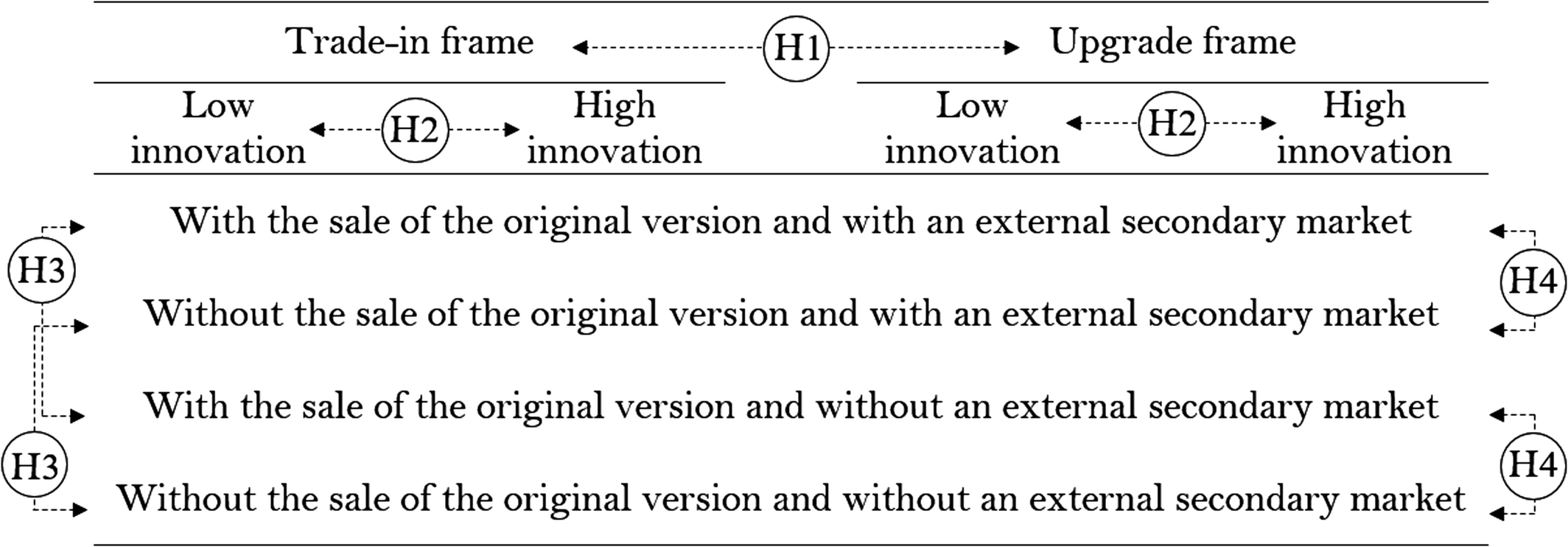
Exploring the effect of the first dimension—that is, the new version's innovation level—on customers’ reference points directly relates our study to previous research on manufacturers’ new product introductions. Most of the work in this area is in line with our setting, that is, a two‐period model with discrete product quality/innovation levels (see, e.g., Kornish 2001, Waldman 1996). The need for studying novel directions in new product introductions was first highlighted by Waldman (2003), and there have been extensions since then. Related to our study, Okada (2006) found a significant difference in replacement buyers’ interest in a new product, relative to new buyers’ interest, between when the new product was similar to their current product and when it was dissimilar to it. This relative difference comes from a change in how replacement buyers close their mental accounts for their current product (Thaler 1980, 1985), influenced by the perceived (dis)similarity of the new product to their current product, which roots in the general theory of similarity by Tversky (1977). Here, we relate this (closing the mental account for the current version) to a shift in replacement buyers’ reference points for a price for their current version driven by the new version's innovation level and its price as the representative of (dis)similarity to the current version. The new version's price is the most relevant price anchor to the buying position and thus to the upgrade frame. Hence, the new version's innovation level would determine whether or not this price anchor could be a comparable point of reference for customers with the upgrade frame. When the new version is a high innovation and thus cannot provide a comparable point of reference, customers may refer to another price anchor relevant to the buying position (in this case, the current sales price of their current version, which is the next most relatable price anchor from the buying position). Therefore, we expect that the new version's innovation level will shift customers’ reference points with the upgrade frame. On the other hand, as it does not influence the price anchor relevant to the selling position, it will not change the reference point with the trade‐in frame. The following hypothesis summarizes:

Hypothesis 2

The innovation level of the new version shifts customers’ reference points with the upgrade frame, while it will not change the reference point with the trade‐in frame.

The second dimension—that is, the existence or absence of an external secondary market—is usually out of the manufacturer's direct control, but can be manipulated by indirect strategies (see Hendel and Lizzeri 1999 for a good discussion on this). Studying the costs and benefits for manufacturers in doing so is beyond the scope of this study(on this topic, see Benjamin and Kormendi 1974, Chen et al. 2013, Levinthal and Purohit 1989, Liebowitz 1985, Oraiopoulos et al. 2012, Rust 1986). What we explore here is how the existence or absence of an external secondary market will influence customers’ reference points with the two replacement purchase frames. From what we discussed earlier, we expect that it will not shift customers’ reference points with the upgrade frame because it does not change the price anchors relevant to the buying position. However, it will change the reference point with the trade‐in frame, wherein the secondary market price is the only price anchor relevant to customers’ selling position. This leads to the following hypothesis:

Hypothesis 3

The existence or absence of an external secondary market will shift customers’ reference points with the trade‐in frame, while it will not change the reference point with the upgrade frame.

The third dimension—that is, whether the manufacturer continues production and sale of the original version after introducing the new version—is also a dimension influencing the price anchors relevant to the buying position because it determines the existence or absence of a price anchor in the manufacturer's sales channel. Changes in this dimension are particularly determinant of customers’ reference points with the upgrade frame under a high innovation level in the new version, wherein the new version's price is not a comparable point of reference, and customers are likely to anchor to the current sales price of their version as their reference point. In this case, the manufacturer's not continuing production and sale of the original version eliminates this possible reference point for customers, and the only remaining price anchor relevant to the buying position becomes the original purchase price coming from period one. Hence, changes in this dimension will influence the reference‐point shift with the upgrade frame that Hypothesis 2 predicted. When the new version is a low innovation, on the other hand, this will not influence the prediction of Hypothesis 2 because the new version's price is still present and the most relevant price anchor to the buying position. In addition, similar to our predictions in previous hypotheses, we expect that a change in this dimension will not shift the reference point with the trade‐in frame because it does not influence the price anchors relevant to the buying position. We present these expectations in the following hypothesis:

Hypothesis 4

The manufacturer's decision not to sell the original version at the replacement purchase point shifts customers’ reference points with the upgrade frame when the new version is a high innovation, while it will not change the reference point with the trade‐in frame.

Experimental Study

Design

To increase the external validity of our results, we match the experimental setting with a real‐life situation: trading in or upgrading an electronic tablet. In addition, in order to capture the time point of decision‐making in replacement purchases, we need to use an imaginary situation: currently using a tablet and thinking about replacing it with its newer version. This is a common approach in previous experimental studies on replacement purchases (see, e.g., Kim et al. 2011, Purohit 1995, Srivastava and Chakravarti 2011, Zhu et al. 2008) and has been used in other decision‐making problems, as well (see, e.g., Baucells et al. 2011 for reference points in selling stocks, and Hardisty and Pfeffer 2016 for people's choices between present and future payoffs). There is also ample evidence that respondents’ decisions in imaginary and real‐life situations do not differ significantly (see, e.g., Carmon and Ariely 2000 and references therein).

Because we study reference points, we are looking for the price that would make participants indifferent to making the replacement purchase transaction. Our approach is similar to that of Baucells et al. (2011) in their extraction of the reference point in selling a stock, where they asked participants for the price that would make them “neither happy nor unhappy about the sale.” As Baucells et al. (2011) noted, “Because of the pure psychological nature of the reference point, no ‘incentive‐compatible’ variable payment could be used” in these settings. Yet, because our experimental situation concerns a decision about a physical product, to make sure about eliminating potential attachment effects (and the price inflation they may induce), we apply the approach successfully implemented by Purohit (1995), Zhu et al. (2008), and Srivastava and Chakravarti (2011) and define the experimental situation for a third party. That is, we describe a third‐party situation and ask participants about the price for that person's current product that would make him “indifferent” about the replacement purchase.

We start with the experimental design for the trade‐in frame. To identify the reference‐point value in the selling transaction, we first need to keep the buying transaction's utility (i.e., the difference between participants’ willingness to pay for the new version and its consumption utility) zero. Failure to do so would interfere with the procedure of reference‐point elicitation. Hence, we present the participants with two purchase options that our third‐party, “Jack,” is offered: a pure purchase and a trade‐in. With this setting, the price that participants think would make Jack indifferent between the two options is the price they think would bring him zero utility in selling his product, that is, the reference‐point value in the selling transaction. The experimental task is described to participants as follows (the prices shown here are just examples):

Jack has a fully functioning Tablet 4.2 (a brief description is provided below), which he had purchased for $190. A Tablet 4.2 is currently sold at $165. The average price of a used Tablet 4.2 of the same condition as Jack's is $60.

[Tablets 4.2 and 5.0 specifications were shown here; see Appendix A]

Jack is thinking about buying a Tablet 5.0, and there are two purchase options available to him:

Option (1) Store A sells the Tablet 5.0 for $270.

Option (2) The same store has a trade‐in program. That is, the store will pay Jack cash for his current tablet if he gives it to that store when purchasing the Tablet 5.0 at the same price as in Option 1 ($270).

How much cash do you think Jack should receive to be indifferent between these two options?

To study the framing effect, we change the experimental question to the upgrade frame as follows:

Option (1) Store A sells the Tablet 5.0 for $270.

Option (2) The same store has an upgrade program. That is, the store will sell Jack the Tablet 5.0 at a lower price (p) if he gives his current tablet to that store.

At what price p do you think Jack would be indifferent between these two options?

The reference‐point value in the selling transaction here is calculated by subtracting the indicated lower price (p) from the new version's price.

The objective of our experiment is to extract which of the price anchors participants would refer to (as their reference points) when deciding their indicated values under different market settings. Having enough data points for each market setting, we can do so by investigating changes in which of the price anchor have the highest influence on the change in the reference‐point value (see section 4). With the problem setting we study, the original version's purchase price and the new version's price are potential price anchors always available regardless of the market setting. In contrast, the current sales price of the original version and the secondary market price may or may not exist (depending on the manufacturer's decision whether to continue production and sale of the original version at the replacement purchase point, and the existence or absence of the external secondary market, respectively). These create four possible settings with different sets of potentially influential price anchors (as summarized in Table 1). The additional dimension—that is, the discrete innovation level of the new version (low or high)—creates two versions of each of these four settings. For them, we consider two new versions with distinct (low and high) innovation levels and sales prices: Tablets 5.0 and 5.2, with the improved features and the sales price relatively high for the latter. Therefore, we have eight virtual market settings in total. We adjust the experimental question for each market setting by removing the part about the current sale of the original version, removing the part about the secondary market, and offering Tablets 5.0 or 5.2 as the new version.

Procedure

We recruited 1,195 participants (45.2% female; M_age = 36.46, SD = 11.62) via Amazon Mechanical Turk (AMT) and paid a flat fee ($0.60) for their participation. Participation was restricted by location (the U.S. only) and acceptance rate (above 97% with more than 5000 hits). The main advantage to using AMT is to access at reasonable cost a large population of average people and thereby to obtain responses likely to be closer to typical market behavior. AMT has become a popular avenue for subject recruitment in experimental studies, and several studies have endorsed AMT from different aspects as a reliable source of experimental data (see, e.g., Hauser and Schwarz 2016, Lee et al. 2018 and references therein). The majority of our sample had education beyond high school: 31.2% had some college credit, while another 45.2% reported having earned a Bachelor's degree. The average annual income was in the range $25,000–$49,999.

After agreeing to participate in the study, participants were referred to an external platform (Qualtrics) for the experimental task. After answering some demographic questions, participants were randomly assigned to either the trade‐in or the upgrade frame under one of the four market settings (as shown in Table 1). Each participant answered two questions in random order, one for the low innovation level and one for the high innovation level, with different price sets.⁵ In indicating their responses, each participant saw a different set of prices randomly drawn from the predefined intervals given in Table 2. The price intervals were chosen in a way that all possible ratios between the four potential price anchors are realistic, based on real market products and prices. For instance, the average secondary market price is kept between 14% and 53% of the original purchase price and between 16% and 67% of the current sales price. Furthermore, the price range for the new version under a high innovation is set to create relative prices high enough to match the high innovation nature of the new version. In contrast, the price range under the low innovation makes sure of having prices close enough to that of the original version to resemble a low innovation level in the new version.

Table 2

Price Intervals (in dollars)

Price	Interval*
Original purchase price	[170–230]
Average secondary marlet price	Original purchase price − [110–145]
Current sales price of the original version	Original purchase price − [15–50]
New version's price under a low innovation level	Original purchase price + [50–105]
New version's price under a high innovation level	Original purchase price + [210–265]

*All random numbers are generated in increments of 5.

To help with the regressions, we run for each experimental group (see section 4), while keeping the assignment process random, we assign more participants to the groups for market settings with more potentially influential price anchors (e.g., more participants in the experimental group representing the first setting in Table 1 than in the one representing the fourth setting). This helps ensure that we have enough data points for the regressions given the number of independent variables in each experimental group. Table 3 shows the total number of responses in each experimental group (we have relatively more data in the first market setting in the interest of performing some robustness checks; see Appendix C).

Table 3

Total Number of Responses in Each Experimental Group

Setting	Trade‐in frame		Upgrade frame
Setting	Low innovation	High innovation	Low innovation	High innovation
With the sale of the original version	240	240	240	240
With an external secondary market
Without the sale of the original version	133	133	129	129
With an external secondary market
With the sale of the original version	131	131	131	131
Without an external secondary market
Without the sale of the original version	96	96	95	95
Without an external secondary market

We ensure the reliability of responses by applying filtering criteria, including an attention‐check question, filtering obviously false data and ruling out outlier responses using Tukey's outlier criterion in each experimental group, that is, responses below Q ₁ − 1.5 × [Q ₃ − Q ₁] and above Q ₃ + 1.5 × [Q ₃ − Q ₁], with Q ₁ and Q ₃ being the first and the third quantiles in the group, respectively (Seo 2006). However, unless we have a strong reason to filter false data, such as participants’ misunderstanding or responses of 0 because participants were not able to enter a valid number, we leave the data cleaning to the outlier criterion (for instance, we do not exclude any data because of the participant's response time). Our attention‐check question at the end of the experimental task (available in Appendix A) is designed to ensure that participants read and paid enough attention to the described situation (see Abbey and Meloy 2017, who discuss various attention‐check questions commonly used in experimental studies). Together with the attention‐check failures, the final data loss is under 19.8 percent.⁶ Inclusion of the filtered data in the analysis did not change the final results, nor did it influence the significance levels, and only changed some of the p‐values (see Abbey and Meloy 2017 for a thorough discussion on inclusion and exclusion of attention‐check failures in experimental analyses).

Similar to reference‐point elicitation by Baucells et al. (2011), followed by the main experimental task, participants were also asked directly how important, on a 7‐point Likert scale, each of the prices were for them in arriving at their response. Answers to this question were mainly confirmatory with no new insights, and hence we do not include them here. We also asked participants about the clarity of the explained situations, on a 1–5 scale (5 being “very clear”), and the average score was 4.2.

Experimental Results

Preface Analysis

We start analyzing the experimental results with a general analysis on the effect of the alternative frames on participants’ reference points. We use a mixed‐model analysis to investigate whether the alternative frames make a statistically significant difference in participants’ reference points under different market settings. Based on Table 1, we have a 2 × 4 × 2 design in this analysis, capturing the two frames, four market settings, and two innovation levels, respectively. This is a mixed‐model analysis with the first two factors being between‐subject factors and the third one being a within‐subject factor.

Table 4 shows the result of this analysis. As the first row shows, there is a clear framing effect on participants’ reference points. The second row uncovers that the two alternative frames also have different effects under different market settings. Finally, the third row shows that the innovation level (i.e., low and high) makes a statistically significant difference on the framing effect under different market settings. The last row checks whether the order in which participants see the low innovation and high innovation cases influences the results.⁷ As seen, there is no such effect from the order—this is in agreement with the result of the robustness check we perform on using the same participants for both innovation levels (see Appendix C).

Table 4

Results of the Mixed‐Model Analysis

Term	Number of levels	F	Significance
Frame	2	1901.74	<0.001
Frame × Market	8	12.23	<0.001
Frame × Market × Innovation	16	9.78	<0.001
Frame × Market × Innovation × order	32	1.06	>0.385

Framing Effect and Reference‐Point Shift

Having established that there is a framing effect with the trade‐in and upgrade frames, we now aim to extract reference points with the two frames under different market settings to answer our main question on the reference‐point shift between the two frames. To do so, referring to the regression‐based methodology of Baucells et al. (2011) in extracting the price anchors with statistically significant influence on the reference point, we use regression models with all the potentially influential price anchors as independent variables and the reference point as a dependent variable. We use Hierarchical Regression (HR), which among a set of independent variables finds the ones with significant influence on the dependent variable, to identify the price anchor(s) with the highest statistically significant influence on the reference point. Regression models for the trade‐in and upgrade frames are as follows, respectively:

r e f_{i}^{T} = α + α_{o} O p p_{i} + α_{s} S e c_{i} + α_{c} C u r r_{i} + α_{n} N e w_{i} + ε_{i}

(1)

\begin{matrix} r e f_{j}^{U} = & N e w_{j} - p_{j} = β + β_{o} O p p_{j} + β_{s} S e c_{j} \\ + β_{c} C u r r_{j} + β_{n} N e w_{j} + ε_{j} \end{matrix}

(2)

The

r e f_{i}^{T}

and

r e f_{j}^{U}

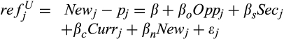
are the extracted reference‐point values from participants i and j under the trade‐in and upgrade frames, respectively. The independent variables Opp, Sec, Curr, and New indicate the original purchase price, the average secondary market price, the current sales price of the original version, and the new version's price, respectively. Because of the nature of the dependent variable, the intercept will not have a meaningful interpretation (that is, when all prices are zero in the market, that is, everything is free, customers’ reference points are zero, as well) (Baucells et al. 2011). It is important, however, when the intercept is the only significant part of the regression's outcome, which would mean none of the anchors explains the reference point properly. Thus, we start running Hierarchical Regressions with an intercept, and if only the intercept is significant, we conclude that no anchor explains the reference point. If the intercept is significant along with one or more prices, we take those price(s) to be the influential one(s). If the intercept is not significant, in line with the logic of Hierarchical Regression, we remove it from the regression model and take the outcome price(s) to be the influential one(s). Finally, if the regression yields more than one significant price, we statistically compare their coefficients (using a z‐test) to find the most influential price anchor. As the comparison will be between coefficients of different price anchors, we will use standardized coefficients to take into account the standard deviations, as well.

In running the HR for each group, only the independent variables corresponding to the potential anchors in that group (based on Table 1) are kept in the regression model. If two groups turn out to have different influential anchors, we conclude that they differ in terms of the reference point. If, on the other hand, two or more groups have the same influential anchor(s), we statistically compare the influential anchors’ coefficients across them to conclude their difference or equality in terms of the reference point. In the between‐group comparisons, we limit the regressions only to the extracted most influential anchor(s) because only those anchors would appear in the manufacturer's reference‐dependence model. We use a z‐test to statistically compare coefficients’ magnitudes for the same price anchor across different regressions (see Clogg et al. 1995).

Reference Points with Trade‐ins and Upgrades

If framing matters, all else being the same, we should see different reference points with the trade‐in and upgrade frames. Table 5 shows that this is, in fact, the case. With the upgrade frame (see columns (3) and (4)), participants anchor to a price relevant to the buying position as their reference point. This price could be the new version's price, the current sales price of their version, or its original purchase price, depending on the market setting. On the other hand, with the trade‐in frame (see columns (1) and (2)), as long as there is an external secondary market, participants anchor to the secondary market price (i.e., the only price anchor relevant to the selling position) as their reference point. These provide supporting evidence for Hypothesis 1.

Table 5

Influential Anchors on the Reference Point with the Alternative Frames in Different Market Settings

Setting	Trade‐in frame		Upgrade frame
	Low innovation	High innovation	Low innovation	High innovation
	(1)	(2)	(3)	(4)
With the sale of the original version	Sec	Sec	New	Curr
With an external secondary market	(<0:001)	(<0:001)	(<0:001)	(<0:001)
	0.90	0.95	0.27	0.60
Without the sale of the original version	Sec	Sec	New	Opp
With an external secondary market	(<0:001)	(<0:001)	(<0:001)	(<0:001)
	0.94	1.04	0.32	0.49
With the sale of the original version	Curr	Curr	New	Curr
Without an external secondary market	(<0:001)	(<0:001)	(<0:001)	(<0:001)
	0.61	0.66	0.38	0.91
Without the sale of the original version	const	const	New	Opp
Without an external secondary market	(<0:001)	(<0:001)	(<0:001)	(<0:001)
	91.48	106.54	0.38	0.74

Notes

Parentheses contain p‐values. In all cells, HR yields only the indicated price with a significant influence on the reference point (full regression models are available in Appendix B). Numbers in the third row are the coefficients used in between‐group comparisons as explained in the text.

The Role of the Innovation Level

Comparing column (4) to column (3) of Table 5 shows that, as predicted in Hypothesis 2, the new version's innovation level shifts the reference point with the upgrade frame (from New to Curr or Opp, depending on the manufacturer's decision whether to continue production and sale of the original version), while it does not influence the reference point with the trade‐in frame (compare column (2) to column (1)). The new version's price is the most relevant price anchor to the buying position, so participants anchor to that as their reference point. This is only the case, however, when the new version is a low innovation and its features and price can provide a comparable point of reference for participants’ current version. When the new version is a high innovation and its features and price are far from the current version, participants anchor to the current sales price of their version as the next most relevant price anchor to the buying position. When this price is not available (due to the manufacturer not continuing production and sale of the original version), participants anchor to the next price anchor relevant to the buying position, that is, the original purchase price of their version.

The Role of the Secondary Market

As seen in Table 5, the above shifts in the reference point with the upgrade frame are irrespective of the existence or absence of the external secondary market. Comparing the top two rows to the bottom two rows, which only differ in the existence of the secondary market price, we see the exact same pattern in the reference‐point shift with the upgrade frame (i.e., a shift from New to Curr or Opp, only depending on the manufacturer's decision whether to continue production and sale of the original version). On the other hand, the existence or absence of the external secondary market fundamentally changes the reference point with the trade‐in frame (compare the top two rows to the bottom two rows for the trade‐in frame). As long as there is an external secondary market, participants anchor to the secondary market price. However, when there is no external secondary market, and thus the only price anchor relevant to the selling position is not available, participants anchor to the current price of their product, which to some extent, can provide them with an estimate of what their current version could sell for. When this price is also removed (due to the manufacturer not continuing production and sale of the original version), none of the remaining prices provides a price anchor directly or indirectly relevant to the selling position. Hence, we do not see a clear anchoring to any of the remaining prices in this case. These provide supporting evidence for Hypothesis 3.

The Role of the Overlapping Production

Finally, Table 5 also shows supporting evidence for Hypothesis 4. Comparing the second row to the first row (and similarly, the fourth row to the third row), we see that with the upgrade frame under a high innovation level in the new version, the manufacturer not continuing production and sale of the original version shifts participants’ reference points from the current sales price of their version to its original purchase price. As predicted, no shift happens in the reference point when the new version is a low innovation because participants always anchor to the new version's price. Similarly, with the trade‐in frame, as long as there is an external secondary market, and thus participants anchor to the secondary market price as their reference point, the manufacturer's decision not to continue production and sale of the original version does not influence the reference point (compare the second row to the first row for the trade‐in frame). With the trade‐in frame, it only matters in the market settings without an external secondary market (see the bottom two rows), wherein participants use the current sales price of their version as an approximation of what their product would sell for. In these market settings, the manufacturer not continuing production and sale of the original version eliminates this price anchor and results in no clear anchoring to any of the remaining prices because none of them is directly or indirectly relevant to the selling position.

General Discussion

The experimental results show that the effects of the innovation level, the secondary market, and the overlapping production on replacement buyers’ reference points depend on the frame of the replacement purchase offer. They may shift the reference point with one frame, while having no effect with the other. We highlight a couple of points on each.

On the role of the new version's innovation level, the most notable is that while shifting the reference point with the upgrade frame, it does not change the reference point with the trade‐in frame. Moreover, we find no statistically significant difference between the coefficients’ magnitudes in column‐wise comparisons of the coefficients (all p > 0.080 in two‐tailed z‐tests for columns (1) and (2) in Table 5).⁸ It is also important to note how the innovation level shifts the reference point with the upgrade frame. When the new version is a low innovation, the manufacturer is able to keep the replacement buyers’ decisions tied only to the new version's price and has thus a single control variable to influence both new buyers’ and replacement buyers’ decisions. With a high innovation level in the new version, in contrast, the manufacturer has an advantage of controlling replacement buyers’ decisions by prices other than the new version's price, which, depending on the circumstances, can provide more flexibility for the manufacturer in adjusting her sales prices.

On the role on the secondary market, the most notable is its exact opposite role to that of the innovation level: Eliminating the secondary market does not shift the reference point with the upgrade frame, while it changes the reference point with the trade‐in frame. It is also worth noting that although the secondary market price does not shift the reference point with the upgrade frame, its elimination seems to increase the reference‐point value by increasing the anchoring coefficient (0.27 vs. 0.38, 0.60 vs. 0.91, etc., as seen in columns (3) and (4) in Table 5). The secondary market price is the smallest number that participants observe in the experiment, and hence its presence or absence may impact the range of values reported by the participants after anchoring to the chosen reference point. To examine this secondary role of the secondary market price more carefully, we define a dummy variable for the existence or absence of the secondary market and run the following regressions over the pooled data for when the current sales price of the original version is the reference point (in Appendix C, we repeat the same analysis for when the original purchase price is the reference point and for when the new version's price is the reference point and obtain similar results):

r e f_{j}^{U} = β_{c} C u r r_{j} + β_{d} d u m m y_S e c_{j} + β_{cd} C u r r \times d u m m y_S e c_{j} + ε_{j}

(3)

The dummy variable dummy_Sec _j equals 1 if participant j had the secondary market price in her/his experimental task and is 0 otherwise. The Curr × dummy_Sec _j, in addition, captures any variable effect driven by the presence of the secondary market price. Table 6 shows the outcome of this regression. We see a negative, but statistically insignificant, fixed effect from the presence of the secondary market price. There is no statistically significant variable effect either, which is in line with the result of the Hierarchical Regression.

Table 6

Effect of the Secondary Market Price with the Upgrade Frame

Variable	Coefficient
Curr	0.91
Curr	(<0.001)
dummy_Sec	−12.26
dummy_Sec	(>0.807)
Curr × dummy_Sec	−0.24
Curr × dummy_Sec	(>0.428)

Parentheses contain p‐values. R ² = 0.691, Adj. R ² = 0.688.

On the role of the overlapping production, the first point to note is that with the trade‐in frame, as long as there is an external secondary market, the manufacturer's decision on overlapping production has no effect on the reference point (nor does it make a significant difference to the anchoring coefficients; all p> 0.098 in two‐tailed z‐tests for row‐wise comparisons of the coefficients’ magnitudes for the top two rows in Table 5). The second point is that the maximum role of overlapping production for the manufacturer is realized with the upgrade frame when the new version is a high innovation, where it shifts customers’ reference points from the original purchase price of their current version to its current sales price. To examine whether it has any influence on the magnitude of the reference point in the low innovation case, wherein the reference point is always shaped by anchoring to the new version's price, we perform the same type of analysis we did on the secondary market price in Equation 3:

r e f_{j}^{U} = β_{n} N e w_{j} + β_{d} d u m m y_C u r r_{j} + β_{nc} N e w \times d u m m y_C u r r_{j} + ε_{j}

(4)

The variables dummy_Curr _j and New × dummy_Curr _j have similar interpretations to those of the variables introduced in Equation 3. Table 7 shows the outcome of this regression. We see neither a variable nor a fixed effect on the reference‐point value driven by the presence or absence of the current sales price of the original version. This means that when upgrading to a new version that is a low innovation, customers anchor to its sales price and are not affected by the presence or absence of another, less relevant price anchor from the manufacturer's sales channel.

Table 7

Effect of the Overlapping Production with the Upgrade Frame in the Low Innovation Case

Variable	Coefficient
New	0.34
New	(<0.001)
dummy_Curr	−11.52
dummy_Curr	(>0.726)
New × dummy_Curr	0.01
New × dummy_Curr	(>0.902)

Parentheses contain p‐values. R ² = 0.740, Adj. R ² = 0.739.

To summarize, the experimental results show that trade‐ins and upgrades induce different reference points, and that this shift in the reference point breaks down the equivalence of the two frames. Among multiple potential price anchors, with a trade‐in (respectively, an upgrade) frame, customers anchor to the price anchors relevant to the selling (respectively, buying) position as their reference points for the price for their current version. Precisely, with trade‐ins, the secondary market price is the reference point unless the secondary market does not exist. With upgrades, the new version's sales price is the reference point as long as it is not a substantial improvement over the current version, otherwise, either the manufacturer's current sales price of the customer's version or its original purchase price becomes the reference point (depending on the manufacturer's decision whether to continue production and sale of the original version at the replacement purchase point). In addition, the existence or absence of an external secondary market does not shift the reference point with the upgrade frame because it does not change the set of price anchors relevant to the buying position. Similarly, as long as there exists an external secondary market, neither the new version's innovation level nor the manufacturer's decision on overlapping production shifts the reference point with the trade‐in frame, as they do not change the price anchor relevant to the selling position.

A Reference‐Dependence Model of Trade‐ins and Upgrades

In this section, we revisit the classical model of trade‐ins and upgrades by Fudenberg and Tirole (1998) to illustrate an implication of our experimental findings for theory. We do so by extending a reference‐dependence version of their model and showing how the reference dependence modifies their key predictions. In line with the basics of PEEMs (Portable Extensions of Existing Models) laid out by Rabin (2013a, b), our approach is to follow Fudenberg and Tirole (1998) model structure closely, only adding in the reference dependence of the selling transaction while keeping the same structure and assumptions of the existing model in all the ways that are not the focus of our behavioral extension.

The problem setting is the same two‐period framework explained earlier. The original and new versions have fixed per‐unit production costs of c _L and c _H, respectively, where c _H = c _L + c _Δ, and c _Δ indicates the cost of incremental innovation. Also, they have valuations of V _L and V _H, respectively, where V _H = V _L + V _Δ, and V _Δ shows the value of incremental innovation. To avoid trivial cases, it is assumed that V _L > c _L and V _Δ > c _Δ. The new version's innovation is high if

\frac{V_{Δ}}{V_{L}} > \frac{c_{H}}{c_{L}}

; it is moderate if

\frac{c_{Δ}}{c_{L}} < \frac{V_{Δ}}{V_{L}} \leq \frac{c_{H}}{c_{L}}

; and it is low otherwise. By normalizing the costs and valuations, we can obtain simpler representations of the innovation levels, as in Fudenberg and Tirole (1998): c _L = c _Δ = 0 resembles a high innovation; and c _L = 0 and c _Δ > 0 represents a low innovation. Thus, for the rest of the study , we set c _L = 0 and c _Δ ≥ 0, where c _Δ = 0 will represent the high innovation case.

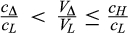
There is a continuum of customers indexed by type θ ∈ [0, 1]. Customers receive utility from the product based on their type, e.g., a customer type θ = 0.5 receives 0.5V _L and 0.5V _H utility from the original and new versions, respectively. We assume customer types are distributed uniformly on the unit interval. Customer segments are determined by type cut‐offs; for example, selling to customers with type θ ≥ θ ₁ in period one leaves a volume of x = (1 − θ ₁) new buyers in period two. There is no depreciation in the product, so the manufacturer's sales price of the original version in period two (if she continues its production) is the same as its price in the secondary market.⁹ The manufacturer and customers have discount factor δ for their second‐period payoffs. In line with Fudenberg and Tirole (1998), we also assume V _L > δV _Δ. This is a simplifying assumption—it does not rule out all high innovation levels, but restricts the very large ones—and is very helpful with some of the mathematical simplifications.

There are two cases regarding the market information: anonymous and semi‐anonymous. In the anonymous case, where the manufacturer does not keep track of former customers, customers can buy the new version by selling their current version in a frictionless external secondary market or to the manufacturer (when she offers to buy it back). In the semi‐anonymous case, the manufacturer is able to track the identity of the product owners, and thus she offers the new version to her former customers at a discounted price, called the upgrade price, less than its regular sales price. The anonymous case, wherein the manufacturer keeps buying back the customers’ old versions and selling them the new version separately, resembles a trade‐in frame. The semi‐anonymous case, on the other hand, wherein the manufacturer combines the two transactions into one net buying transaction for customers, is an upgrade frame.

We start with the upgrade frame. The manufacturer's optimization begins with her production‐pricing decision in period two, given the cut‐off θ ₁ from period one. Figure 1 shows the market segmentation. The θ _u is the cut‐off for the former customers’ type who decide to upgrade in period two. The upgrade price for these customers is p _u = θ _u V _Δ, coming from θ _u V _L − p _u = θ _u V _H. The θ _H and θ _L, on the other hand, are the cut‐offs for the new customers’ types who buy the new and original versions, respectively, in period two. It is straightforward to show that p _H = θ _L V _L + θ _H V _Δ and p _L = θ _L V _L.

Figure 1

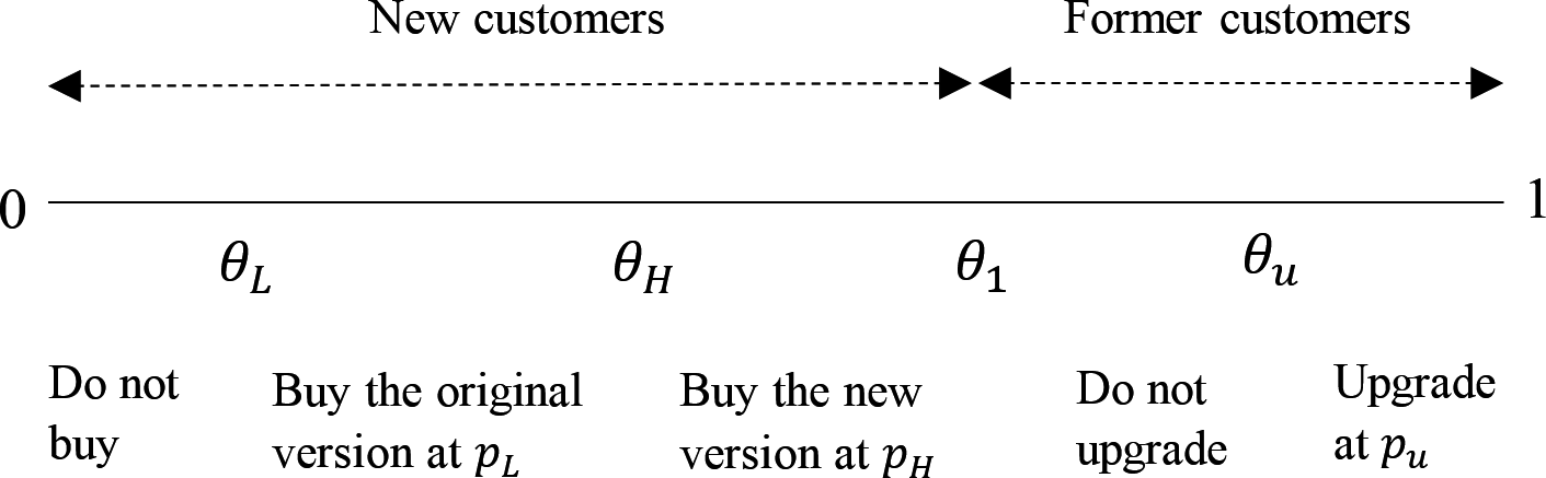
Market Segmentation with Upgrades

With the cut‐offs illustrated in Figure 1, the manufacturer's profit function in period two is as follows (note that c _L = 0):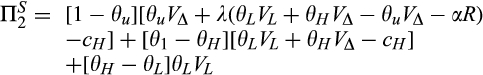

\begin{matrix} Π_{2}^{S} = & [1 - θ_{u}] [θ_{u} V_{Δ} + λ (θ_{L} V_{L} + θ_{H} V_{Δ} - θ_{u} V_{Δ} - α R) \\ - c_{H}] + [θ_{1} - θ_{H}] [θ_{L} V_{L} + θ_{H} V_{Δ} - c_{H}] \\ + [θ_{H} - θ_{L}] θ_{L} V_{L} \end{matrix}

(5)

where θ ₁ ≤ θ _u.

The constraint θ ₁ ≤ θ _u ensures that the volume of upgraders cannot be more than the volume of the sales in period one. The λ ≥ 0 is the reference‐dependence weight. With λ = 0, which implies no reference dependence, Equation 5 is identical to the classical model presented by Fudenberg and Tirole (1998). Therefore, with λ = 0, and for c _Δ = 0 (representing the high innovation case), we get their main result that the manufacturer will not continue production and sale of the original version in period two (and hence, p _H = θ _H V _H). The intuition behind this result lies in the perception that production and sale of the original version in the presence of a new version with high innovation is useless. The reference‐dependence model introduces an additional term, λ(θ _L V _L + θ _H V _Δ − θ _u V _Δ − αR), or equivalently λ(p _H − p _u − αR), embedded in the upgraders’ utility function, which represents their reference‐dependence behavior: p _H − p _u is what the upgraders receive for their current version, α ≥ 0 is the strength of anchoring to the reference point R (α = 0 means customers expect zero price for their current product and thus their reference‐point value is zero), and λ is the reference‐dependence weight. The reference dependence in Equation 5 has a simple interpretation: If the discount amount (i.e., p _H − p _u) is bigger than what the customers expect for their current version (i.e., p _H − p _u − αR > 0), it brings a gain for them. Thus, the manufacturer can charge them more (up to the amount p _u + λ[p _H − p _u − αR]) and still make the transaction happen. On the other hand, if the discount amount is lower than the customers’ reference‐point value and thus induces a loss for them (i.e., p _H − p _u − αR < 0), the manufacturer has to charge them less (i.e., p _u + λ(p _H − p _u − αR) < p _u) in order to make the upgrade happen. In light of what the reference dependence adds, there could be a value for the manufacturer in production and sale of the original version in period two. That is, if the manufacturer can manage the former customers’ reference points via the sales price of the original version, continuing its production and sale in period two is now not useless.

Based on the experimental results in Table 5, with an upgrade under a high innovation level in the new version, two situations can happen regarding the reference point: (i) customers anchor to the current sales price of their product, when the manufacturer sells the original version in period two, and (ii) customers anchor to the price they paid to purchase their product in period one, when the manufacturer does not continue its production and sale in period two. Given that the sales price of the original version in period two is significantly lower than its price in period one, and that customers may expect a price close to the current sales price of their product but will not expect a price very close to what they originally paid, it is plausible that customers’ anchoring parameter (α) to the original purchase price would be lower than that to the current sales price—this can also be inferred from Table 5. With this, we normalize α to α = 1 in customers’ anchoring to the current sales price of their product and to 0 < α < 1 in their anchoring to its original purchase price. This normalization remarkably simplifies the analysis and later the comparison between trade‐ins and upgrades. Furthermore, we assume λ = 1 regardless of gain or loss in the reference‐dependence term. This keeps the focus of our model extension on the reference dependence and ensures that our results are not driven by loss aversion (it is noted that considering λ _loss > λ _gain ≥ 1 does not bring any qualitative change in the results). With these, our behavioral model adds only one new parameter (0 < α < 1) to the existing model (see Long and Nasiry 2014 and Tong and Feiler 2016 for similar behavioral model extensions adding only one new parameter to an existing model).

For (i), and with α = 1, we replace αR in Equation 5 with θ _L V _L (i.e., the current sales price of the current version), which yields the manufacturer's second‐period profit function (for when she continues production and sale of the original version in period two) as follows: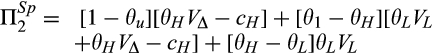

\begin{matrix} Π_{2}^{Sp} = & [1 - θ_{u}] [θ_{H} V_{Δ} - c_{H}] + [θ_{1} - θ_{H}] [θ_{L} V_{L} \\ + θ_{H} V_{Δ} - c_{H}] + [θ_{H} - θ_{L}] θ_{L} V_{L} \end{matrix}

(6)

where θ ₁≤θ _u.

Similarly, for (ii), and with 0 < α < 1, replacing αR with αp ₁ in Equation 5, we have the manufacturer's second‐period profit function (for when she does not continue production and sale of the original version in period two) as follows: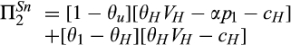

\begin{matrix} Π_{2}^{Sn} & = [1 - θ_{u}] [θ_{H} V_{H} - α p_{1} - c_{H}] \\ + [θ_{1} - θ_{H}] [θ_{H} V_{H} - c_{H}] \end{matrix}

(7)

where θ ₁ ≤ θ _u.

The manufacturer's first‐period profit comes from selling the original version to new buyers, and adding the second‐period profit to that shapes the manufacturer's total profit function, that is,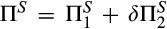

Π^{S} = Π_{1}^{S} + δ Π_{2}^{S}

(see Appendix D for deriving its mathematics). Comparing the manufacturer's total optimal profit with and without overlapping production in period two, we present the following proposition on the manufacturer's optimal strategy:

Proposition 1

In the semi‐anonymous case (i.e., with upgrades), under a high innovation level in the new version, for

α > \hat{α}

, the manufacturer is better off with overlapping production of the original version alongside the new version in period two.

The proof is available in Appendix D. Proposition 1 provides an opposite prediction to that of the classical model. The intuition behind Proposition 1 is straightforward and has roots in the rationale that the sale of the original version in period two can be useful in managing the upgraders’ reference points—that is, the manufacturer continues producing the original version and drops its price significantly to reduce the upgraders’ expectation as to the price for their current version. Hence, for α of sufficient magnitude, the reference‐point value under overlapping production (θ _L V _L) is lower than that under no overlapping production (αp ₁), and as a result, driven by the reference dependence, the manufacturer can charge a higher upgrade price by overlapping production than by not overlapping production. In addition, with overlapping production in period two, the manufacturer is not limited in charging higher sales prices for the original version in period one, as she now controls the upgrades’ reference points through her second‐period sales prices. This would, in turn, increase the first‐period profit for the manufacturer. Therefore, there are α′s for which the manufacturer is better off with overlapping production in period two. Figure 2 illustrates this by comparing the manufacturer's optimal profit under overlapping production with that under no overlapping production for all ranges of 0 ≤ α ≤ 1.

Figure 2

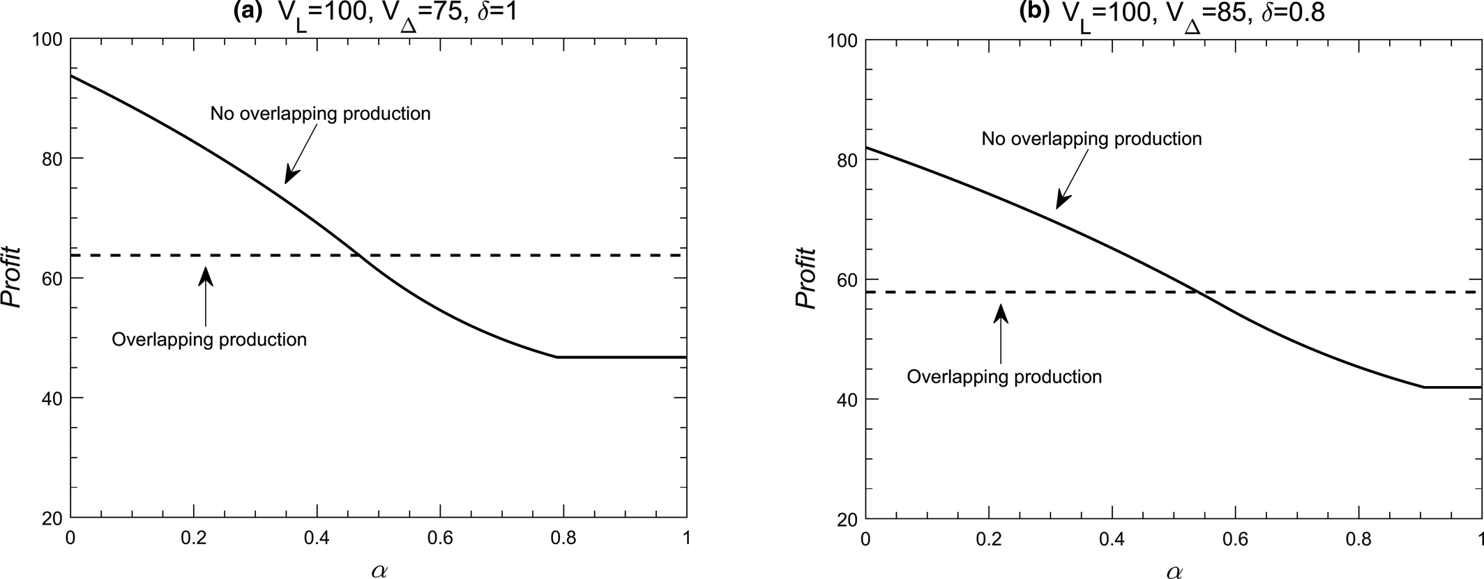
Manufacturer's Optimal Profit with Upgrades

Figure 3 depicts the optimal solution, that is, the optimal cut‐offs, under a “no overlapping production” scenario for 0 ≤ α ≤ 1. In the extreme case of α = 0, where former customers have no expectation as to a price for their current version and behave like new buyers in period two, the second period sales become independent from the first period sales, and as a result, all cut‐offs reach the optimal point of

θ^{*} = \frac{1}{2}

. This is very similar to a situation where the product's lifecycle is only one period. When α increases above zero, the manufacturer faces the upgraders’ expectation in period two. To manage that, she reduces the sales price in period one to keep the upgraders’ reference point low in period two. In addition, she keeps the new version's sales price high to induce a high discount price (i.e., p _H − p _u) to the upgraders. The former expands the manufacturer's sales in period one, and the latter hinders selling to new buyers in period two. Thus, the manufacturer only relies on the upgraders and does not sell to new buyers in period two. After a point, the manufacturer cannot keep the upgraders’ reference point at low levels because α is too high, nor can she handle the high reference point in period two by increasing the new version's sales price (to increase the induced discount price). Therefore, she starts relying on new buyers in period two; the bigger the α, the smaller the sales in period one and upgrades in period two, but the higher the sales to new buyers in period two. This is reached by setting a high cut‐off in period one (θ ₁) and a low cut‐off in period two (θ _H). For very high α ^′s, the manufacturer is not able to handle the upgraders’ reference point and hence starts relying only on new buyers in each period, where no upgrade happens in period two, and the manufacturer's optimal profit reaches a steady point.

Figure 3

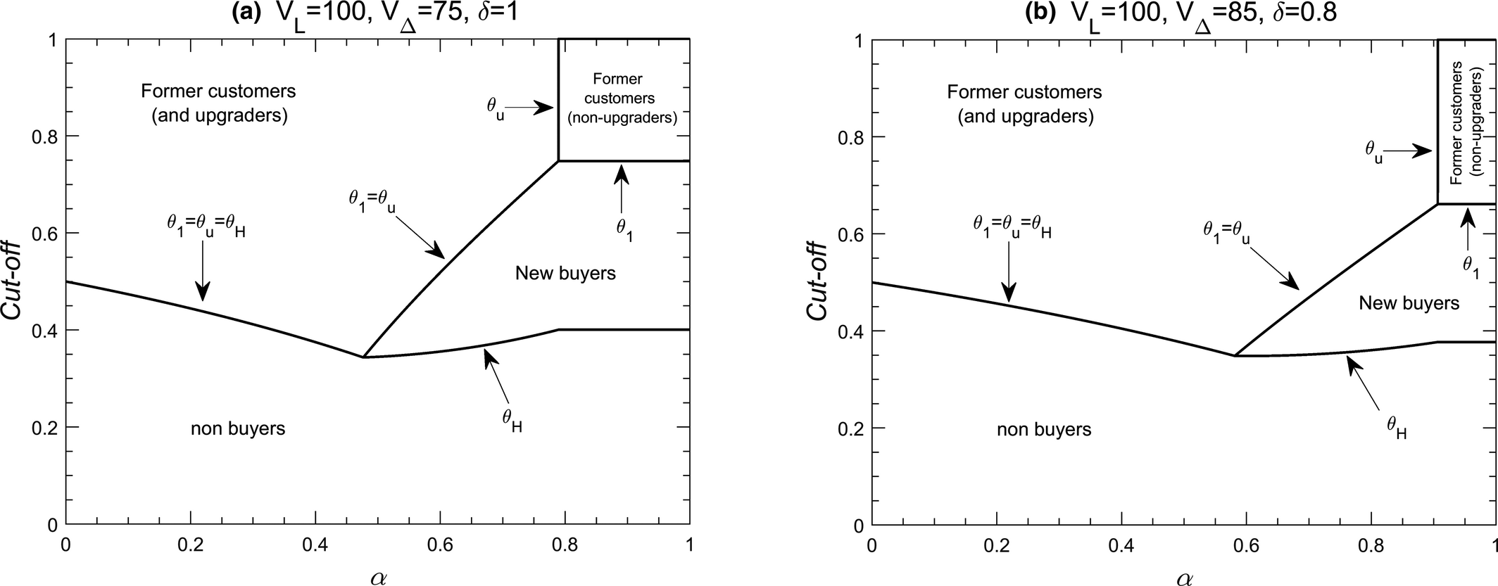
Manufacturer's Optimal Solution with Upgrades

We next analyze the model of trade‐ins in Fudenberg and Tirole (1998). Similar to the upgrade model, the manufacturer's optimization begins with her production‐pricing decision in period two, given the cut‐off θ ₁ from period one: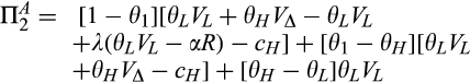

\begin{matrix} Π_{2}^{A} = & [1 - θ_{1}] [θ_{L} V_{L} + θ_{H} V_{Δ} - θ_{L} V_{L} \\ + λ (θ_{L} V_{L} - α R) - c_{H}] + [θ_{1} - θ_{H}] [θ_{L} V_{L} \\ + θ_{H} V_{Δ} - c_{H}] + [θ_{H} - θ_{L}] θ_{L} V_{L} \end{matrix}

(8)

The terms p _H = θ _L V _L + θ _H V _Δ and p _L = θ _L V _L are the second‐period prices for the new and original versions, respectively. The manufacturer sells the new version to all customers (i.e., replacement buyers and new buyers) at the regular sales price θ _L V _L + θ _H V _Δ; she sells the original version to new buyers at price θ _L V _L and, because of no depreciation in the product, buys it back from the replacement buyers at the same price θ _L V _L. The λ ≥ 0 and α ≥ 0 have the same meanings as in Equation 5. With λ = 0, that is, no reference dependence, Equation 8 is identical to the classical model by Fudenberg and Tirole (1998), and c _Δ = 0 (representing the high innovation case) yields their main result that the manufacturer does not continue production and sale of the original version in period two.¹⁰ The reference‐dependence term in Equation 8 modifies the replacement buyers’ utility function and has a similar interpretation to that in Equation 5: If the price paid for the customers’ current version is higher than what they expect it to be (i.e., θ _L V _L > αR), they feel a gain in the amount of λ[θ _L V _L − αR]. Thus, the manufacturer can reduce the price she pays to replacement buyers for their current version (i.e., θ _L V _L − λ[θ _L V _L − αR]) and still make the trade‐in happen. Note that the manufacturer can also increase the new version's price (i.e., θ _L V _L + θ _H V _Δ) in taking advantage of θ _L V _L > αR; however, she is limited in doing so because it causes her to lose the new buyers segment.

Based on the experimental results in Table 5, with trade‐ins, customers anchor to the secondary market price as their reference point, regardless of the new version's innovation level or the manufacturer's decision whether to continue production and sale of the original version in period two. Hence, with α = 1 (driven by Fudenberg and Tirole's assumption of no depreciation in the product and that the secondary market price of the original version is the same as its sales price in period two when the manufacturer continues its production and sale; see Footnote 9), we replace αR in Equation 7 with θ _L V _L. This results in λ(θ _L V _L − αR) = λ(θ _L V _L − θ _L V _L) = 0. Thus, we have the manufacturer's profit function in period two as follows: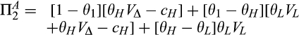

\begin{matrix} Π_{2}^{A} = & [1 - θ_{1}] [θ_{H} V_{Δ} - c_{H}] + [θ_{1} - θ_{H}] [θ_{L} V_{L} \\ + θ_{H} V_{Δ} - c_{H}] + [θ_{H} - θ_{L}] θ_{L} V_{L} \end{matrix}

(9)

The manufacturer's total profit function is

Π^{A} = Π_{1}^{A} + δ Π_{2}^{A}

(see Appendix D for deriving its mathematics), where

Π_{1}^{A}

is her first‐period profit from selling the original version to new buyers. Based on what we obtained in Equation 9, with α = 1, the reference‐dependence model here coincides with the classical model. Thus, Fudenberg and Tirole (1998) main result here, that is, no production and sale of the original version in period two, holds with the reference‐dependence model, as well. In comparing trade‐ins and upgrades, however, the anomaly between the predictions of the classical model and those of the reference‐dependence model for the latter brings us to the following proposition:

Proposition 2

Under a high innovation level in the new version, for

α < \hat{α}

, the manufacturer is better off in the semi‐anonymous case (i.e., with upgrades) than in the anonymous case (i.e., with trade‐ins). For

α \geq \hat{α}

, both yield the same optimal profit through the same optimal pricing.

Proposition 2 is in stark contrast with the classical model, which favors the anonymous case (and trade‐ins).¹¹ The intuition behind Proposition 2 roots back in the previous result presented in Proposition 1, where the overlapping production becomes the optimal strategy for

α \geq \hat{α}

. The overlapping production with upgrades pushes the optimal solution closer to the commitment solution by creating the cut‐off θ _L in period two. In other words, through managing the upgraders’ reference points, the manufacturer indirectly pursues a policy that creates Coasian dynamics (similar to when monopolists create Coasian dynamics through unconventional methods, such as introducing damaged versions of their durable goods to the market; see, e.g., Hahn 2006). Furthermore, because for

α \geq \hat{α}

, the reference point is θ _L V _L with both trade‐ins and upgrades, they yield the same optimal pricing and thus the same optimal profit (the mathematical proof of this is provided in Appendix D). That being said, the baseline profit in Figure 2 represents the optimal profit with trade‐ins, as well. As seen, for

α < \hat{α}

, the upgrade frame yields more profit than the baseline because of its reference point being very low, and for

α \geq \hat{α}

, the manufacturer can always obtain the baseline profit by switching to overlapping production.

Concluding Remarks

In this study, we examined whether the conventional wisdom that trade‐ins and upgrades are equivalent was robust to behavioral influences. Using the reference‐point shift mechanism, our study yielded two main results. First, experimental analyses established that customers change which prices they anchor to as their reference points when offered a trade‐in or upgrade and that different market settings have different effects with the two frames in terms of shifting customers’ reference points, depending on which price anchor they change. Second, the reference‐point shift of the sort revealed here modify predictions of the classical model of trade‐ins and upgrades and provide predictions more in line with today's durable goods markets. In particular, we find that manufacturers may prefer to produce older versions of their products concurrently with newer, improved versions even in settings where the classical model predicts they would not. The addition of reference dependence to the classical model, therefore, can explain observed co‐production of successive versions of products that cannot be explained by the classical model. This modification further contradicts the classical model's outcome in comparing trade‐ins and upgrades and shows that the dominant profitability of trade‐ins predicted by the classical model is not the case.

Our findings have obvious implications for manufacturers of durable goods that offer replacement purchases for their former customers. The choice between offering a trade‐in or upgrade influences customers’ choice of the reference point for the price for their current version. Hence, manufacturers can choose the frame to direct their customers’ focus away from low‐profit reference points and towards more profitable ones. Because switching between frames is likely to be a low‐cost tactic for most manufacturers, the framing effect offers a flexible tool in managing former customers in a profitable way. Finding the optimal frame and the optimal production‐pricing policy in each market setting was beyond the scope of this study. Nonetheless, our experiment covered all possible market settings in line with the seminal framework of trade‐ins and upgrades in order to provide inputs for future analytical research in this area. In this study, we set our problem setting with that of Fudenberg and Tirole (1998) that is for a monopoly manufacturer. While such settings are justified in the literature of durable goods (Waldman 2003), future studies facing perfect substitution between products can also consider competitors’ prices, alongside other potential price anchors, in the problem setting. Such settings would allow factoring in propensity for brand switching in replacement buyers’ decisions by considering two competitor manufacturers introducing sequential versions of perfectly substitutable products.

Footnotes

Experimental Materials

Full Regression Models

Further Analyses

Proofs

Acknowledgments

The author is grateful to his dissertation advisor, Peter Thompson, for his helpful comments and feedback on this study. The author also thanks the review team for their constructive comments and suggestions.

1

Indeed, Ray et al. () showed that by offering different prices for replacement and new buyers, manufacturers could increase their profit by up to 40%.

2

Sony continued production of the PS3 until September 2015, over one year after the PS4 was released. The PS3 was not compatible with the PS4, which came with major (and unique) innovations, such as integrated social gaming services.

3

Indeed, Hossain and List () emphasize the existence of the framing effect in real‐life decision‐making in addition to experimental settings.

4

As discussed by Waldman (2003), most durable goods manufacturers, though not being monopolists, do have a market power that resembles a monopoly because there is almost no perfect substitution for any product. Therefore, we keep our focus on the potential price anchors in Fudenberg and Tirole () monopoly framework and do not bring competitors’ prices as further price anchors. We use, however, the average secondary market price in our experimental study to account for the possibility of multiple prices in the external secondary market.

5

The ordering was random and counterbalanced. In addition, to ensure the reliability of the results from using the same participants for both innovation levels, we performed a robustness check by considering only the first question that the participants answered and obtained the same results (see Appendix C).

6

Similar to pre‐filtering of participants in lab experiments with test rounds, our attention‐check question is to filter participants who failed to pay attention to the descriptions. We report the whole collected data because our attention‐check question was set at the end of the experiment after the participants took the main experimental task. Pre‐exclusion of these participants results in a data loss of < 4.7% through filtering the outlier responses. While our main results are robust to including the outlier responses in the sample, we exclude them from the analysis to ensure quantitative reliability of the regression results.

7

With including the order as another between‐subject factor, our mixed model is thus practically a 2 × 4 × 2 × 2 design. It is also worth noting that including the participants’ demographics (e.g., age, gender, etc.) as further control factors makes no difference in the results either, and the observed effects are independent of the participants’ demographics.

8

It is noted that because the column‐wise comparisons were over the same participants, in order to account for possible correlations in error terms, we also used z‐tests with Seemingly Unrelated Estimation and found the same results.

9

This assumption of Fudenberg and Tirole (), though not being realistic, does not bring any qualitative shortfalls in the model and its results, while significantly simplifying the analysis. The otherwise is just a matter of depreciation parameters and making quantitative changes. Hence, we keep this assumption in our behavioral extension, as well, and assume no depreciation (or depreciation rate =1) in our model and analysis. It is noted that because our experimental design was with a secondary market price less than the sales price, our extension does allow depreciation (through adding a depreciation parameter < 1) if one wishes to expand Fudenberg and Tirole (1998) model in that direction in the interest of quantitative analyses.

10

Note that although the manufacturer does not produce and sell the original version in period two, new customers can still buy it from the secondary market, and hence there always exists a cut‐off θ _L for those customers, and the new version's price always takes the form of p _H = θ _L V _L + θ _H V _Δ not p _H = θ _H V _H.

11

The intuition behind this result of the classical model is that because of not pricing the original version in period two in the semi‐anonymous case (i.e., with upgrades), the new version's sales price falls below the commitment price, and hence the manufacturer never reaches the commitment solution. However, the secondary market price in the anonymous case (i.e., with trade‐ins), which creates the cut‐off θ _L for the original version in period two, pushes the cut‐off θ _H upward, which, in turn, helps the manufacturer get closer to the commitment solution.

References

Abbey

J. D.

Meloy

M. G.

. 2017. Attention by design: Using attention checks to detect inattentive respondents and improve data quality. J. Oper. Manag. 53: 63–70.

Agrawal

Ferguson

Souza

G. C.

. 2016. Trade‐in rebates for price discrimination and product recovery. IEEE Trans. Eng. Manag. 63(3): 326–339.

Appleinsider . 2016. Apple R&D spending jumps to $2.5B in Q2, accounted for 5% of total revenue. appleinsider.com (April 27). Available at http://appleinsider.com/articles/16/04/27/apple-rd-spending-jumps-to-25b-in-q2-accounted-for-5-of-total-revenue/ (accessed date June 2, 2017).

Baucells

Weber

Welfens

. 2011. Reference‐point formation and updating. Management Sci. 57(3): 506–519.

Benjamin

D. K.

Kormendi

R. C.

. 1974. The interrelationship between markets for new and used durable goods. J. Law Econ. 17(2): 381–401.

Carmon

Ariely

. 2000. Focusing on the forgone: How value can appear so different to buyers and sellers. J. Consum. Res. 27(3): 360–370.

Chen

Esteban

Shum

. 2013. When do secondary markets harm firms? Am. Econ. Rev. 103(7): 2911–2934.

Cheng

P.‐Y.

Chiou

W.‐B.

. 2008. Framing effects in group investment decision making: Role of group polarization. Psychol. Rep. 102(1): 283–292.

Clogg

C. C.

Petkova

Haritou

. 1995. Statistical methods for comparing regression coefficients between models. Am. J. Sociol. 100(5): 1261–1293.

10.

Dutta

Das

Schultmann

Fröhling

. 2016. Design and planning of a closed‐loop supply chain with three way recovery and buy‐back offer. J. Clean. Prod. 135: 604–619.

11.

Fishman

Rob

. 2000. Product innovation by a durable‐good monopoly. Rand J. Econ. 31(2): 237–252.

12.

Fudenberg

Tirole

. 1998. Upgrades, tradeins, and buybacks. Rand J. Econ. 29(2): 235–258.

13.

Gächter

Orzen

Renner

Starmer

. 2009. Are experimental economists prone to framing effects? A natural field experiment. J. Econ. Behav. Org. 70(3): 443–446.

14.

Gallagher

K. M.

Updegraff

J. A.

. 2012. Health message framing effects on attitudes, intentions, and behavior: a meta‐analytic review. Ann. Behav. Med. 43(1): 101–116.

15.

Golson

2016. More than half of iPhone users haven’t upgraded to a 6 or 6s yet. Yahoo Tech (January 26). Available at http://www.yahoo.com/tech/more-half-iphone-users-haven-003807335.html (accessed date June 2, 2017).

16.

Gordon

B. R.

2009. A dynamic model of consumer replacement cycles in the PC processor industry. Mark. Sci. 28(5): 846–867.

17.

Guide

V. D. R.

Wassenhove

L. N.

. 2001. Managing product returns for remanufacturing. Prod. Oper. Manag. 10(2): 142–155.

18.

Guiltinan

2010. Consumer durables replacement decision‐making: An overview and research agenda. Mark. Lett. 21(2): 163–174.

19.

Hahn

J.‐H.

2006. Damaged durable goods. Rand J. Econ. 37(1): 121–133.

20.

Hannan

R. L.

Hoffman

V. B.

Moser

D. V.

, 2005. Bonus versus penalty: Does contract frame affect employee effort? In: Experimental Business Research. Springer, Boston, 151–169.

21.

Hardisty

D. J.

Pfeffer

. 2016. Intertemporal uncertainty avoidance: When the future is uncertain, people prefer the present, and when the present is uncertain, people prefer the future. Management Sci. 63(2): 519–527.

22.

Hauser

D. J.

Schwarz

. 2016. Attentive turkers: Mturk participants perform better on online attention checks than do subject pool participants. Behav. Res. Methods 48(1): 400–407.

23.

Heath

T. B.

Chatterjee

France

K. R.

. 1995. Mental accounting and changes in price: The frame dependence of reference dependence. J. Consum. Res. 22(1): 90–97.

24.

Hendel

Lizzeri

. 1999. Interfering with secondary markets. Rand J. Econ. 30(1): 1–21.

25.

T.‐H.

Zhang

. 2008. Designing pricing contracts for boundedly rational customers: Does the framing of the fixed fee matter? Management Sci. 54(4): 686–700.

26.

Hossain

List

J. A.

. 2012. The behavioralist visits the factory: Increasing productivity using simple framing manipulations. Management Sci. 58(12): 2151–2167.

27.

Hoyer

W. D.

Herrmann

Huber

. 2002. When buyers also sell: The implications of pricing policies for customer satisfaction. Psychol. Mark. 19(4): 329–355.

28.

Kim

Rao

R. S.

Kim

Rao

A. R.

. 2011. More or less: A model and empirical evidence on preferences for under‐ and overpayment in trade‐in transactions. J. Mark. Res. 48(1): 157–171.

29.

Kohler

2016. Soon you’ll buy Consoles the way you upgrade iPhones. Wired (May 26). Available at http://www.wired.com/2016/05/future-of-game-consoles/ (accessed date June 2, 2017).

30.

Kornish

L. J.

2001. Pricing for a durable‐goods monopolist under rapid sequential innovation. Management Sci. 47(11): 1552–1561.

31.

Ko˝szegi

Rabin

. 2006. A model of reference‐dependent preferences. Quart. J. Econ. 121(4): 1133–1165.

32.

Kumar

Lim

S. S.

. 2008. How do decision frames influence the stock investment choices of individual investors? Management Sci. 54(6): 1052–1064.

33.

Lee

Y. S.

Seo

Y. W.

Siemsen

. 2018. Running behavioral operations experiments using amazon's mechanical turk. Prod. Oper. Manag. 27(5): 973–989.

34.

Lehner

J. M.

2000. Shifts of reference points for framing of strategic decisions and changing risk‐return associations. Management Sci. 46(1): 63–76.

35.

Levinthal

D. A.

Purohit

. 1989. Durable goods and product obsolescence. Mark. Sci. 8(1): 35–56.

36.

K. J.

Fong

D. K.

S. H.

. 2011. Managing trade‐in programs based on product characteristics and customer heterogeneity in business‐to‐business markets. Manuf. Serv. Oper. Manag. 13(1): 108–123.

37.

Liebowitz

S. J.

1985. Copying and indirect appropriability: Photocopying of journals. J. Polit. Econ. 93(5): 945–957.

38.

Lim

T.‐H.

. 2007. Designing price contracts for boundedly rational customers: Does the number of blocks matter? Mark. Sci. 26(3): 312–326.

39.

Long

Nasiry

. 2014. Prospect theory explains newsvendor behavior: The role of reference points. Management Sci. 61(12): 3009–3012.

40.

Luft

1994. Bonus and penalty incentives contract choice by employees. J. Acc. Econ. 18(2): 181–206.

41.

Monga

Zhu

R. J.

. 2005. Buyers versus sellers: How they differ in their responses to framed outcomes. J. Consum. Psychol. 15(4): 325–333.

42.

Okada

E. M.

2001. Trade‐ins, mental accounting, and product replacement decisions. J. Consum. Res. 27(4): 433–446.

43.

Okada

E. M.

2006. Upgrades and new purchases. J. Mark. 70(4): 92–102.

44.

Oraiopoulos

Ferguson

M. E.

Toktay

L. B.

. 2012. Relicensing as a secondary market strategy. Management Sci. 58(5): 1022–1037.

45.

Purohit

1995. Playing the role of buyer and seller: The mental accounting of trade‐ins. Mark. Lett. 6(2): 101–110.

46.

Rabin

2013a. An approach to incorporating psychology into economics. Am. Econ. Rev. 103(3): 617–622.

47.

Rabin

2013b. Incorporating limited rationality into economics. J. Econ. Lit. 51(2): 528–543.

48.

Rao

R. S.

Narasimhan

John

. 2009. Understanding the role of trade‐ins in durable goods markets: Theory and evidence. Mark. Sci. 28(5): 950–967.

49.

Ray

Boyaci

Aras

. 2005. Optimal prices and trade‐in rebates for durable, remanufacturable products. Manuf. Serv. Oper. Manag. 7(3): 208–228.

50.

Rust

1986. When is it optimal to kill off the market for used durable goods? Econometrica 54(1): 65–86.

51.

Seo

2006. A review and comparison of methods for detecting outliers in univariate data sets. Ph.D. thesis, University of Pittsburgh.

52.

Simonson

Drolet

. 2004. Anchoring effects on consumers’ willingness‐to‐pay and willingness‐to‐accept. J. Consum. Res. 31(3): 681–690.

53.

Souza

G. C.

2013. Closed‐loop supply chains: A critical review, and future research. Decis. Sci. 44(1): 7–38.

54.

Srivastava

Chakravarti

. 2011. Price presentation effects in purchases involving trade‐ins. J. Mark. Res. 48(5): 910–919.

55.

Statista , 2014. By next year 80% of iPhone sales could be replacements. statista.com (March 13). Available at http://statista.com/chart/1999/iphone-sales-by-type-of-purchase/ (accessed date June 2, 2017).

56.

Statisticbrain , 2016. iPhone 5 sales statistics. statisticbrain.com (September 26). Available at http://www.statisticbrain.com/iphone-5-sales-statistics/ (accessed date June 2, 2017).

57.

Tang

C. S.

Zhou

. 2012. Research advances in environmentally and socially sustainable operations. Eur. J. Oper. Res. 223(3): 585–594.

58.

Thaler

1980. Toward a positive theory of consumer choice. J. Econ. Behav. Org. 1(1): 39–60.

59.

Thaler

1985. Mental accounting and consumer choice. Marketing science 4(3): 199–214.

60.

Time , 2014. Apple's $649 iPhone 6 reportedly costs $200 to make. time.com (September 24). Available at http://time.com/3426087/apple-iphone-6-cost/ (accessed date June 2, 2017).

61.

Time , 2016. The iPhone 7 costs you 3x more than it costs Apple to make. time.com (September 26). Available at http://time.com/money/4508221/iphone-7-mark-up-profit-margins/ (accessed date June 2, 2017).

62.

Tong

Feiler

. 2016. A behavioral model of forecasting: Naïve statistics on mental samples. Management Sci. 63(11): 3609–3627.

63.

Tversky

1977. Features of similarity. Psychol. Rev. 84(4): 327–352.

64.

Tversky

Kahneman

. 1981. The framing of decisions and the psychology of choice. Science 211(4481): 453–458.

65.

Tversky

Kahneman

. 1986. Rational choice and the framing of decisions. J. Bus. 59(4): S251–S278.

66.

Tversky

Kahneman

. 1991. Loss aversion in riskless choice: A reference‐dependent model. Quart. J. Econ. 106(4): 1039–1061.

67.

Van Ackere

Reyniers

D. J.

. 1993. A rationale for trade‐ins. J. Econ. Bus. 45(1): 1–16.

68.

Van Ackere

Reyniers

D. J.

. 1995. Trade‐ins and introductory offers in a monopoly. Rand J. Econ. 26(1): 58–74.

69.

Waldman

1996. Planned obsolescence and the R&D decision. Rand J. Econ. 27(3): 583–595.

70.

Waldman

. 2003. Durable goods theory for real world markets. J. Econom. Perspect. 17(1): 131–154.

71.

Yang

Vosgerau

Loewenstein

. 2013. Framing influences willingness to pay but not willingness to accept. J. Mark. Res. 50(6): 725–738.

72.

Zhang

. 2018. Trade‐in remanufacturing, customer purchasing behavior, and government policy. Manuf. Serv. Oper. Manag. 20(4): 601–616.

73.

Zhao

Jagpal

. 2009. Upgrade pricing, market growth, and social welfare. J. Bus. Res. 62(7): 713–718.

74.

Zhu

Chen

Dasgupta

. 2008. Can trade‐ins hurt you? Exploring the effect of a trade‐in on consumers’ willingness to pay for a new product. J. Mark. Res. 45(2): 159–170.