
Abstract
Many manufacturing and service systems require a finite number of heterogeneous jobs to be processed by two stations in tandem. Each station serves at most one job at a time and there is a finite buffer between the two stations. We consider two flexible servers that are cross‐trained to work at both stations. The duration for a server to finish a job at a station is exponentially distributed with a rate that depends on the server, the station, and the job. Our goal is to identify an efficient policy to dynamically assign the servers to the stations such that the expected makespan (duration to complete all the jobs) is minimized. Given that an optimal policy is non‐idling, we focus on non‐idling policies. We first derive the expected makespan of a general non‐idling policy. We then analyze three simple non‐idling policies: the summation‐myopic, the product‐myopic, and the teamwork policies. We prove that (i) the product‐myopic policy is optimal if the servers maintain the same service‐rate ratio at each station for all the jobs, (ii) the teamwork policy is optimal if the servers maintain the same service‐rate ratio at different stations for jobs that are sequenced near each other, and (iii) the summation‐myopic policy is no worse than the teamwork policy. Our numerical study based on general service rates suggests that the summation‐myopic policy can be better or worse than the product‐myopic policy. We also extend the model to incorporate moving costs and service defects.
Introduction
A tandem system consists of a sequence of work stations. Servers work on jobs that go through the stations sequentially. The value of each job increases as it progresses from the start to the end of the tandem system. Tandem systems are common in the manufacturing industry (Hopp and Spearman 2008). For example, workers (servers) in a tandem system transform raw materials into finished goods in a production plant. Tandem systems can also be found in the service industry (Cachon and Terwiesch 2013). For instance, in a hospital, a tandem system diagnoses patients (jobs) through a sequence of medical tests. Since the labor cost constitutes a substantial portion of the operating cost in these environments, it is important to effectively make use of a tandem system's workforce to maximize its productivity.
We consider a tandem system with two stations shown in Figure . Each station can serve at most one job at a time. There are M < ∞ jobs available at an initial position in front of station 1 to be served by the tandem system. We consider only a finite number of jobs to be served by the system because this is quite common in practice. For example, the number of patients that visit a hospital for medical tests is finite every day. There is a buffer of size B between the two stations. Every job is first served by station 1. Upon completion at station 1, the job enters station 2 if the latter is available. Otherwise, the job either enters the buffer (if the buffer is not full) or stays at station 1 (if the buffer is full). There are at most B + 1 jobs waiting to enter station 2. The jobs maintain the same sequence as they go through the system.
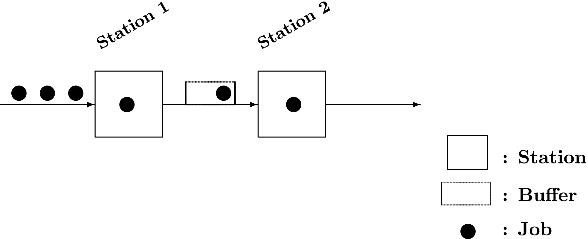
A Tandem System with Two Stations, Two Servers, and a Finite Number of Jobs
There are two flexible servers that are cross‐trained to work at both stations. Each server can work at only one station at a time. After he finishes a job he can move to another station, which takes negligible time and cost. We assume that the duration for a server to finish a job at a station is exponentially distributed with a rate that depends on the server, the station, and the job. Thus, the jobs are heterogeneous because they may have different service‐time distributions even if they are served by the same server at the same station. Furthermore, we assume that the two servers can work together on the same job at the same station simultaneously with additive service rates (Andradóttir et al. 2001).
Define makespan as the duration to complete all the jobs of the system. Our objective is to identify an efficient policy to dynamically assign the servers to the stations such that the expected makespan is minimized.
We describe the contributions of this study in the following paragraphs. To minimize the expected makespan, we formulate a stochastic dynamic program for B = 1 to find an optimal policy that dynamically assigns the servers to the stations. Unfortunately, the optimal policy is too complicated to characterize when the number of jobs M is large. This motivates us to develop simpler and more intuitive policies in this paper. We will use the optimal policy derived from the dynamic program as a benchmark when we evaluate these simpler policies. Since the optimal policy is non‐idling, we focus on non‐idling policies in this paper. Using the basic probability theory, we first derive the expected makespan of a system with a buffer size B = 1 under a general non‐idling policy. To the best of our understanding, this is the first paper performing such an analysis. We then study three specific non‐idling policies: the summation‐myopic policy, the product‐myopic policy, and the teamwork policy. The first two policies are developed by us and the last policy was proposed by Van Oyen et al. (2001).
The summation‐myopic policy chooses an assignment that maximizes the sum of the servers’ service rates for the current state of the system. The product‐myopic policy chooses an assignment that maximizes the product of the service rates at the two stations for the current state of the system. This policy generalizes the policy in Theorem 4.1 by Andradóttir et al. (2001) to a system with heterogeneous jobs. Under the teamwork policy (Van Oyen et al. 2001), all the servers work as a single team that follows each job from station 1 to station 2, and only starts working on a new job after the current job is completed. This policy is straightforward to implement in practice and no buffer is needed between the stations. We prove that each of these specific non‐idling policies is optimal under certain conditions on the service rates. We then conduct a numerical study to compare these non‐idling policies for general service rates. We extend the analysis to a system with a general buffer size

After reviewing the literature in section 2, we formulate the problem for B = 1 as a stochastic dynamic program in section 3. Section 4 derives the expected makespan of a system with B = 1 under a general non‐idling policy. Section 5 describes the three specific non‐idling policies and their expected makespan. Section 6 discusses the optimality conditions of these non‐idling policies, and compares the policies against the optimal one derived from the dynamic program. Section 7 extends the analysis to a system with a general buffer size

Related Literature
This study is related to two streams of literature: dynamic server assignment and dynamic line balancing. We discuss each stream of literature as follows.
Dynamic Server Assignment
There exists a stream of research focusing on dynamic server assignment policies that minimize holding costs. Many papers in this stream consider parallel or tandem queues with two stations. For example, Harrison and López (1999), Williams (2000), Bell and Williams (2001), Ahn et al. (2004), and Mandelbaum and Stolyar (2004) study flexible servers in parallel queues. On the other hand, Rosberg et al. (1982), Farrar (1993), Iravani et al. (1997), Duenyas et al. (1998), Kaufman et al. (2005), and Armony et al. (2018) study flexible servers in tandem queues. In contrast, our objective is to minimize the expected makespan.
Some papers identify dynamic server assignment policies that maximize throughput of tandem lines with finite buffers. Andradóttir et al. (2001) consider a two‐station, two‐server Markovian system that has an infinite supply of jobs in front of station 1. They assume that the service rates are independent of the jobs (that is, the jobs are homogeneous). They identify an optimal server assignment policy that maximizes the long‐run average throughput. The authors also propose near‐optimal heuristic policies for larger systems. Note that the product‐myopic policy generalizes their optimal policy to a system with heterogeneous jobs.
Andradóttir and Ayhan (2005) focus on the case with two stations and study the optimal server assignment policies for Markovian systems with more servers than the stations. Kirkizlar et al. (2010) show that the optimal or near‐optimal policies in Andradóttir et al. (2001) and Andradóttir and Ayhan (2005) for Markovian systems are also effective for non‐Markovian systems. Andradóttir et al. (2003) and Andradóttir et al. (2007a) study general queueing networks with infinite buffers without or with server and station failures. In contrast to this stream of research, we consider a finite supply of jobs for the system and assume the service rates depend on the jobs.
Andradóttir et al. (2007b) demonstrate that a Markovian system with two stations and generalist servers can attain most of the benefits of full flexibility by having only one flexible server when the buffer size is sufficiently large. Hopp et al. (2004) consider a line with an equal number of stations and servers under a constant work‐in‐process policy. They show that a skill‐chaining strategy with two skills per server can outperform a “cherry picking” strategy in which some servers are cross‐trained at bottleneck stations. Andradóttir et al. (2003) show that partial flexibility is sufficient for achieving the maximal capacity for a queueing network with outside arrivals and infinite buffers. Wallace and Whitt (2005) study routing and server assignment in a call center. They show that most of the benefits of full flexibility can be achieved even with one additional skill per agent. In contrast, we assume full flexibility such that each server is cross‐trained to serve at both stations. For a comprehensive review on cross‐trained workforce, see Hopp and Van Oyen (2004).
Dynamic Line Balancing
Another stream of research studies the dynamic line‐balancing problem with flexible servers. Bartholdi and Eisenstein (1996) analyze a bucket brigade system in which each server assembles a product along a flow line until either his colleague downstream takes over his work or he finishes his work at the end of the line; then he walks back to get more work, either from his colleague upstream or from a buffer at the start of the line. The authors show that if the servers are sequenced from slowest to fastest in the direction of production flow, then the system can achieve a maximum attainable throughput and a stable partition of work among the servers.
Bartholdi et al. (1999) study the long‐run behavior of bucket brigades with two to three servers. Bartholdi et al. (2001) study the performance of bucket brigades on discrete tasks with exponentially distributed service requirements. Bartholdi and Eisenstein (2005) consider a bucket brigade with walk‐back and hand‐off times. Armbruster and Gel (2006) study a bucket brigade where servers’ service rates do not dominate each other. Lim and Yang (2009) study bucket brigades on discrete work stations and find the policies that maximize the system's throughput.
To reduce the servers’ unproductive travel, Lim (2011) introduces the cellular bucket brigades, where each server works on one side of an aisle when he proceeds in one direction and works on the other side of the aisle when he proceeds in the reverse direction. The author demonstrates that a cellular bucket brigade can be 30% more productive than a traditional, serial bucket brigade. Lim (2017) studies the performance of cellular bucket brigades with hand‐off times. Lim and Wu (2014) study cellular bucket brigades on U‐lines with discrete work stations. For the line‐balancing problem in other tandem systems, see Ostolaza et al. (1990), Zavadlav et al. (1996), and Gel et al. (2002). Most of the papers in this stream of work maximize the system's throughput. Again, they assume an infinite supply of jobs for the system and the service rates are independent of the jobs.
Problem Formulation for Buffer Size B = 1
We first study a system with buffer size B = 1. Assume the time duration for server i to serve job m at station j is exponentially distributed with rate

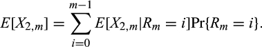
We assume that at time t = 0, both servers work on job 1 at station 1. Whenever a job is finished at a station, a server assignment policy instructs each server where to work next: station 1 or station 2. Let D m denote the departure time of job m from the system, and let E[D m ] denote its expected value. The objective of the problem is to find a server assignment policy that minimizes the expected makespanE[D M ], which represents the expected time duration to complete all the M jobs. A server assignment policy is optimal if it minimizes the expected makespan. It is straightforward to show that each server must be non‐idling at any time under an optimal server assignment policy. Therefore, we only focus on non‐idling policies that make both servers always busy until they complete the M jobs. At any instant under a non‐idling policy, there are four possible server assignments: (i) both servers at station 1, (ii) both servers at station 2, (iii) server 1 at station 1 and server 2 at station 2, and (iv) server 1 at station 2 and server 2 at station 1.
At time t, let U(t) denote the number of jobs that are not yet finished at station 1. We have U(t) ∈ {0,1,…,M}. Let V(t) denote the number of jobs that are finished at station 1 but not yet finished at station 2. We have V(t) ∈ {0,1,…,3}. Note that U(t) + V(t) ≤ M. Assume that at t = 0, all the M jobs are available at the initial position in front of station 1. Thus, given U(t) and V(t), we know exactly the locations of all the jobs. For example, (U(t),V(t)) = (6,2) implies that jobs M,M − 1,…,M − 4 are at the initial position, job M − 5 is at station 1, job M − 6 is at the buffer, job M − 7 is at station 2, and all the other jobs are completed and have left the system. Since service times are exponentially distributed and therefore memoryless, we define the state of the system as (U(t),V(t)).
For some special system states, it is straightforward to identify an optimal server assignment. (i) If V(t) = 0 (station 2 is starved), then it is optimal to assign both servers to station 1. (ii) If V(t) = 3 (station 1 is blocked) or U(t) = 0 (no more jobs to be served at station 1), then it is optimal to assign both servers to station 2. Thus, we only need to study the server assignment for other system states. For any state (u,v), let f (u,v) be the minimum expected time duration to serve all the remaining jobs in the system. The problem can be formulated as a stochastic dynamic program shown in Table .
Dynamic Programming Formulation for a System with a Buffer Size B = 1
Note that 


We can obtain the optimal policy by solving the dynamic program in Table 1. The expected makespan under the optimal policy is f (M,0). However, it is difficult to analytically characterize the structure of the optimal policy because of its complexity in general. Thus, it is hard to implement the optimal policy in practice, which motivates us to study simpler and more intuitive policies. In the following sections, we first determine the expected makespan of a general non‐idling policy. We then focus on three specific non‐idling policies, and benchmark their performance against the optimal policy.
The Expected Makespan of a General Non‐Idling Policy for Buffer Size B = 1
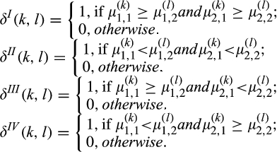
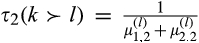
In this section, we determine the expected makespan under a general non‐idling policy for buffer size B = 1. Suppose jobs k and l are at stations 1 and 2 respectively. There are two possible cases. In case (i), job k finishes service at station 1 before job l at station 2. Let π(k ≺ l) denote the probability of case (i), and let τ
1(k ≺ l) denote the expected service time of job k at station 1 conditioned on this case. In case (ii), job l finishes service at station 2 before job k at station 1. Let π(k ≻ l) denote the probability of case (ii), and let τ
2(k ≻ l) denote the expected service time of job l at station 2 conditioned on this case. Define an indicator function δ
I(k,l) for assignment I described in section 3 such that δ
I(k,l) = 1, if assignment I is chosen; and δ
I(k,l) = 0, otherwise. We define indicator functions δ
II(k,l), δ
III(k,l), and δ
IV(k,l) for assignments II, III, and IV, respectively, in a similar manner. Since we choose one of the four server assignments to serve jobs k and l at stations 1 and 2 respectively, one and only one of the four indicator functions equals 1. According to the above definitions and using Lemma 3 in the online supplement, it is straightforward to derive the following equations: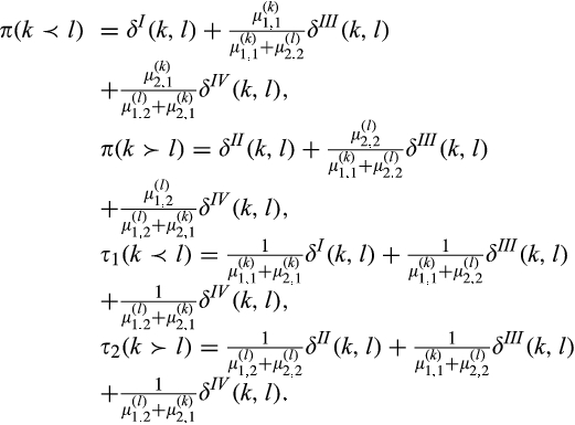
We adopt a methodology similar to Wang et al. (2014). Let T m denote the time point when job m finishes service at station 1. Let R m denote the number of jobs at the buffer and station 2 at time T m . Since the buffer size B = 1, R m can be as large as 2. Let p m,i = Pr{R m = i} denote the probability that job m, upon its service completion at station 1, finds i jobs at the buffer and station 2, for i = 0,1,2. Since job 1, upon its service completion at station 1, always finds the buffer and station 2 empty, we have p 1,0 = 1 and p 1,i = 0, for i = 1,2. The following lemma determines p m,i , for m = 2,…,M.
For m = 2, p
2,0 = π(2 ≻ 1), p
2,1 = π(2 ≺ 1), and p
2,2 = 0. For m = 3,…,M,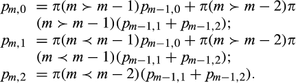
Using the equations in Lemma 1, we can determine all p m,i recursively from m = 1. We calculate the expected makespan using the probabilities p m,i for the rest of this section.
The expected makespan E[D
M
] under a general non‐idling policy can be represented as the sum of the following four components:
Time Durations of Job m = 1,…,M
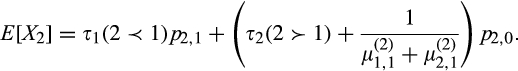
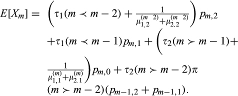
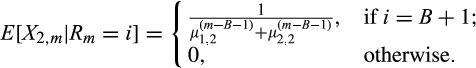
The following proposition determines the expected duration of job m staying at station 1.
For m = 1, For m = 3,…,M,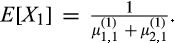
For m = 1, E[W 1] = 0. For m = 2,…,M, the expected duration of job m staying at the initial position equals the sum of the expected durations of job m−1 staying at the initial position and at station 1. That is, E[W m ] = E[W m−1] + E[X m−1]. After obtaining E[X m ], m = 1,…,M, from Proposition 1, we can determine E[W m ] recursively, starting from m = 1.
The following proposition determines the expected duration of job m staying at station 2.
For m = 1,…,M − 2, For m = M − 1, For m = M,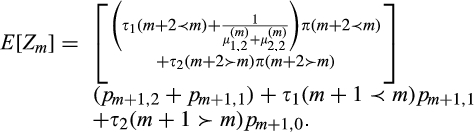

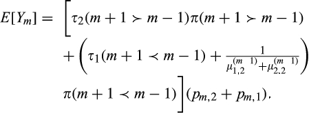
The following proposition determines the expected duration of job m staying at the buffer.
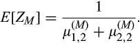
For m = 1, E[Y
1] = 0. For m = 2, For m = 3,…,M − 1, For m = M,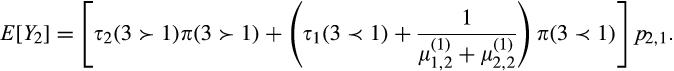
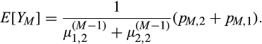
After determining all the four time durations, the expected makespan under a general non‐idling policy can be obtained as E[D M ] = E[W M ] + E[X M ] + E[Y M ] + E[Z M ].
Three Specific Non‐Idling Policies
We analyze three specific non‐idling policies: the summation‐myopic policy, the product‐myopic policy, and the teamwork policy. We derive the expected makespan under each policy using the results in section 4.
If If If If


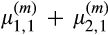
The summation‐myopic policy chooses the assignment that maximizes the sum of the service rates of the two servers for the system's current state. For case I, the maximum rate is 
If If
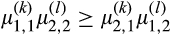
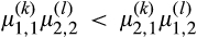
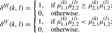
The product‐myopic policy chooses the assignment that maximizes the product of the service rates at the two stations for the system's current state. If the maximum product is 


Using the above indicator functions, we can then obtain π(k ≺ l), π(k ≻ l), τ 1(k ≺ l), τ 2(k ≻ l), and follow the procedure in section 4 to derive the expected makespan E[D M ] under the summation‐myopic policy and the product‐myopic policy.
The teamwork policy is proposed by Van Oyen et al. (2001). It is straightforward to calculate the expected makespan under the teamwork policy without using the indicator functions. That is, 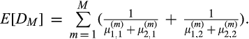
It is worth noting that we do not need the service rates of all the jobs at t = 0 in order to implement the three policies above. Furthermore, although the summation‐myopic policy considers more flexible server assignments than the other two policies, it is not clear whether the former can always outperform the latter policies. We discuss their relative performance in the next section.
Performance Evaluation
We first prove that some of the policies above are optimal for some special cases. For general cases, we compare numerically the performance of these policies against the optimal policy derived from the dynamic program in Table .
Optimality for some Special Cases
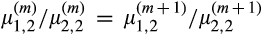
If 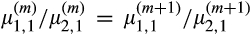
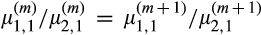
Theorem 1 shows that if the servers maintain the same service‐rate ratio at each station over all the jobs, then the product‐myopic policy is optimal.
If 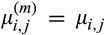
Recall that if the jobs are homogeneous, then the product‐myopic policy is equivalent to the policy in Theorem 4.1 by Andradóttir et al. (2001). In contrast to Theorem 4.1 by Andradóttir et al. (2001) (which studies a system with an infinite number of homogeneous jobs), Corollary 1 shows that the product‐myopic policy is also optimal for minimizing the expected makespan of a system with a finite number of homogeneous jobs.
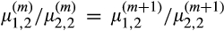
If 
Theorem 2 shows that the teamwork policy is optimal if the servers maintain the same service‐rate ratio at different stations for all jobs n and m, 0 < m − n ≤ B + 1.
The expected makespan of the summation‐myopic policy is no larger than that of the teamwork policy.
It is worth noting that the server assignments under the summation‐myopic policy combine the server assignments under the teamwork policy and the product‐myopic policy. Theorem 3 shows that the summation‐myopic policy is no worse than the teamwork policy. On the other hand, our numerical study in section 6.2 below suggests that the summation‐myopic policy can be better or worse than the product‐myopic policy.
It is straightforward to show that the conditions in Theorem 2: 
If 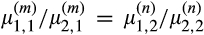
Numerical Study for General Service Rates
We conduct a numerical study to compare the policies for general cases. Figure benchmarks the expected makespan under the summation‐myopic, the product‐myopic, and the teamwork policies against the optimal expected makespan (from the dynamic program in Table ).
Expected Makespan
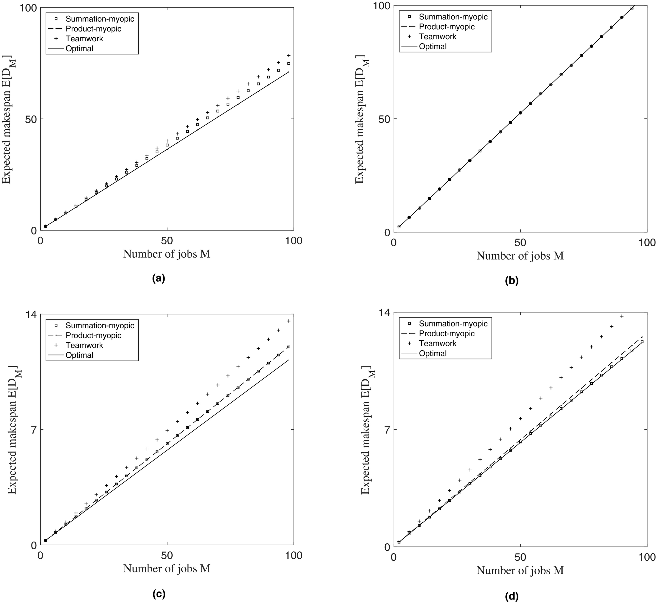
In Figure a, we set 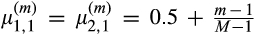


We set 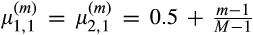


Figure c shows an example where none of the three non‐idling policies is optimal. We set 


Figure d shows another example where none of the three non‐idling policies is optimal. We set 


Among all the parameter settings in Figure , the summation‐myopic policy outperforms the teamwork policy, which is consistent with Theorem 3. However, the summation‐myopic policy can be better (see Figure d) or worse (see Figure a) than the product‐myopic policy. We believe that these different parameter settings cover a wide range of situations that may happen in practice. As shown in Figure , each policy performs differently in different situations.
Extension: General Buffer Size
In this section, we extend the analysis to a system with a general buffer size 
The Optimal Policy
Recall that V(t) denote the number of jobs that are finished at station 1 but not yet finished at station 2 at time t. For a system with a general buffer size B, we have V(t) ∈ {0,…,B + 2}. Note that V(t) = B + 2 if station 1 is blocked at time t. Table describes the dynamic program for the system with a general buffer size B. The expected makespan under the optimal policy is f (M,0).
Dynamic Programming Formulation for a System with a General Buffer Size B
The Expected Makespan of a General Non‐Idling Policy
To derive the expected makespan of a general non‐idling policy, we first calculate p
m,i
, for i = 0,…,m − 1 and m = 1,…,M. Given the buffer size B, we have p
m,i
= 0 for i > B + 1. Since job 1, upon its service completion at station 1, always finds the buffer and station 2 empty, we have p
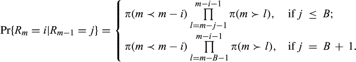
1,0 = 1. The following lemma determines p
m,i
, for m = 2,…,M. For notational convenience, we define π(k ≺ l) = 1 and 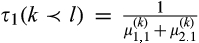
For m = 2,…,M, 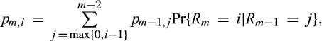
Similar to section 4, to determine the expected makespan E[D M ], we need to derive the four components E[W M ], E[X M ], E[Y M ], and E[Z M ].
We first calculate E[X m ]: the expected duration of job m staying at station 1. We separate the duration of job m staying at station 1, X m , into two parts: the duration of job m staying at station 1 before its service at the station finishes, X 1,m , and the duration of job m staying at station 1 after its service at the station finishes, X 2,m . Note that X 1,m may be longer than the actual service duration of job m at station 1 because job m could be idle at station 1 while both servers work at station 2 (depending on the specific policy used). Furthermore, X 2,m represents the duration when job m is blocked at station 1. Thus, we have E[X m ] = E[X 1,m ] + E[X 2,m ].
To derive E[X
1,m
] and E[X
2,m
], let S
m
denote the number of jobs at the buffer and station 2 found by job m upon entering station 1, for m = 2,…,M. Recall that R
m
denote the number of jobs at the buffer and station 2 found by job m upon its service completion at station 1. Obviously, we have R
m
≤ S
m
. For m = 1, job 1 is first served by both servers at station 1. After that it leaves station 1 without waiting. Thus, we have 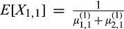
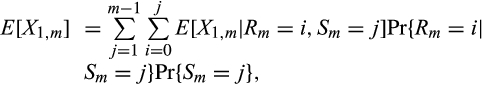


For j = 1,…,B + 1, i = 0,…,j,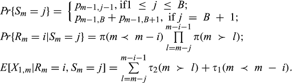
Similar to the case with B = 1, we have E[W 1] = 0 and E[W m ] = E[W m−1] + E[X m−1], for m = 2,…,M. After obtaining E[X m ], m = 1,…,M, from Proposition 4, we can determine E[W m ] recursively, starting from m = 1.
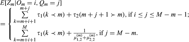
We now calculate E[Z
m
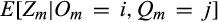
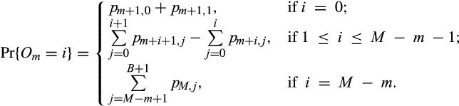
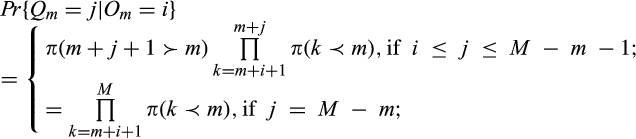
]: the expected duration of job m staying at station 2. Let O
m
denote the number of jobs at the buffer found by job m upon entering station 2, and let Q
m
denote the number of jobs at the buffer and station 2 immediately after job m leaves station 2, for m = 1,…,M − 1. Obviously, we have O
m
≤Q
m
. For m = M, job M is served by both servers at station 2 when it enters the station. Thus, we have 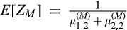
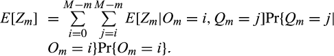

For m = 1,…,M − B,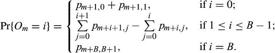
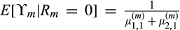
To calculate the duration of job m staying at the buffer, Y m , let Γ m denote the time point when job m enters station 2, for m = 1,…,M. Let ϒ m denote the duration from the time point when job m − 1 leaves station 2 to the time point when job m enters station 2, for m = 2,…,M.
We first derive E[ϒ
m
]. If job m finishes service at station 1 before job m−1 finishes service at station 2 (that is, R
m
> 0), then ϒ
m
= 0. Thus, we have 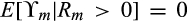

We now derive E[Γ
m
]. For m = 1, 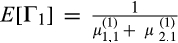
After finding all the four time components, the expected makespan can be obtained as E[D M ] = E[W M ] + E[X M ] + E[Y M ] + E[Z M ].
The Expected Makespans of the Three Specific Non‐Idling Policies
We revisit the three specific non‐idling policies: the summation‐myopic policy, the product‐myopic policy, and the teamwork policy for the system with a general buffer size B. Note that the indicator functions δ I(k,l), δ II(k,l), δ III(k,l), and δ IV(k,l) under the summation‐myopic policy and the product‐myopic policy remain the same as in section 5. Using these indicator functions, we can obtain π(k ≺ l), π(k ≻ l), τ 1(k ≺ l), τ 2(k ≻ l) in section 4, and follow the procedure in section 2 to derive the expected makespan E[D M ] under the summation‐myopic policy or the product‐myopic policy. Note that the expected makespan under the teamwork policy is given in section 5 and is independent of the buffer size.
Performance Evaluation
For the system with a general buffer size B, we have the same results as in section 6 on the optimality of the three non‐idling policies under certain conditions on the service rates.
All the results in Theorems 1‐3 and Corollaries 1‐2 hold for the system with a buffer size 
A numerical study comparing the summation‐myopic, the product‐myopic, and the teamwork policies against the optimal policy (from the dynamic program in Table ) based on general service rates gives very similar results as in Figure . Thus, we do not show the results here.
Extensions: Moving Costs and Service Defects of a General Non‐Idling Policy
Since we characterize the servers’ movements between the stations in our analysis, we can incorporate the costs for the servers to transfer between the stations and the probability of creating defects at each station in the model. In this section, we develop methods to calculate the moving costs and the number of perfect jobs under a general non‐idling policy. We then compare the three specific non‐idling policies in terms of these performance measures. For illustration purposes, we focus on the case with B = 1. To the best of our understanding, moving costs and service defects are generally under studied in the literature. See Andradóttir et al. (2012) for an analysis of a system incurring setup costs when servers move between stations. They consider that the system serves an infinite number of jobs.
Incorporating Moving Costs
Our methodology enables us to calculate the expected total moving cost, which serves as a separate objective besides the expected makespan. We assume that a moving costc 1 (c 2) is incurred every time server 1 (server 2) moves from one station to another. Suppose servers 1 and 2 are currently at stations s 1 and s 2, respectively, where s 1,s 2 = 1,2. If we choose server assignment I in section 3, then a moving cost c I(s 1,s 2) = (s 1 − 1)c 1 + (s 2 − 1)c 2 is incurred. Similarly, we have c II(s 1,s 2) = (2 − s 1)c 1 + (2 − s 2)c 2, c III(s 1,s 2) = (s 1−1)c 1 + (2 − s 2)c 2, and c IV(s 1,s 2) = (2 − s 1)c 1 + (s 2−1)c 2, for server assignments II, III, and IV, respectively.
Suppose in the current state, neither station 1 is blocked nor station 2 is starved, jobs k and l are at stations 1 and 2 respectively, and servers 1 and 2 are at stations s 1 and s 2, respectively. For a system with M jobs, let C (M)(k,l,s 1,s 2) denote the expected moving cost from the current state until the completion of all the jobs under a general non‐idling policy. For notational convenience, let k = 0 represent the case when station 1 is blocked or job M has finished its service at station 1, and let l = 0 represent the case when station 2 is starved.
Suppose in the current state, station 1 is not blocked, job M has not finished its service at station 1, and station 2 is not starved. Assume jobs k and l are at stations 1 and 2 respectively, and servers 1 and 2 are at stations s 1 and s 2 respectively. For a system with M jobs, let C (M)(k,l,s 1,s 2) denote the expected moving cost from the current state until the completion of all the jobs under a general non‐idling policy. For a state in which station 1 is blocked or job M has finished its service at station 1, let C (M)(0,l,s 1,s 2) denote the expected moving cost from the state until the completion of all the jobs under a general non‐idling policy. Similarly, for a state in which station 2 is starved, let C (M)(k,0,s 1,s 2) denote the expected moving cost from the state until the completion of all the jobs under a general non‐idling policy.
Let 
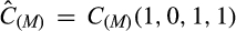
Figure compares the expected total moving costs of the three policies. We set c 1 = c 2 = 1. For each sub‐figure of Figure , we use the same parameter setting as in the corresponding sub‐figure of Figure . Figure a shows that the teamwork policy leads to the largest expected total moving cost, followed by the summation‐myopic policy. The product‐myopic policy has the smallest expected total moving cost. The rankings of the policies are identical to that of Figure a, which is based on the expected makespan. It is interesting to compare Figures b and b. Although the three policies lead to the same expected makespan, they produce very different expected total moving costs. Comparing Figures c and c suggests that the summation‐myopic and the product‐myopic policies yield not only the same expected makespan, but also the same expected total moving cost. This suggests that the two policies are identical under this parameter setting. In contrast to Figures a–d shows that the summation‐myopic policy may lead to a smaller expected total moving cost than the product‐myopic policy.
Expected Total Moving Cost
Incorporating Service Defects
We now consider a system that may generate defects. We assume two types of service defects: Type‐1 (type‐2) defects only occur at station 1 (station 2). These two types of defects occur independently. For each job, the probability of having a type‐j defect depends on who serves the job at station j, j = 1,2. This probability is determined by one of the following scenarios: The job is finished only by server i at station j (this includes the case in which the job is first served by another server i
′ and later finished by server i at that station). The probability for the job to have a type‐j defect is d
i,j
. The job is finished by both servers at station j (this includes the case in which the job is first served only by one server and later finished by both servers at that station). The probability for the job to have a type‐j defect is d
j
.
Define 
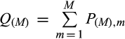
If M = 1, then 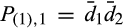
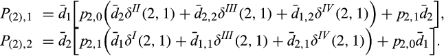
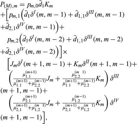
To calculate P
(M),m
and Q
(M) for the summation‐myopic policy or the product‐myopic policy, we can substitute the corresponding indicator functions δ
I(k,l), δ
II(k,l), δ
III(k,l), and δ
IV(k,l) from section 5 into Proposition 6. It is straightforward to see that under the teamwork policy, we have 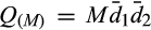
We conduct a numerical study to compare the three policies in terms of the expected number of perfect jobs. We consider the following three cases:
d
1 < d
i,1,d
2 < d
i,2. d
1,1 < d
1,2,d
2,2 < d
2,1.
d
1 > d
i,1,d
2 > d
i,2. d
1,1 < d
1,2,d
2,2 < d
2,1.
d
1 < d
i,1,d
2 > d
i,2. d
1,1 = d
2,1,d
1,2 = d
2,2.
Figure a shows the expected percentage of perfect jobs under each policy for case (i). We use the same parameter setting as in Figure a. We set d 1 = d 2 = 0.02, d 1,1 = d 2,2 = 0.1, and d 1,2 = d 2,1 = 0.2. Since d j < d i,j , for i,j = 1,2, the teamwork policy yields the largest expected percentage of perfect jobs in Figure a as the servers always work jointly under this policy. The performance of the summation‐myopic policy falls in the middle, producing a larger expected percentage of perfect jobs than the product‐myopic policy. This is because under the product‐myopic policy, the two servers generally work separately (unless the system is blocked or starved), which leads to more defects. In contrast, the summation‐myopic policy mixes the server assignments of the other two policies, producing the expected percentage of perfect jobs that always falls between that of the two policies.
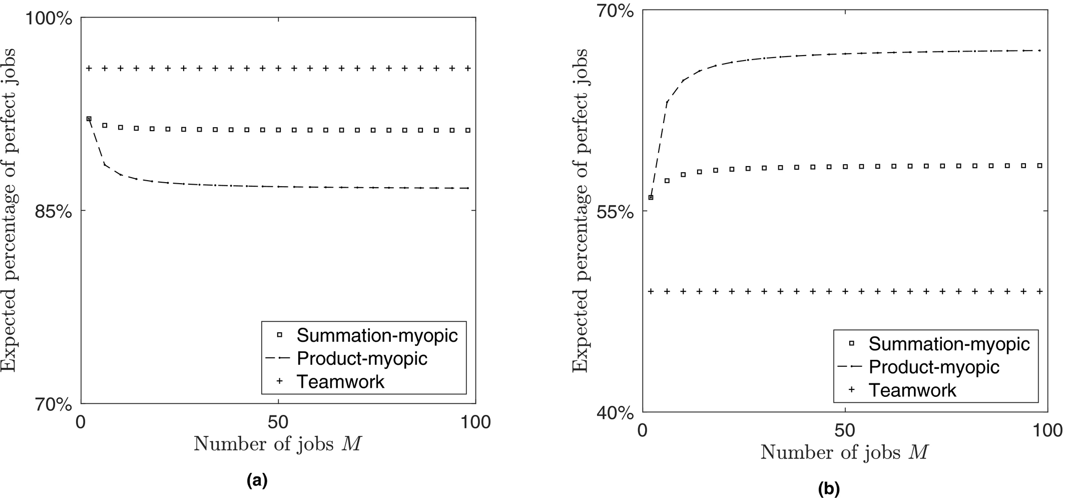
Expected Percentage of Perfect Jobs
Using the same parameter setting as in Figures a and b shows the expected percentage of perfect jobs under each policy for case (ii). We set d 1 = d 2 = 0.3, d 1,1 = d 2,2 = 0.1, and d 1,2 = d 2,1 = 0.2. In this case, we have d j > d i,j , for i,j = 1,2. In contrast to case (i), the teamwork policy yields the smallest expected percentage of perfect jobs in this situation. The performance of the summation‐myopic policy remains in the middle, and the product‐myopic policy gives the largest expected percentage of perfect jobs.
Figure shows the expected percentage of perfect jobs under each policy for case (iii). In this case, the servers are less likely to create defects when they work jointly at station 1, but are more likely to create defects when they work jointly at station 2. For each sub‐figure of Figure , we use the same parameter setting as in the corresponding sub‐figure of Figure . We set d 1 = d 2 = 0.1, d 1,1 = d 2,1 = 0.2, and d 1,2 = d 2,2 = 0.02. The teamwork policy yields the same expected percentage of perfect jobs in all the sub‐figures. Figure a shows that the product‐myopic policy outperforms the summation‐myopic policy, whereas we have the opposite result in Figure d. Both policies produce fewer defects than the teamwork policy. In Figure c, the summation‐myopic policy produces the same expected percentage of perfect jobs as the teamwork policy, whereas the product‐myopic policy creates the largest number of defects. Figure shows that the summation‐myopic and the product‐myopic policies produce the same expected percentage of perfect jobs. This again verifies that these two policies are identical under this parameter setting.
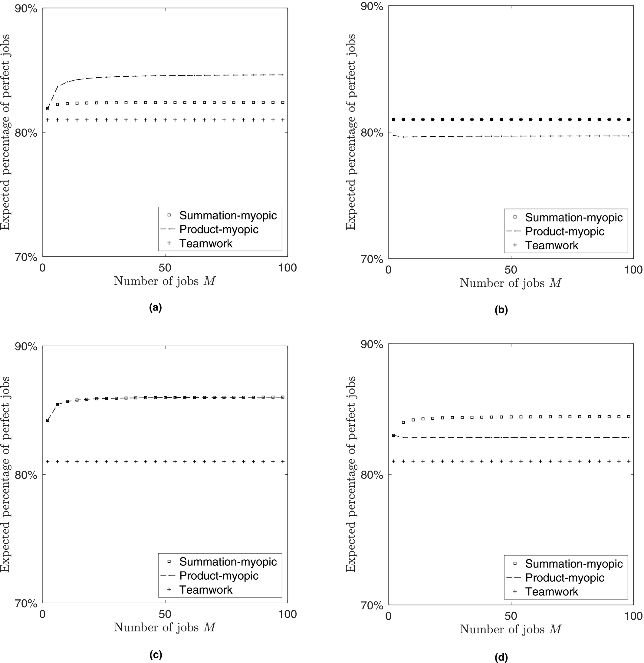
Expected Percentage of Perfect Jobs
Conclusion
We study a two‐station, two‐server tandem system serving a finite number of jobs. There is a finite buffer between the stations. The servers are cross‐trained such that they can work at both stations. The duration for each server to serve a job at each station is exponentially distributed with a rate that depends on the server, the station, and the job. This tandem system is common in the manufacturing and the service industries, where workforce is a major operating cost. In these environments, it is important to maximize the productivity by effectively using the workforce.
We formulate a stochastic dynamic program to identify an optimal policy that dynamically assigns the servers to the stations to minimize the expected makespan. Unfortunately, the optimal policy is too complicated to characterize for a large number of jobs. This motivates us to develop simpler and more intuitive policies. We use the optimal policy as a benchmark when we evaluate the simpler policies.
Since the optimal policy is non‐idling, we focus on non‐idling policies in this study. Using the basic probability theory, we first derive the expected makespan of a system with a buffer size B = 1 under a general non‐idling policy. We then analyze three specific non‐idling policies: the summation‐myopic, the product‐myopic, and the teamwork policies. We prove that the product‐myopic policy is optimal in minimizing the expected makespan if the servers maintain the same service‐rate ratio at each station for all the jobs (see Theorem 1). Furthermore, if the service rates are independent of the jobs (that is, the jobs are homogeneous), then the product‐myopic policy is optimal (see Corollary 1). We also prove that the teamwork policy is optimal if the servers maintain the same service‐rate ratio at different stations for all jobs n and m, 0 < m − n ≤ B + 1 (see Theorem 2). Finally, we prove that the expected makespan of the summation‐myopic policy is no larger than that of the teamwork policy (see Theorem 3). On the other hand, our numerical study based on general service rates suggests that the summation‐myopic policy can be better or worse than the product‐myopic policy.
We extend the analysis to a system with a general buffer size 
Footnotes
Acknowledgment
The authors thank the senior editor and the two anonymous referees for their valuable comments that have substantially improved the paper. The first author is grateful for the support from the Singapore Management University under the Lee Kong Chian Fellowship and the Ministry of Education, Singapore under the MOE Tier 1 Academic Research Fund.