
Abstract
We propose a model to assess the value of a distributor in a dynamic stochastic cooperative advertising supply chain in which a manufacturer wholesales its product to a distributor who in turn sells it to a retailer. Moreover and importantly, the distributor also intermediates the pricing and advertising decisions between the manufacturer and the retailer. For the resulting three‐player hierarchical game formulation of the supply chain, we characterize the feedback Stackelberg equilibrium in terms of a system of coupled algebraic equations and show it to admit a unique solution. We find that the value added by the distributor to the supply chain depends critically on the nature of the demand function for the product, a result that has practical implications for the kinds of product where having a distributor is most desirable. Second, our model indicates that the presence of the distributor can enhance the margins of both the retailer and the manufacturer relative to the case of no distributor, and provide explicit conditions for this to occur. Third, we present numerical analysis that indicates that if the distributor generates sufficiently large transportation cost savings, then the three‐echelon supply chain can lead in the long run to higher market awareness, lower advertising expenditure, and higher value extracted, relative to the two‐echelon model. Finally, in addition to retailer advertising that is subsidized by the manufacturer, we also provide the manufacturer an option to do national advertising and show its viability.
Keywords
Introduction
Cooperative (co‐op) advertising programs are common in supply chains as a means of boosting market share and influencing retailer behavior. As an increase in the market share of a product benefits every member of the supply chain, they have a common interest in promoting the product. Furthermore, as co‐op advertising makes up a significant portion of total advertising expenditure (Dant and Berger 1996), there is a clear monetary benefit to studying them and deriving the optimal strategies of the players involved. For this reason, many prominent models have been proposed to quantify the effects of advertising on sales in a supply chain. For the comprehensive coverage of the early representative models, readers are referred to Sethi (1977), Erickson (1995), Feichtinger et al. (1995), and the references therein.
One prominent model used for sales‐advertising dynamics is the Sethi advertising model first proposed by Sethi (1983). Previously, advertising and sales were generally modeled deterministically, without concern for random effects due to external factors. Sethi (1983) introduced a tractable advertising model that included a random noise process to represent all random effects out of the control of the advertising firm. The continuous‐time framework of Sethi (1983) also allows us to analyze the stationary distribution of the firm's sales under the optimal strategy in feedback form.
Based on the Sethi model, He et al. (2009) studied a two‐player stochastic differential game comprising of both optimal pricing and co‐op advertising. They formulated the problem as a stochastic Stackelberg differential game with a clear “leader‐follower” hierarchy, in which the manufacturer enjoys the first‐mover advantage at each time instant, in contrast to a Nash game in which both players act at the same time. The game proceeds as follows: The manufacturer first announces a subsidy percentage of the final advertising expenditure, after which the retailer decides its advertising effort. He et al. (2009) managed to obtain a condition determining when the provision of an advertising subsidy is optimal to the manufacturer. In addition, they found that the commonly used linear and isoelastic demand functions give rise to cases with and without advertising subsidy, respectively. They also compared the optimal advertising and pricing decisions derived under the co‐op model against those of a single integrated supply chain. In particular, they highlighted that, all else being equal, the value function of the integrated supply chain is higher than the sum of the value functions of the manufacturer and the retailer in the decentralized supply chain, owing to the problem of double marginalization. Finally, they showed that a revenue‐sharing contract together with a co‐op advertising program can coordinate the marketing channel.
In practice, it is common for a distributor to act as a middleman between a retailer and a manufacturer, particularly for multinational companies that sell products in multiple markets. Since they sell to retailers in many regional markets, it is more difficult for the manufacturer to tailor its behavior to accommodate retailers in a single region. In contrast, the distributor, who specializes in serving retailers in a single region, can form a closer relationship with the retailer than the manufacturer can, owing to the distributor's geographic proximity, and therefore improves the transportation efficiency of the supply chain. Here, transportation efficiency refers to how efficient the supply chain is, in terms of time and cost, in transporting goods. Indeed, as discussed in Bradley (1998) and Cooke (1998), distributors typically serve as third‐party logistic providers to manufacturers in terms of providing warehousing, transportation services, as well as specialized informational technology that would be too expensive for the manufacturers to provide alone. A natural extension of previous work is therefore to introduce a middleman that plays the role of a distributor. In exchange for taking a cut of the total profit margin, this additional player should improve the transportation efficiency of the supply chain in some sense. Furthermore, the distributor might also contribute to the supply chain's promotional efforts by promoting the product to additional retailers, thus boosting the product's exposure.
We, therefore, extend the earlier co‐op advertising models to include a distributor, or a wholesaler, as a three‐player Stackelberg stochastic game. In particular, we extend the model introduced by He et al. (2009) by incorporating both the optimal pricing and co‐op advertising problems into the model, with the distributor acting as an intermediary between the manufacturer and the retailer. Essentially, the distributor acts as a decoupling point between the manufacturer and the retailer to alleviate the differing business models and the risks associated with them. For example, the manufacturer deals in large volume orders, while the retailer prefers low volume orders due to limited storage space. By acting as an intermediary between the two, the distributor can arrange the desired order sizes for each of them. In addition, we allow the manufacturer to engage in a national advertising campaign alongside its co‐op advertising program with the retailer. Moreover, we suppose that the distributor can also conduct an advertising effort independent of the other players, with distinct advertising effectiveness, representing all promotional activities carried out by the distributor. The question we seek to answer is whether the efficiency gained through the addition of the distributor is enough to justify the distributor's presence in the supply chain. Indeed, the inclusion of the distributor will clearly lead to an additional marginalization relative to the benchmark two‐echelon model. Notwithstanding, we show that the transportation efficiency gained from the distributor's presence can offset the additional marginalization.
In the optimal pricing problem, each player must set the price at which they are willing to sell the product. The manufacturer first announces the manufacturer's wholesale price, followed by the distributor who announces the distributor's wholesale price and finally the retailer who announces the retail price. The optimal pricing problem depends critically on the chosen demand function, which represents consumer demand of the product from the retailer. In this study, we consider both linear and isoelastic demand functions, and derive the resulting optimal prices. We are able to obtain closed‐form expressions for the optimal prices for both demand functions considered. We then study how the players’ prices and margins are affected by transport costs, as well as the effect of the distributor's presence. Interestingly, we find that the optimal behavior varies quite considerably in some respects between the linear and isoelastic demand functions.
For the co‐op advertising problem, we assume local and national advertising efforts are undertaken separately, while the local advertising effort is subsidized. As is standard in the existing literature, the manufacturer subsidizes the retailer's local advertising effort via a vertical co‐op advertising program, while simultaneously engaging in its own national advertising effort. In addition, we allow the distributor to engage in its own promotional activities, with distinct advertising effectiveness, independent of both the local and national advertising efforts. Therefore, the manufacturer acts first by announcing its wholesale price to the distributor, national advertising effort, and co‐op participation rate. Following this, the distributor announces its wholesale price to the retailer and its own advertising effort representing all promotional activities undertaken by the distributor. Finally, given the manufacturer's and distributor's policies, the retailer announces its local advertising effort and the retail price. With linear value functions for the players in an equilibrium solution, we derive a system of coupled equations for the value function parameters. We are able to show that a unique solution exists under mild conditions on the players’ margins.
On the theoretical level, this study contributes to the existing literature on stochastic Stackelberg advertising models by providing a complete analysis on the establishment of the feedback Stackelberg solution. First, we employ the dynamic programming principle to show that the hierarchical structure of the decision‐making in the three‐echelon model can be reduced to solving the nested Hamiltonian systems among the three players at each time instant. Second, our problem formulation allows us to further characterize the solutions of the nested Hamiltonian systems in terms of the solutions of systems of coupled algebraic equations. In addition, we prove that the system of coupled algebraic equations admits a unique solution triplet. Finally, we apply the verification theorem in the sense of Bensoussan et al. (2019) to verify that our solution triplet indeed provides an optimal feedback Stackelberg equilibrium among three players.
From the modeling perspective, we provide detailed analytical and numerical analyses on quantifying the savings due to the transportation efficiency brought about by the distributor. Under the linear and isoelastic demand functions, we provide explicit expressions for how much transportation cost savings the distributor must generate in order to benefit the other players, as well as consumers via a reduced retail price. The advertising decisions are comparatively more difficult to obtain analytically, and so we instead identify several metrics to numerically illustrate the benefit of bringing in the distributor in the context of advertising. In other words, our results suggest that the problem of the additional marginalization can also be circumvented from the perspective of the distributor's presence generating transportation cost savings.
To our knowledge, there is little in the literature that studies the value of a distributor, a wholesaler, or a middleman more generally, in dynamic supply chain settings. Given the important role the distributors play in an increasingly globalized world, there is a clear motivation for understanding the value they offer and, more specifically, what products benefit the most from the presence of the distributor. In this study, we introduce them into a co‐op advertising framework as a first step, with the hope of expanding this research area in future works.
The structure of this study is as follows. In section 2, we review recent work on supply chain and stochastic advertising games. In section 3, we introduce the model as a three‐player stochastic differential game as well as an additional two‐player game that serves as a benchmark. In section 4, we present important analysis including an existence and uniqueness result. Finally, in section 5 we present and discuss numerical results. Proofs of the results presented can be found in the online appendix.
Background Literature
This study combines work on product pricing within operations management with recent literature on co‐op advertising, studied within the framework of a stochastic differential game. It further seeks to expand the existing literature to a more relevant setting through the addition of a distributor, or equivalently, a wholesaler.
Although little attention has been paid to the presence of distributors within dynamic supply chains or marketing channel models, much research has been done within an empirical or a static modeling framework to study the gains in efficiency that they provide. Balakrishnan et al. (2000) derived an optimal delivery fee scheme in a static framework that generated considerable economic savings for the manufacturer and provided more equitable compensation to downstream distributors. Chopra (2003) discussed how the value added by the distributor stems primarily from a reduction in inbound and outbound transportation costs, a reduced inventory cost, a more stable order stream from the distributor to the manufacturer allowing for more effective production planning, and storing product close to the point of sale. Chung and Ng (2008) studied the role of distributors in supply chains and explored the positive contributions they offer. They explained how the distributor serves as a decoupling point by taking on risk from both upstream and downstream parties. They took on both the overstock risk from the upstream parties that deal in economies of scale, while simultaneously providing fast delivery on low quantity orders to downstream parties. Zou et al. (2011) studied the problem of distributor evaluation and selection using a rough set‐based approach, identifying marketing experience, management ability, and relationship intensity as the most important factors. Recent literature has also considered the role of a supplier in some three‐echelon models. For example, Huang and Wang (2017) studied the value of information flow in a three‐echelon model in which the supplier sells the components to the manufacturer, who in turn sells the finished products to the retailers. Taleizadeh and Moshtagh (2018) studied a consignment stock scheme with lost sales effect and quality‐dependent returns in a closed‐looped multi‐echelon model in which the supplier serves as the Stackelberg leader. Both of the aforementioned works based their models in a static and deterministic framework, suggesting that the exploration into the multi‐echelon models has just begun.
Dynamic co‐op advertising has received much attention in recent years. Jørgensen et al. (2000) considered an interesting model consisting of a manufacturer and an exclusive retailer in which the players have both short‐ and long‐term advertising efforts, and the manufacturer also subsidizes the retailer's advertising efforts. Jørgensen et al. (2001, 2003) studied models in which the manufacturer and the retailer run national and local advertising campaigns, respectively, where the manufacturer contributes to accumulated goodwill. They characterized stationary feedback equilibria for both with and without the manufacturer's support for the retailer's local advertising effort. He et al. (2009) combined the co‐op advertising problem with that of product pricing in a stochastic differential game setting. They compared the decentralized model with the centralized one, and found that the decentralized channel results in higher than optimal prices with lower than optimal advertising. Sigué and Chintagunta (2009) studied advertising within a franchise system, studying a two‐stage advertising game consisting of a franchiser and two adjacent franchisees, exploring the conditions under which franchisees should cooperate. Zhang et al. (2013) extended the co‐op advertising framework to include a reference price. They assumed that advertising has a positive effect on a customer's reference price and goodwill, which in turn has a positive effect on sales. Recently, Lu et al. (2019) studied a manufacturer–retailer supply chain with co‐op advertising in which the product experiences price stickiness, where each player may be either myopic or farsighted. They found that a low degree of price stickiness, combined with a co‐op advertising subsidy, can help the players escape from the prisoner's dilemma. For comprehensive reviews of game‐theoretic static and dynamic models for co‐op advertising and pricing, readers are referred to Huang et al. (2012), Jørgensen and Zaccour (2014), Aust (2014), Li and Sethi (2017), and Giovanni and Zaccour (2019). In particular, Li and Sethi (2017) have pointed out that Stackelberg games have been particularly useful in studying inventory issues, wholesale and retail pricing strategies, and outsourcing. Giovanni and Zaccour (2019) gave a survey of general closed‐loop models for general supply chains considering return functions and coordination mechanisms, such as co‐op advertising. They highlighted that the current coordination literature (see e.g., Cachon 2003) has focused primarily on cost and revenue‐sharing contracts, and suggests various types of contracts and competition as areas of further research.
An extension to the traditional manufacturer–retailer co‐op advertising supply chain was proposed in Chutani and Sethi (2018), in which multiple manufacturers sell their products independently through multiple retailers. In a similar vein, He et al. (2012) considered a co‐operative advertising Stackelberg game where a manufacturer sells a product via a retailer, with a Nash sub‐game in which the retailer competes with an additional external retailer. Prasad et al. (2012) took this idea further by introducing the effect of churn, the turnover rate at which customers switch to competing brands, to a dynamic advertising model. Pan et al. (2009) considered the interesting case where a retailer channel is dominated by a single dominant retailer, such as Walmart, who can leverage the dominant position to dictate prices and ordering policies. They studied the optimal pricing and ordering policies of the dominant retailer within a two‐period model with demand uncertainty and a deteriorating price environment. Huang et al. (2011) used a game‐theoretic approach to studying inventory and pricing coordination and component selection within a multi‐level supply chain consisting of multiple retailers and suppliers, with a single manufacturer, assuming linear demand. In contrast to these works, this study considers only a single player at each level, however, introducing competition among players at each level presents an area of further research, and the current paper serves as a stepping stone in that direction.
The Model and Problem Formulation
We consider a supply chain where the manufacturer sells its product to the retailer via the distributor. Associated with the supply chain is the market awareness X t of the product which determines the total sales. The retailer decides the retail price P R and sets the local advertising effort α R with advertising effectiveness ψ R . The distributor decides the distributor price P D and sets the distributor's advertising effort α D , representing all promotional activities carried out by the distributor, such as promotional activities carried out by its salesforce, with advertising effectiveness ψ D . Finally, the manufacturer decides a wholesale price P M , a national advertising effort α M with a given advertising effectiveness ψ M , and a subsidy rate ϕ to the retailer's local advertising effort through a vertical co‐op advertising program.
Following He et al. (2009), the advertising expenditure is quadratic in effort. That is, the total advertising costs are given by


To model the combined effect of each player's advertising effort, we use an extension of the Sethi advertising model. This is defined by the stochastic differential equation


The state equation is specified to reflect our intuitive understanding of sales‐advertising dynamics, as well as for mathematical convenience. First, the market awareness increases with advertising effort with diminishing returns as awareness reaches saturation, and also includes a decay to represent all external factors that drive market awareness down. Second, by using distinct effectiveness parameters ψ R , ψ D , and ψ M we can incorporate the idea that local and national advertising campaigns may differ in their impact. In particular, we can set ψ R > ψ M to model the fact that local advertising campaigns are more localized, and hence are generally more impactful. Finally, we require the manufacturer's subsidy or participation rate ϕ(t) in the co‐op problem to be in [0, 1]. Although ϕ(t) does not directly appear in the state equation, we will see later that it appears in the objective functions of the manufacturer and the retailer, and therefore, the retailer's optimal advertising effort does depend on the state. Hence, the state equation depends on the manufacturer's subsidy rate via the retailer's optimal advertising effort.
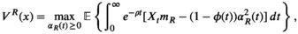
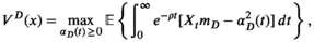
We model the supply chain problem as a Stackelberg stochastic differential game over an infinite time horizon with a discount rate ρ > 0. In addition, we restrict our attention to finding the feedback Stackelberg solutions in which the optimal strategies of the players, that is, the retailer, the distributor, and the manufacturer, depend on the current state X t and time t. We refer the reader to Bensoussan et al. (2015b) for the rigorous definition of the feedback Stackelberg strategies in continuous time. Since we consider the Stackelberg stochastic differential game over an infinite time horizon, the optimal strategies of the players will be given in terms of the current state X t . Specifically, the manufacturer, anticipating the distributor and retailer responses, enjoys the instantaneous first‐mover advantage by first announcing the wholesale price P M (t), the national advertising effort α M (t), and the co‐op participation rate ϕ(t). This is followed by the distributor who, anticipating the retailer's response, then announces the distributor price P D (t) and the distributor advertising effort α D (t). Finally, the retailer then announces the retail price P R (t) and local advertising effort α R (t). Although the players’ optimal strategies are expressed in terms of X t , we nevertheless will continue to write them as functions of t throughout this study for notational convenience.
Different from He et al. (2009), we allow the manufacturer to engage in a national advertising campaign, in addition to providing a co‐op subsidy to the retailer's local advertising effort. To the best of our knowledge, the consideration of national advertising in the context of a co‐op local advertising program has not been well studied under the Sethi (1983) model. Indeed, Aravindakshan et al. (2012) solved an optimal local and national advertising problem of a single firm under a spatiotemporal allocation model, which can be seen as a variant of the Sethi (1983) model. Jørgensen et al. (2000, 2003) have studied the inclusion of national advertising in a co‐op advertising program under the Nerlove‐Arrow (1962) model, where the optimal controls of the manufacturer and the retailer are independent of the market awareness. However, the impact of national advertising in a dynamic co‐op advertising problem under the Sethi model is more complicated, since the optimal controls of the players, that is, advertising efforts and subsidy decisions, are expressed in terms of market awareness. Indeed, Bensoussan et al. (2019) had initiated a co‐op advertising problem with national advertising in a mixed leadership model. However, the complexity of their model only allowed them to study the subsidy decision numerically. In contrast, in section 4, we will solve analytically not only the three‐echelon model given above, but also the two‐echelon manufacturer–retailer model with both national advertising and co‐op subsidy, thereby also extending the earlier work of He et al. (2009).
We also introduce transport costs to the distributor and the manufacturer to model the costs associated with the transportation of product. We define a player's transport cost as being proportional to demand, with transport cost parameters k D and k M . It is assumed that the retailer incurs no transport cost, while k D and k M reflect the difference in transport cost between the distributor and the manufacturer due to distance and volume. This formulation of transport cost captures the realistic situation in which the manufacturer produces its product in a region where production is most efficient, ships it to the distributor located in a region that is good for business, who in turn ships the product to the retailer for sale to consumers.
The manufacturer's, the distributor's, and the retailer's optimal control problems are given respectively as follows:


The demand function D(P R ) should be downward sloping and differentiable to reflect the realities of price dynamics. In this study, we specifically consider the linear and isoelastic demand functions for illustration, the same demand functions considered in He et al. (2009) who point out that they are the most commonly used demand functions. Furthermore, these demand functions admit closed‐form solutions for the optimal prices. For an in‐depth discussion on linear and isoelastic demand functions, we refer the reader to Petruzzi and Dada (1999). In He et al. (2009), it is seen that the linear and isoelastic demand functions generate opposite implications on whether or not advertising subsidy by the manufacturer is optimal. Indeed, we will see later that the two demand functions can similarly lead to different optimal strategies under our three‐echelon model.
The linear demand function is defined as


To highlight the transportation efficiency achieved by the distributor, we also define a two‐echelon model to serve as a benchmark. In this two‐echelon model, the manufacturer sells directly to the retailer, without the distributor serving as a middleman, while simultaneously engaging in both a national advertising campaign and a co‐op advertising program with the retailer. This simpler two‐echelon model is an extension of that considered in He et al. (2009) in that the manufacturer also runs a national advertising campaign. Furthermore, the transport costs must now be paid solely by the manufacturer. This set up is chosen as a benchmark for the centralized supply chain, as is normally considered in the related literature, to highlight the intermediary role of the distributor as a decoupling point between upstream and downstream members of the supply chain. Specifically, we exclusively seek to investigate when the presence of an intermediary is beneficial, rather than comparing our three‐echelon supply chain with the centralized supply chain.
The two‐echelon model is, therefore, defined by


When comparing the two‐ and three‐echelon models, we introduce a parameter ξ that represents all transport cost savings owing to the presence of the distributor. It is thus assumed that
The above co‐op advertising model can also be reformulated as a co‐op selling model, where the players’ controls are the number of employed salespersons instead of their advertising efforts. See Online Appendix A for details.
Solution
In this section, we will derive the optimal pricing and advertising strategies for each of the players in the two‐ and three‐echelon models presented in section 3. Despite the complexity of the three‐echelon model, we manage to obtain a closed‐form feedback solution to the associated Stackelberg equilibrium and show that the value functions of the manufacturer, the distributor, and the retailer are linear. We begin by considering the three‐echelon model since corresponding results for the two‐echelon sub‐model are comparatively simpler.
Three‐Echelon Form
We divide our analysis into two parts. The first part involves optimal pricing, while the second part involves optimal advertising strategies. The first key observation is that the pricing and advertising problems for each player of the supply chain can be solved separately. This is because the prices P R , P D , and P M do not appear in the state equation of X t in Equation (1). The integrals can therefore first be maximized with respect to these prices, and then the corresponding advertising controls using the dynamic programming approach.
Optimal Pricing
By the hierarchical nature of our Stackelberg game, we begin by deriving the retailer's optimal price which will be a function of the distributor's. This is then substituted into the distributor's integral so that the distributor's optimal price can be derived. Finally, the optimal retailer and distributor prices are substituted into the manufacturer's integral, and the manufacturer's optimal price is obtained.
For the three‐echelon model with the linear demand function defined by Equation (5), the optimal prices are given by

For the three‐echelon model with the isoelastic demand function defined by Equation (6), the optimal prices are given by

Propositions 1 and 2 highlight that an important difference between the linear and isoelastic demand functions is how the manufacturer's optimal price


Optimal Advertising Strategies
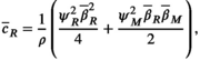
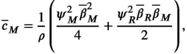
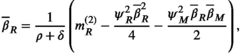
To ease notation, we now define the following quantities involving the optimal prices:


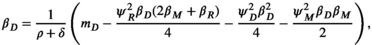
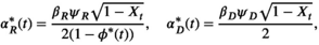
To find the Stackelberg equilibrium, we begin by deriving the retailer's optimal advertising effort


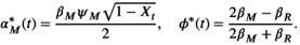
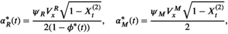
The optimal strategies in the three‐echelon model are given by
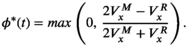
Proposition 3 shows that the optimal advertising effort

In the case ϕ*(t) = 0, the value functions V
R
(x), V
D
(x), V
M
(x) are linear in x, as follows:


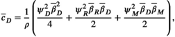
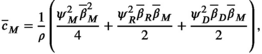
For the value functions in Proposition 4 to be the solution of the three‐echelon problem with no subsidy, we need to ensure that


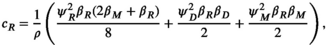
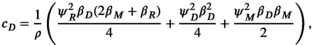
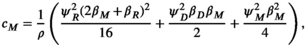
With linear value functions, Proposition 5 establishes that a unique positive solution


Next, we proceed to tackle the existence and uniqueness of the solution for the general case ϕ*(t) ≠ 0, in which the manufacturer does subsidize the retailer's local advertising campaign.
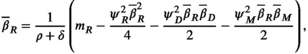
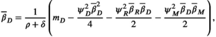
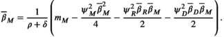
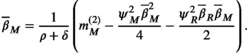
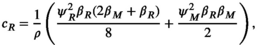
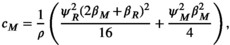
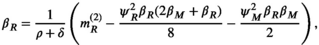
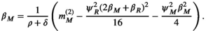
In the case ϕ*(t) ≠ 0, the value functions V
R
(x), V
D
(x), V
M
(x) are linear in x, as follows:


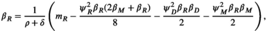
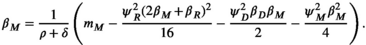
As in the case of no subsidy, we need to ensure that


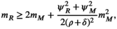
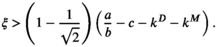
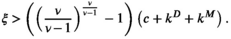
Suppose the retailer and manufacturer margins satisfy

The condition (30) is natural within the context of a vertical co‐op local advertising program; the manufacturer will only be incentivized to subsidize the retailer's advertising expenditure if its margin is sufficiently large relative to that of the retailer. If the condition is not satisfied, so that the retailer makes the majority of the profit, it makes little sense for the manufacturer to provide a subsidy. Indeed, we will see that the quantity on the left‐hand side of Equation (30) frequently appears in subsequent results.
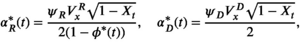
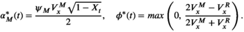
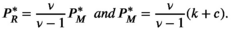
With linear value functions, Proposition 7 establishes that the corresponding Stackelberg equilibrium strategies of all three players are
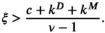
With the Stackelberg equilibrium strategies established for the subsidy and no‐subsidy cases, it remains to identify the situations under which a subsidy from the manufacturer will be provided. When there is no distributor and no national advertising, He et al. (2009) derived explicitly a necessary and sufficient condition for the manufacturer to subsidize the retailer, thanks to the key observation that the resulting equations under the no‐subsidy case are not coupled. However, as shown in Equations (21)–(23) and (27)–(29), the presence of national advertising leads to the equations remaining highly coupled in both cases, and this significantly increases the difficulty of finding a necessary and sufficient condition for the provision of subsidy. Nonetheless, the following proposition provides necessary and sufficient conditions depending only on the model parameters.
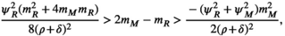
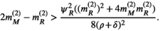
A sufficient condition for the manufacturer to subsidize the retailer is
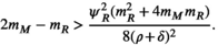
According to Proposition 8, the manufacturer will provide subsidy to the retailer's local advertising effort when its margin m
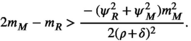
M
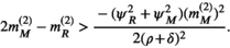
satisfies the sufficient condition in Equation (33). On the other hand, the necessary condition (34) indicates that when the manufacturer's margin is too low relative to that of the retailer, that is,

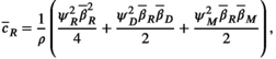
We conclude this section by establishing that the long‐run market awareness follows a Beta distribution in the three‐echelon model. It is useful to derive the long‐run mean of the market awareness as it allows us to study the general long‐run behavior of the players under the feedback equilibrium strategies, and provides us with a useful tool for model comparison in section 5.
Suppose that

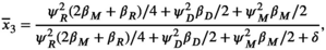

Since


Two‐Echelon Form
As the two‐echelon model is simply a sub‐model of the three‐echelon model, similar results can be given which we present in this section. We proceed with the leader–follower set up as in the previous section, with the only significant difference being the exclusion of the distributor and its associated controls. To avoid overburdening the paper with notations, we use the same set of notations as in section 4.1 unless stated otherwise.
Optimal Pricing
As the two‐echelon pricing problem can be seen as a sub‐problem of the three‐echelon pricing problem, the optimal prices are immediate, and hence their proofs are omitted.
For the two‐echelon model with the linear demand function, the optimal prices are given by

For the two‐echelon model with the isoelastic demand function, the optimal prices are given by
To ease notation, let us again use the optimal prices to define

Note that under the two‐echelon model there is no longer a difference in how the transport cost is absorbed across the supply chain between the linear and isoelastic demand cases. Under both cases, we find that the manufacturer absorbs a portion of the transport cost and passes the rest on to the retailer via an increased price. Thus, the presence of the distributor critically changes how the manufacturer handles transport costs in a decentralized supply chain.
Optimal Advertising Strategies
As in the three‐echelon model, the Stackelberg equilibrium is found by first maximizing the retailer's HJB equation, and then substituting the optimal local advertising effort into the manufacturer's HJB equation.
The optimal strategies in the two‐echelon model are given by
The optimal strategies are each defined in terms of the players’ value functions, and we follow Sethi (1983) to see if the value functions are linear and non‐decreasing in x. We once again consider two cases corresponding to when the manufacturer does or does not provide subsidy to the retailer.
In the two‐echelon model for the case ϕ*(t) = 0, the players’ value functions are linear in x, as follows:


The following proposition establishes that the solution

Next, we consider the case when the co‐op subsidy is provided.
In the two‐echelon model for the case ϕ*(t) ≠ 0, the players’ value functions are linear in x as follows:


Again, it is seen that we may restrict ourselves to proving the existence of a unique positive solution

Suppose the retailer and manufacturer margins satisfy

From the advertising perspective, Propositions 13 and 15 extend the vertical co‐op advertising problem between the manufacturer and the retailer in He et al. (2009) to include national advertising. We can immediately reproduce the optimal advertising decisions of the manufacturer and the retailer in He et al. (2009) by setting ψ M =0. From a practical standpoint, broad‐based national advertising should be used in conjunction with local advertising so as to maximize advertising coverage subject to cost constraints and objectives. Note that the system of algebraic equations (38)–(39) remains coupled for ψ M > 0, even though no subsidy is provided. However, when ψ M = 0 the system of algebraic equations (38)–(39) becomes decoupled, which allows one to derive the necessary and sufficient condition for the subsidy to be provided explicitly, as shown in He et al. (2009).
Interestingly enough, we find that the sufficient and necessary conditions for the provision of subsidy under the two‐echelon model are identical to those obtained for the three‐echelon model. Indeed, the complicating factor in obtaining such conditions is primarily not the presence of the distributor, but the inclusion of a national advertising channel.
A sufficient condition for the manufacturer to subsidize the retailer in the two‐echelon model is
Finally, we conclude this section by providing the long‐run equilibrium market awareness for the two‐echelon model.
Suppose that

Numerical Examples
We now investigate the properties of the Stackelberg equilibrium using assigned parameter values. We use similar parameter values to those in He et al. (2009) where possible. We begin by studying the pricing part of the problem. Following this, we attempt to understand how the margins and transport costs of each player influence the optimal advertising strategies. We then use the transportation efficiency parameter ξ to compare the two‐ and three‐echelon models, and hence the value offered by the distributor under linear and isoelastic demand.
Pricing
Effect of Transport Costs
In this section, we examine how the transport costs affect the margins of each player. In the following numerical examples, unless otherwise stated, we take a = 1, b = 0.5, c = 0.5, and ν = 2. The transport costs are also set at k
D
= 0.1 and k
M
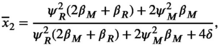
= 0.1. We begin by noting that the product margins do not tell the entire story; indeed, higher product margins are of no benefit if it causes demand to crater in the process. For this reason, we instead consider the real margins that take demand into account, which we defined earlier as

Real Margins vs. Transport Costs Under Linear Demand [Color figure can be viewed at
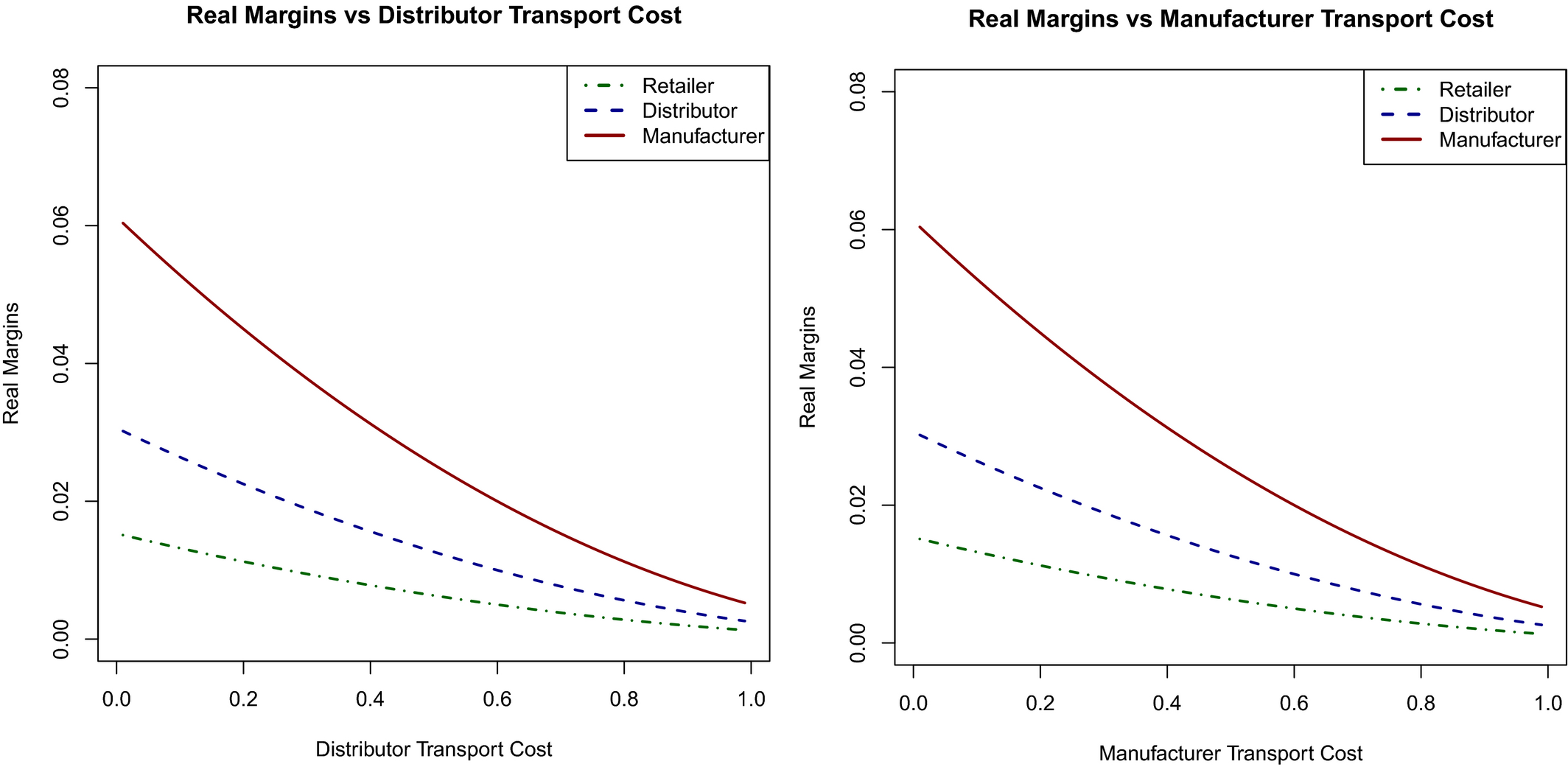
Real Margins vs. Transport Costs Under Isoelastic Demand [Color figure can be viewed at
We find that once the demand is taken into account, the players do not benefit from increased transport costs; indeed, transport costs eat into the players’ real margins under both linear and isoelastic demands. Note that, in contrast, this is not necessarily true for all of the players’ product margins. For instance, we can see from Proposition 2 that the manufacturer's product margin (


Model Comparison
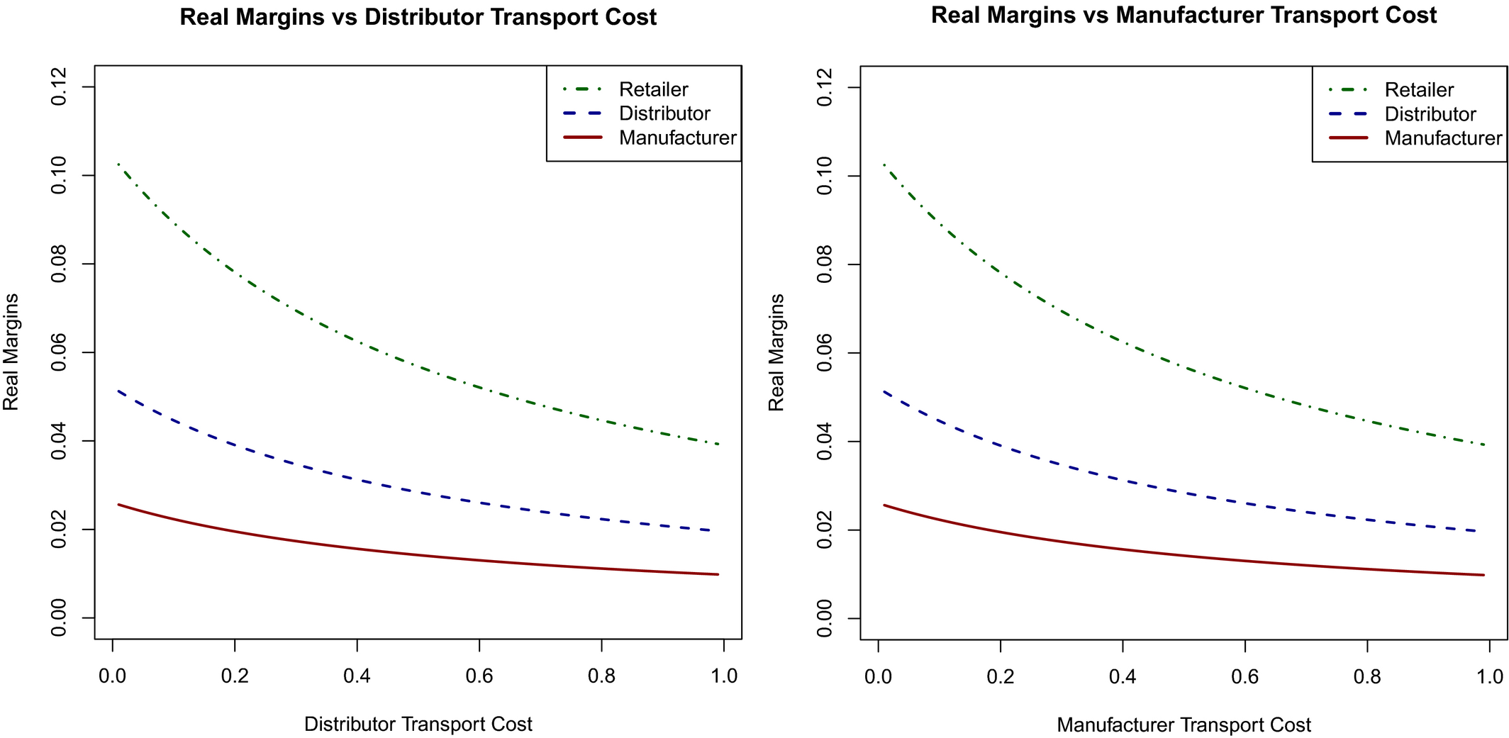
We now compare the two‐ and three‐echelon models assuming that the presence of the distributor reduces the transportation cost to some degree. More specifically, we assume that the parameter ξ in Equation (9) which represents all transportation cost savings due to the addition of the distributor is strictly positive. We then consider three different ratios to measure the benefit of the distributor. In particular, we consider the relative retail price (RRP), the relative retail margin (RRM), and the relative manufacturer margin (RMM), which we define as


By construction, the RRP measures the benefit to consumers, who wish to pay as little as possible for the product in question. For this reason, when the retail price under the three‐echelon model yields a lower price than that under the two‐echelon model, RRP would be greater than 1. On the other hand, the RRM and RMM measure the benefit to the retailer and the manufacturer, respectively. When their values are less than 1, then the three‐echelon model yields higher real margins for the retailer and the manufacturer relative to the two‐echelon model. For illustration, we plot each of these ratios against ξ, for 0 < ξ < 1, under both the linear and isoelastic demand functions in Figures 3–5.
Relative Retail Price Plots for Linear (red) and Isoelastic (green) Demand Functions [Color figure can be viewed at
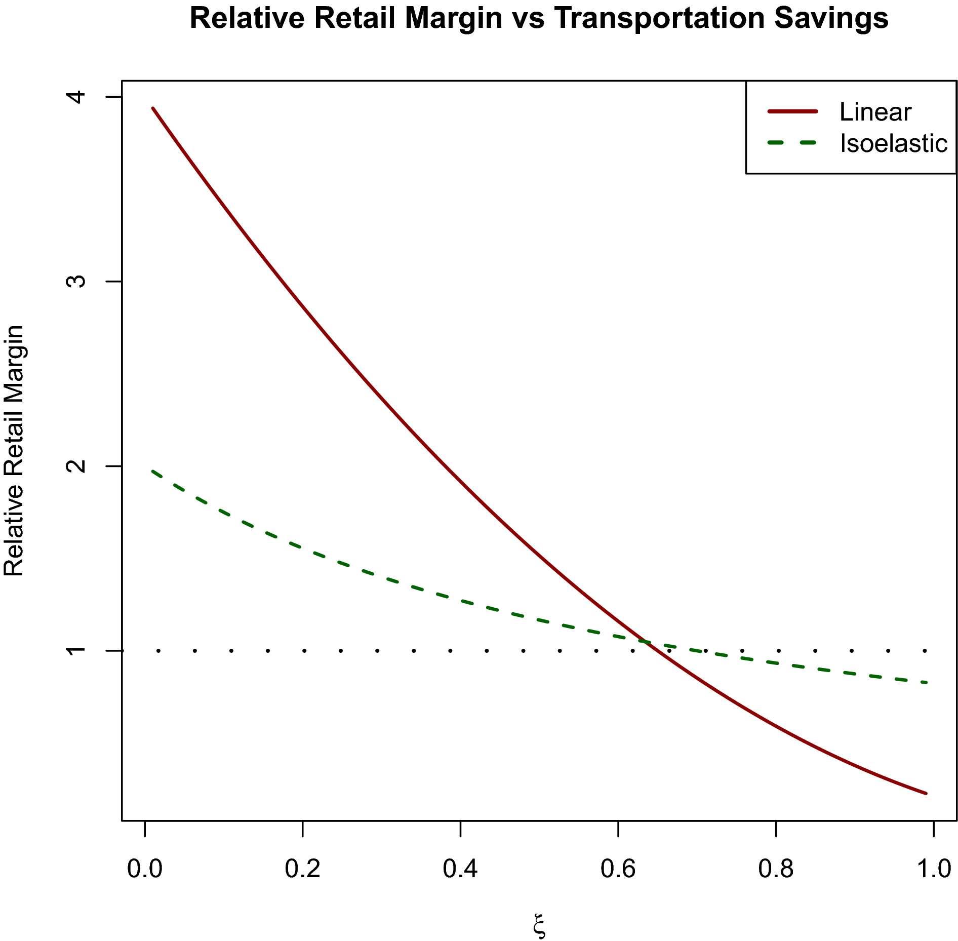
Relative Retail Margin Plots for Linear (red) and Isoelastic (green) Demand Functions [Color figure can be viewed at
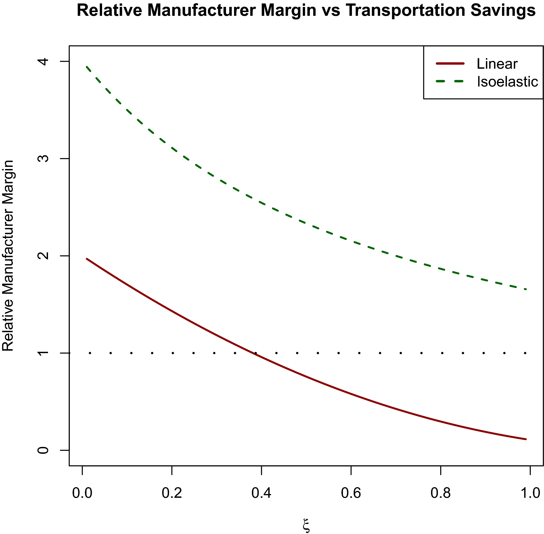
Relative Manufacturer Margin Plots for Linear (red) and Isoelastic (green) Demand Functions [Color figure can be viewed at
First, in Figure 3 we see that the RRP is increasing with ξ under both linear and isoelastic demand functions. Thus, provided the transport cost savings are sufficiently large, the consumer will benefit from the addition of the distributor through a reduced retail price. Interestingly, we find that the RRP is significantly more sensitive to the value of ξ in the case of isoelastic demand compared to linear demand. Second, in Figure 4 we see that RRM is decreasing with ξ in both the linear and isoelastic demand cases. Thus, provided the transport cost savings are sufficiently large, the retailer benefits from the addition of the distributor via an increased real margin. Importantly, however, we find that the RRM is more sensitive to ξ under the linear demand case, in stark contrast to the RRP. Finally, in Figure 5 we see that RMM is decreasing with ξ in both the linear and isoelastic demand cases. Thus, provided the transport savings are sufficiently large, the manufacturer benefits from the addition of the distributor via an increased real margin. However, in contrast to the RRM, we find that ξ needs to be significantly larger under isoelastic demand in order to yield RMM < 1. This reinforces our finding that the benefit of the distributor depends critically on the nature of the demand function.
Thus, both players always benefit from transport cost savings through increased real margins, provided the savings are sufficiently large. What is less clear is the exact amount of savings required, represented by ξ, for the distributor's presence to be beneficial to each player. In this respect, the following results identify explicitly the critical values of the parameter ξ beyond which it would yield positive savings to each player when the distributor is introduced to the supply chain.
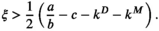
If the demand function is linear of the form Equation (5), then RRP > 1 if and only if

If the demand function is linear of the form Equation (5), then RRM < 1 if and only if

If the demand function is linear of the form Equation (5), then RMM < 1 if and only if
Propositions 19–21 highlight an important difference between the linear and isoelastic demand cases. Under linear demand, the distributor's presence will benefit the retailer, the manufacturer, and consumers if the transport cost savings ξ are sufficiently large relative to the difference between the theoretical maximum price, a/b, and the total cost of producing and shipping the product. In contrast, under isoelastic demand, consumers will benefit provided ξ is sufficiently large relative to the total cost of producing and shipping the product.
Advertising
Effect of Margins on Optimal Strategies
Similar to the values used in He et al. (2009), we take ρ = 0.1 and δ = 0.4, and also take ψ R = 0.5, ψ D = 0.25 and ψ M = 0.25, so that local advertising is the most effective channel. Unless otherwise stated, we take the player margins to be the optimal margins under linear demand when a = 1, b = 2, k D = 0.1, k M = 0.1 and c = 0.5, which yields m R = 0.0132, m D = 0.0264, and m M = 0.0528. All results are also replicated under isoelastic demand with ν = 5, which yield identical conclusions, and so we relegate the isoelastic case to Online Appendix B for brevity. In each plot, we let one player's margin vary, while fixing the remaining two at the values stated above, to ascertain the effect of each player's margin on the equilibrium advertising strategies. Note that the sufficient condition (33) is satisfied for all values considered in this section, so that provision of subsidy is optimal and Equations (27)–(29) are solved.
We begin by studying how each players’ margin affects the manufacturer's long‐run optimal participation rate ϕ*(t). The plots given in Figure 6 show that as the retailer's margin increases, the retailer has a higher incentive to advertise, and thus does so. This in turn reduces the incentive of the manufacturer to subsidize, due to the diminishing marginal returns of advertising. As a result, we see that the manufacturer's optimal participation rate decreases as the retailer's margin increases. Additionally, we find that the optimal participation rate is largely independent of the distributor's margin, although upon closer inspection we observe that it decreases negligibly with the distributor's margin. This can also be explained by noting that increasing the distributor's margin encourages the distributor to advertise more, which in turn reduces the manufacturer's marginal return of subsidizing the retailer. Finally, as expected we see that the optimal participation rate is increasing as a function of the manufacturer's margin, since the manufacturer has a higher incentive to grow market awareness.
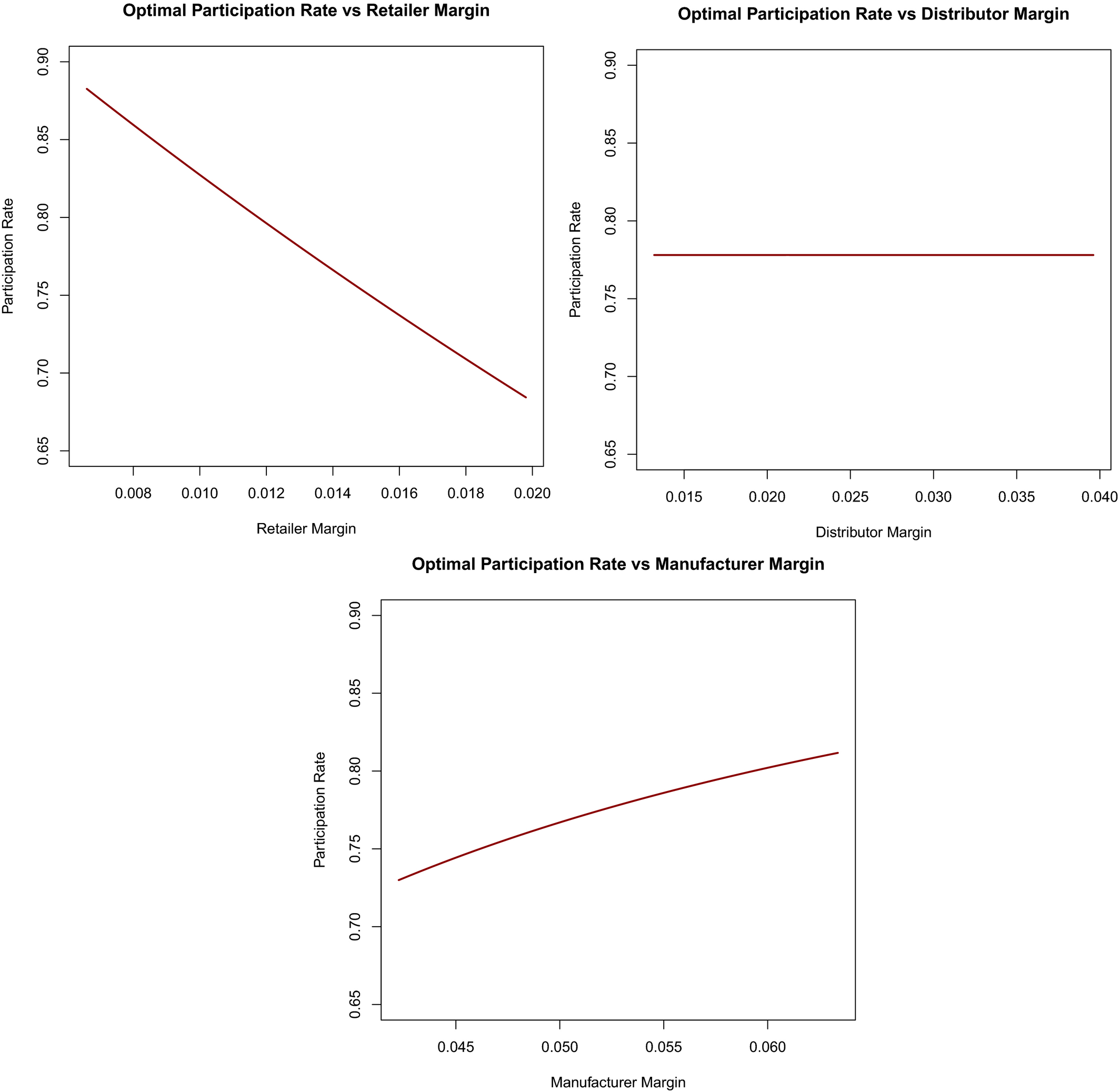
Effect of Player Margins on the Optimal Participation Rate [Color figure can be viewed at
Figure 7 shows the relationship between each of the advertising effectiveness parameters and the manufacturer's optimal participation rate under the three‐echelon model. Note that the scale has been enlarged to show the shape of each plot; in reality, the participation rate barely changes over the range of values considered. The results echo those of Figure 6; by increasing the retailer's advertising effectiveness, the retailer is encouraged to advertise more, and thus the manufacturer subsidizes less due to the decline in marginal returns. The optimal participation rate is also largely independent of the distributor's advertising effectiveness, although upon closer inspection we observe that it declines negligibly as the effectiveness increases since more effective advertising by the distributor increases the market awareness, causing a decline in the marginal return of the manufacturer's subsidy. Most interesting, however, is that the participation rate increases with the manufacturer's advertising effectiveness. Intuitively we would expect that as ψ M increases, the manufacturer would subsidize less as it diverts resources to the more effective national advertising channel. Instead, the manufacturer responds by subsidizing the retailer even more. To understand why this is, we refer to Figure 8, which shows the effect of changing the manufacturer's advertising effectiveness on each player's optimal advertising effort. As expected, increasing ψ M results in α M (t) increasing correspondingly; however, we also see a negligible decrease in both α R (t) and α D (t) due to the manufacturer's increasing effort reducing the marginal return of advertising. Thus, as the retailer's advertising effort decreases, the manufacturer increases its participation rate to compensate since, all else being equal, the marginal return of advertising through the local advertising channel is now higher.
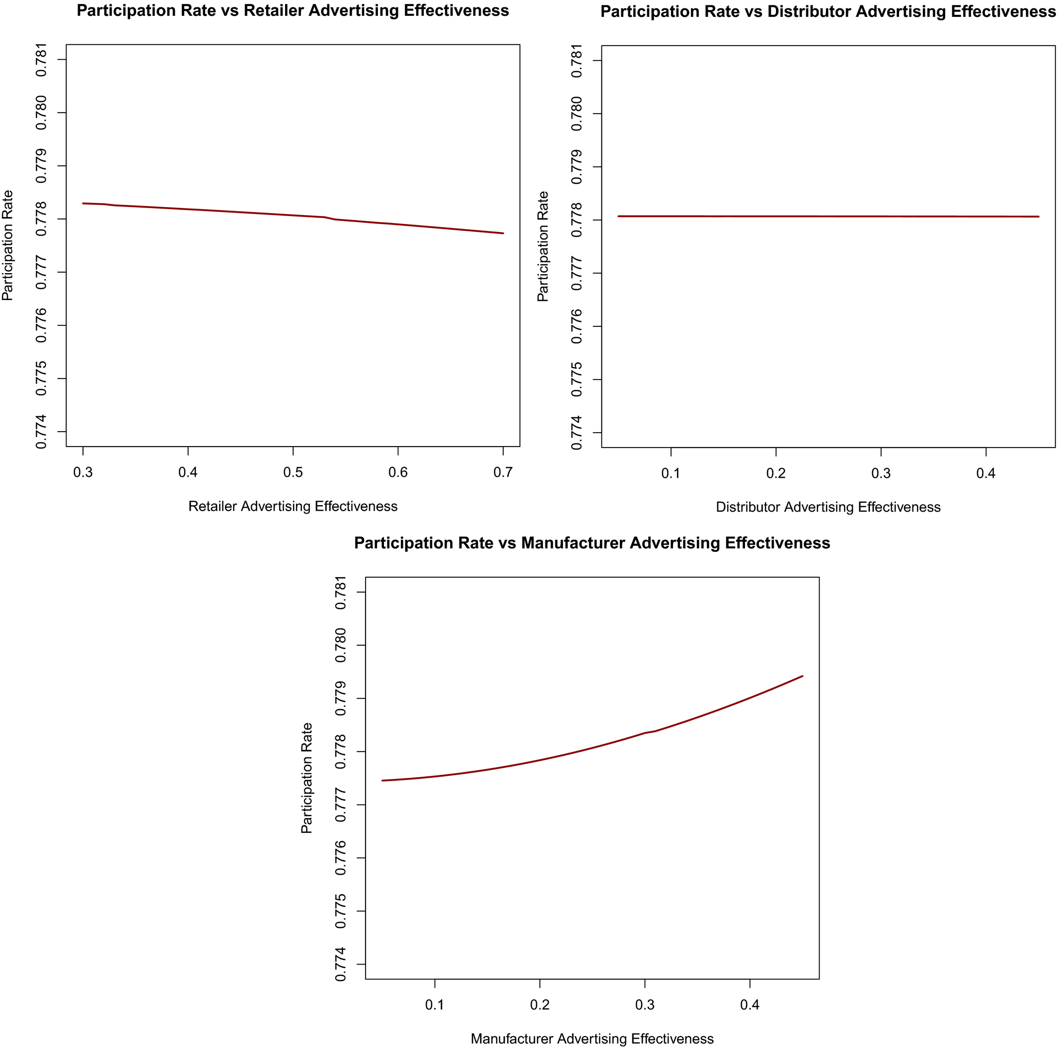
Effect of Advertising Effectiveness on the Manufacturer's Participation Rate [Color figure can be viewed at
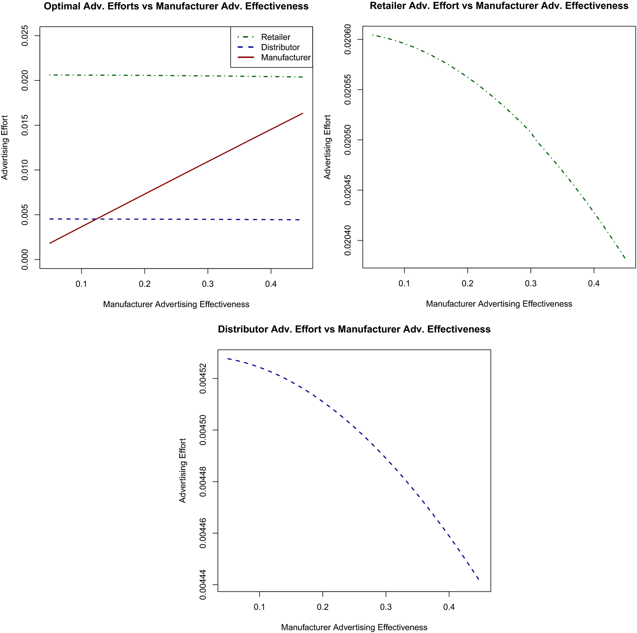
Effect of the Manufacturer's Advertising Effectiveness on the Optimal Advertising Efforts [Color figure can be viewed at
Next, we examine how the player margins affect the optimal advertising efforts


The Relationship between Player Margins and their Optimal Advertising Efforts
These results highlight the role that co‐op advertising plays in aligning the incentives of supply chain members and more equitably distributing the burden of advertising. We see that without any co‐op advertising program, increasing one player's margin will generally result in no change to the remaining players’ advertising strategies. However, by introducing a co‐op advertising program, increasing the margin of the manufacturer will also increase the retailer's advertising effort due to the manufacturer increasing its participation rate. This benefits the supply chain as a whole since the manufacturer is able to tap the local advertising channel via the retailer, rather than relying solely on national advertising, reducing the impact of advertising saturation.
Model Comparison
In this section, we compare the two‐ and three‐echelon models to investigate whether the addition of the distributor has any tangible benefit to the supply chain as a whole. Once again, we consider a parameter ξ to represent transport cost savings defined in the previous pricing section. The derived coupled equations depend on ξ through the optimal player margins


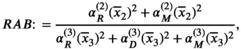
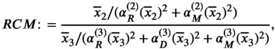
To compare the models, we consider several different metrics based on the long‐run mean of each model given in Equations (35) and (45) since the long‐run mean best characterizes the general behavior of the players. The metrics considered are the relative advertising budget (RAB)

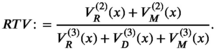
The RTV is evaluated using initial market awareness levels x = 0.1, 0.5, 0.9 to examine whether the relative performance of the models is sensitive to the initial conditions. We calculate each of these metrics as we vary the transport cost savings parameter ξ, thus demonstrating how transport cost savings offered by the distributor benefits the supply chain as a whole. Figure 10 shows the RAB under both linear and isoelastic demands plotted against ξ. Unsurprisingly, RAB is seen to be monotonically decreasing in ξ under both linear and isoelastic demands. As the transport cost savings obtained by the distributor's presence increases, the three‐echelon model reinvests these savings into advertising, thus increasing its advertising expenditure relative to the two‐echelon model. This difference then appears to level off exponentially as ξ increases further. Indeed, this leveling off is expected due to the diminishing returns of advertising under the Sethi model.
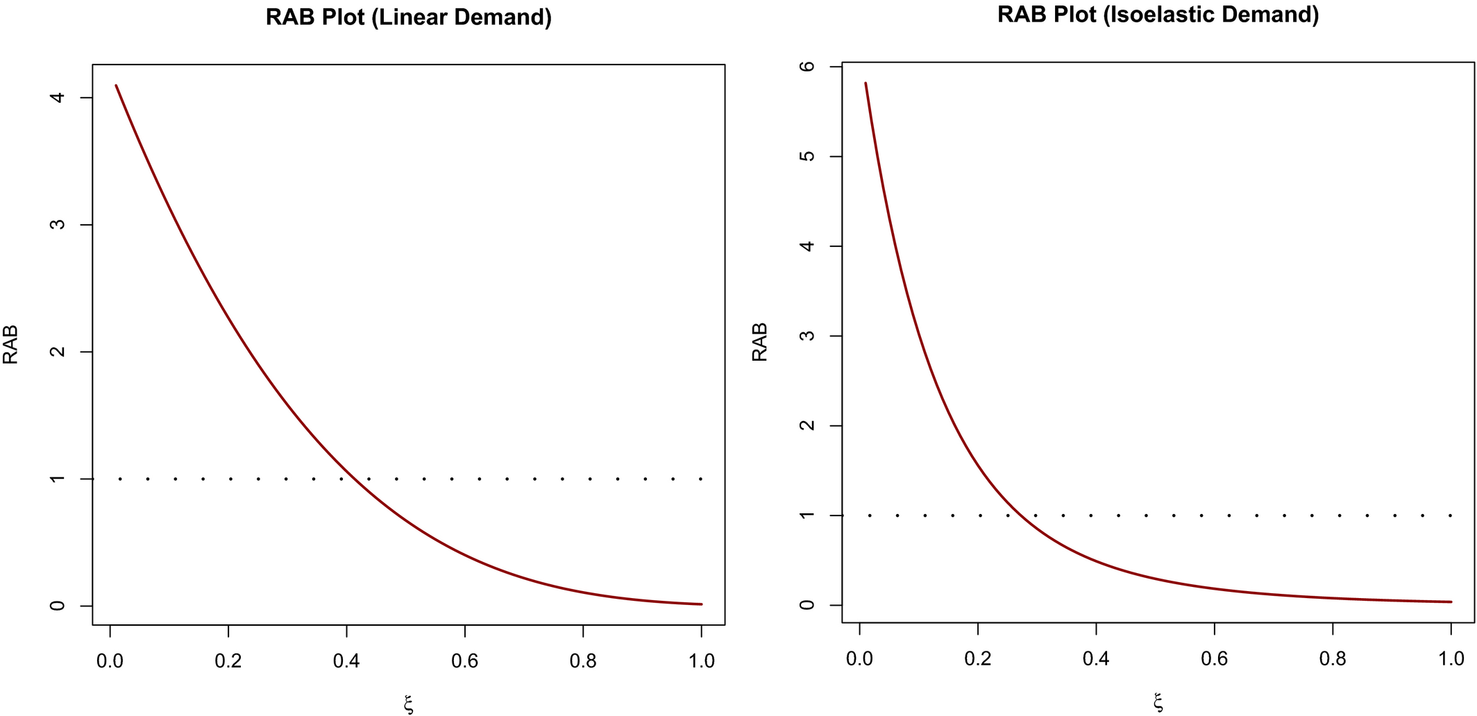
Relative Advertising Budget vs. ξ under the Linear (left) and Isoelastic (right) Demand Functions [Color figure can be viewed at
In Figure 11 we similarly find that RMA is monotonically decreasing in ξ. As we increase ξ, the three‐echelon model can invest more in its advertising efforts, as shown in Figure 10, and thus the long‐run market awareness also increases relative to the two‐echelon model. This finding is also consistent with the plots of RCM given in Figure 12, in which we find that RCM is monotonically increasing with ξ. This suggests that as ξ increases, the three‐echelon model is paying more to maintain its long‐run market awareness compared to the two‐echelon model, which is due to the diminishing returns that it encounters as it invests more in advertising relative to the two‐echelon model.
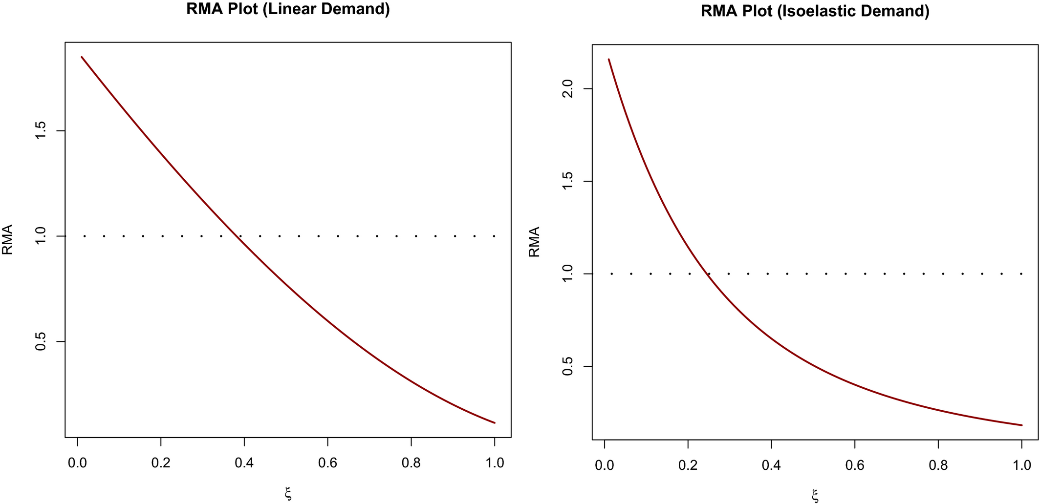
Relative Market Awareness vs. ξ under the Linear (left) and Isoelastic (right) Demand Functions [Color figure can be viewed at
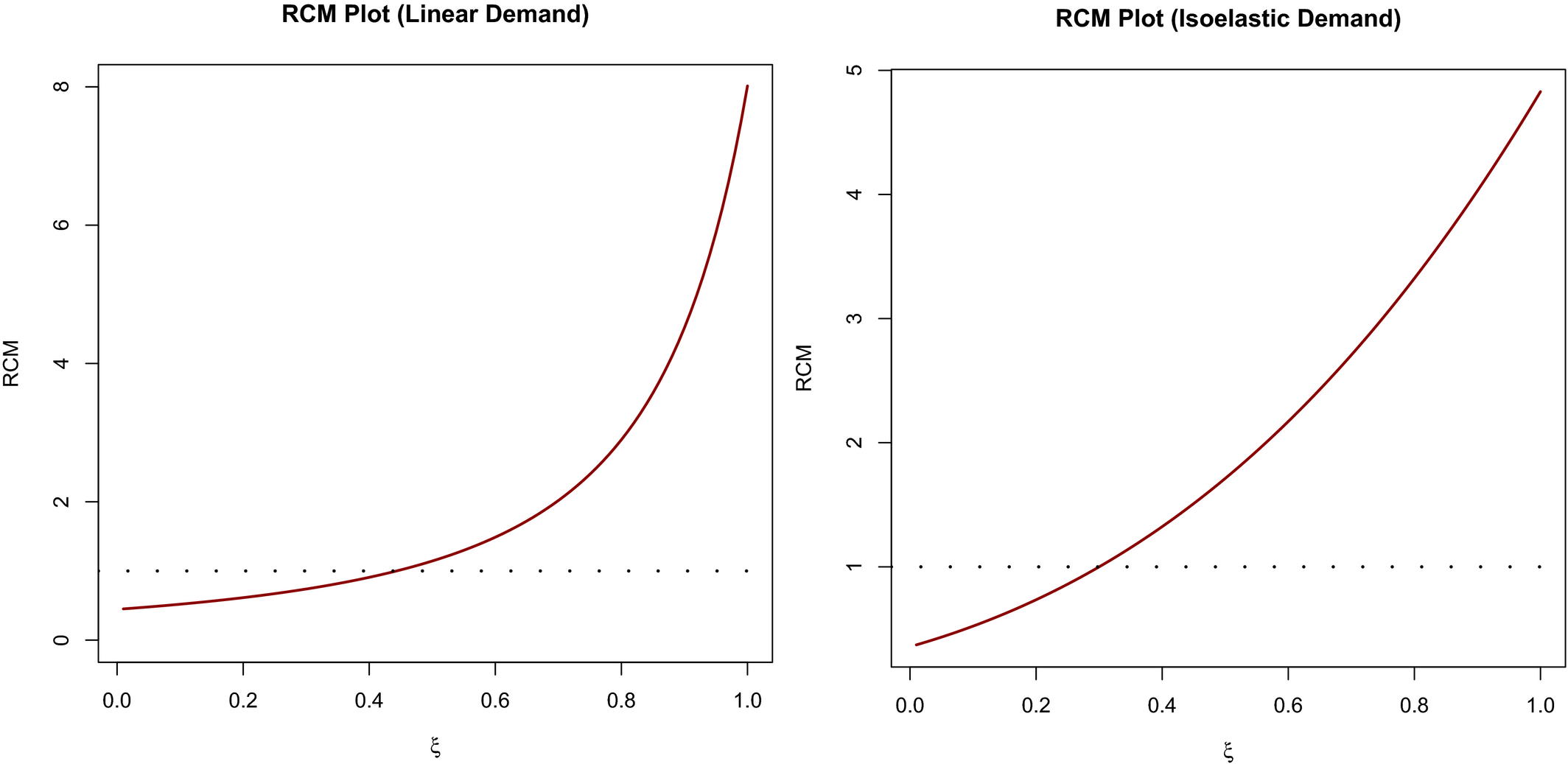
Relative Cost Per Market Awareness vs. ξ under the Linear (left) and Isoelastic (right) Demand Functions [Color figure can be viewed at
In Figure 13, we see that RTV is also decreasing with ξ, suggesting that the transport cost savings enable the supply chain to extract more value overall. Importantly, the three‐echelon model extracts more value than the two‐echelon model once ξ ≈ 0.3 and ξ ≈ 0.2 under both linear and isoelastic demands, which is not prohibitively large relative to k D , k M , and c. Moreover, this result holds for all three values of x considered, demonstrating that these results are robust to the initial market awareness. Indeed, this demonstrates that despite the additional marginalization the distributor's presence causes, the three‐echelon supply chain might still realistically be able to extract more value provided the transport cost savings are sufficiently large. An important question is whether these results still hold when the RTV is evaluated at each model's respective steady‐state equilibrium, rather than the initial market awareness since these are the market awareness levels each model will occupy over the long term. As it turns out, evaluating the RTV at each model's steady‐state yields identical conclusions; the corresponding plots of the RTV evaluated at the steady‐state equilibria can be found in Online Appendix C.
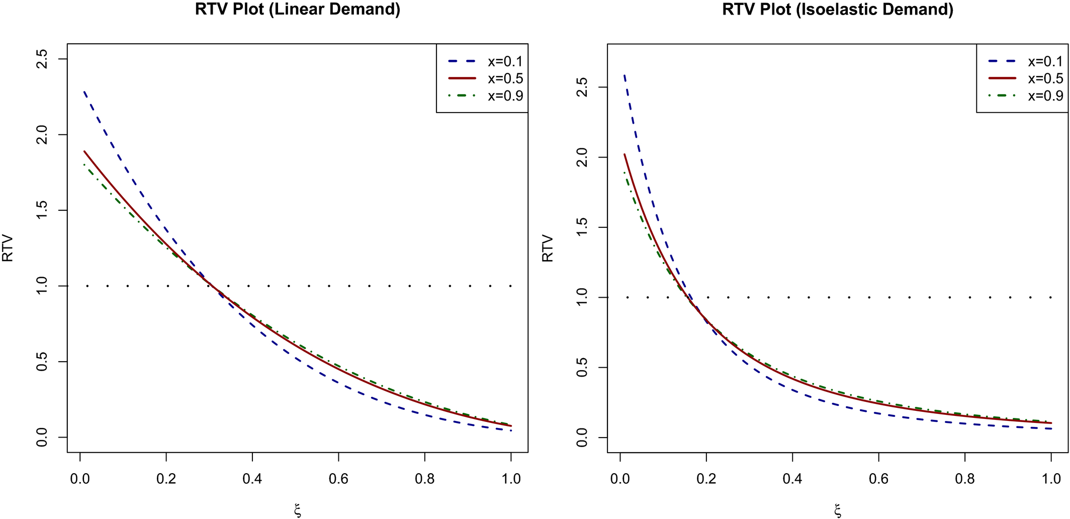
Relative Total Value vs. ξ under the Linear (left) and Isoelastic (right) Demand Functions [Color figure can be viewed at
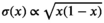
Finally, in Figure 14, we generate sample paths of X
t
for both the two‐ and three‐echelon models (with subsidy) when x = 0.5 under linear and isoelastic demands, taking ξ = 0.6 for the two‐echelon case. To facilitate comparison, these sample paths are generated using the same Wiener process. The long‐run mean is superimposed in black to highlight the volatility brought about by the stochastic component σ(x), which we take as


Sample Paths of X
t
with Long‐Run Means (black) Superimposed under Linear Demand (left) with


Conclusion
In this study we have proposed a model to illustrate the value added by a distributor to a supply chain in its co‐op advertising and pricing programs. The motivation for having a distributor is to improve the transportation efficiency of the supply chain; that is, to reduce the costs associated with transporting product from the manufacturer to the retailer. We study this problem by assuming that the addition of the distributor results in transport cost savings, and then examined how these savings influence the players’ strategies, prices, and margins. We model the co‐op advertising and pricing problem among the retailer, distributor, and manufacturer as a dynamic Stackelberg game problem. In particular, an extension of the Sethi advertising model is used to describe the product's market awareness owing to its analytical tractability and empirical validation.
By embracing the tractability of the Sethi advertising model we are able to tackle the pricing and advertising problems separately. We first derive closed‐form expressions of the players’ optimal prices under both linear and isoelastic demand functions. We characterize the feedback Stackelberg equilibrium advertising decisions and the players’ value functions in terms of a solution of a coupled system of algebraic equations, and establish the existence of a unique solution under a mild margin condition on the manufacturer and the retailer. In addition, we also establish sufficient and necessary conditions for the subsidy to be optimally provided to the retailer. It is important to mention that the inclusion of national advertising in the co‐op program under the Sethi model is relatively new to the literature, having only been explored numerically by Bensoussan et al. (2019) under the mixed leadership framework, whereas we provide a detailed analysis. In summary, the theoretical results in this study represent a significant theoretical contribution to dynamic Stackelberg advertising and pricing games with a distributor.
Our model demonstrates how the transport costs associated with both the distributor and manufacturer affect the optimal pricing and advertising strategies. Interestingly, we find that how the transport costs are absorbed by the supply chain depends fundamentally on the nature of the demand function, illustrated by the differing results for linear and isoelastic demands. In particular, we find that the manufacturer's transport cost is borne primarily by the manufacturer in the case of linear demand, while under isoelastic demand the manufacturer is able to pass it on to the other players. This is a significant finding as it suggests that companies must tailor how they absorb transport costs based on the demand curve of the product. We further verify that, under both linear and isoelastic demands, increased transport costs result in a higher retail price and lower real margins, thereby harming both the supply chain and the consumers.
Our numerical results show that each player's advertising effort increases with respect to its own margin. Furthermore, the retailer's advertising efforts increase with the manufacturer's margin, which can be explained by the increase in the manufacturer's subsidy to the retailer as the manufacturer's margin increases. Interestingly, we see that the manufacturer's subsidy to the retailer decreases slightly as the distributor's margin increases, since the distributor will advertise more as its own margin increases, which in turn implies that the manufacturer should not increase its subsidy to avoid the diminishing marginal return of advertising.
Using several key ratios we are able to compare our three‐echelon model with a corresponding two‐echelon model, that excludes the distributor, to study the value of the distributor and how this value manifests in the players’ optimal strategies. Under linear and isoelastic demands, we find that the addition of the distributor results in both a lower retail price and higher margins, provided the transport cost savings are sufficiently large. Importantly, we give explicit expressions for the transport cost savings necessary for the distributor to benefit each player. Thus, in addition to the results concerning the absorption of transport costs, we see that it is important for the supply chain to estimate the form of the demand function of the product using past sales data in relation to price changes, along with the knowledge that exists in the industry regarding the nature of the product demand.
Finally, there are several potential areas of further research that build upon our model. First, instead of considering co‐op advertising, one can also study the impact of co‐op selling by considering a salesforce hierarchical structure, which can be perceived as a dynamic extension of the hierarchical structure in Caldieraro and Coughlan (2007). Second, in this study we have considered only a supply chain consisting of a single product sold by a single retailer. A natural extension would therefore be to consider multiple competing retailers. The retailers would have different associated transport costs owing to their geographic proximity and order sizes, and therefore the strategies and the values they place on the distributor may differ substantially. Such a model would shed light on how adding a distributor can contribute to a supply chain with competing retailers. This would offer further insight into the role and value of distributors in an increasingly globalized world, where the transport costs to various markets can differ significantly. This idea could be taken further by considering the problem within a mean‐field Stackelberg game framework, as systematically studied in Bensoussan et al. (2013, 2015a, 2020). Along this same vein, we might also consider a manufacturer that produces competing products, say for example smartphones, that the competing brands have contracted with the manufacturer to produce. Such a model could offer insight to companies wishing to outsource manufacturing to low‐cost labor markets.
Footnotes
Acknowledgments
We thank the DE (Fred Feinberg), SE, and the two anonymous referees for their insightful comments. We also note that the SE suggested an enrichment of our model to study the problem of co‐op selling and consideration of competing echelons. We also thank Prasad Naik and Rong Zhang for their comments and suggestions on an earlier draft of this study. Adrian P. Kennedy acknowledges the Hong Kong University Grants Committee for their support of him pursuing his PhD at the Chinese University of Hong Kong, and that this work will constitute part of his dissertation. Suresh P. Sethi acknowledges the financial support from the Eugene McDermott Chair Professorship and he dedicates this work to the memory of his sister who left this world during the final revision stage of this study. Chi Chung Siu acknowledges that the work is supported by the grant “Generalized Sethi Advertising Model and Extensions” (Project No. UGC/FDS14/P02/20) from the Research Grants Council of the Hong Kong Special Administrative Region, China. Phillip Yam acknowledges the financial supports from HKGRF‐14300717 with the project title “New kinds of Forward‐backward Stochastic Systems with Applications,” HKGRF‐14300319 with the project title “Shape‐constrained Inference: Testing for Monotonicity,” HKGRF‐14301321 with the project title “General Theory for Infinite Dimensional Stochastic Control: Mean Field and Some Classical Problems,” Germany/Hong Kong Joint Research Scheme Project No. G‐HKU701/20 with the project title “Asymmetry in Dynamically correlated threshold Stochastic volatility model,” and Direct Grant for Research 2014/15 (Project No. 4053141) offered by CUHK. He also thanks Columbia University for the kind invitation to be a visiting faculty member in the Department of Statistics during his sabbatical leave. He also recalls the unforgettable moments and the happiness shared with his beloved father during the drafting of the present article at their home. Although he just lost his father at the final stage of the review of this work, his father will never leave the heart of Phillip Yam and he dedicates this work to the memory of his father's brave battle against liver cancer.