Besides using earmark budget to support farmer cost subsidies, governments in many developing countries use minimum support price (MSP) as an alternative subsidy scheme to (i) safeguard farmers' incomes against vagaries in crop price and (ii) ensure sufficient crop production. Among different MSP schemes, we focus on the credit‐based MSP scheme under which a government will not take any possession of a crop; instead, it will credit farmers if the prevailing market price is below the prespecified MSP. In this paper, we consider a market consisting of infinitesimally small, rational, and strategic farmers (with heterogeneous production costs) who face market and yield uncertainties. Our equilibrium analysis reveals that (i) although both cost subsidy and MSP induce more production, cost subsidy leads to a higher crop production than MSP; (ii) MSP improves farmer's and consumer's surpluses; however, cost subsidy improves consumer's surplus but it can decrease farmer's surplus, which is unexpected; (iii) although both programs achieve the same optimal net value (i.e., sum of farmer's and consumer's surpluses minus shortage cost and expenditure), MSP always offers higher farmer's surplus than cost subsidy; and (iv) it is beneficial to invest only in cost subsidy, in both cost subsidy and MSP, and only in MSP, when the budget availability is low, moderate, and high, respectively, so that the net surplus (i.e., sum of farmer's and consumer's surpluses less the shortage cost) is also maximized along with the net value generated being maximized.
Agriculture is the main source of income for many in developing countries. In India, 70% of rural households depend primarily on agriculture for their livelihood, with 82% of farmers being small and marginal (FAO, 2020). According to the Ministry of Agriculture and Farmers Welfare, Government of India (2019), the average farm size in India is about 1 ha (=2.47 acres) and marginal and small landholders constitute 86.21% of the total landholders in India (Krishnan, 2018). A similar situation exists in developing countries such as Africa, Indonesia, Pakistan, Turkey, Thailand, and others. Smallholders (or small farmers) constitute a major portion of the farmers in many developing countries. Despite the small‐sized landholdings of these farmers, 500 million smallholder farmers in the world produce up to 80% of the food consumed in Africa and Asia (African Smallholder Farmers Group (ASFG), 2013).
To sustain small farmers' operations, governments of developing countries offer various programs to support and protect their income. A common farmer‐support program is input cost subsidies, wherein a government offers financial assistance to farmers by bearing a fraction of the farmers' cultivation costs. Input subsidy programs (ISPs) are adopted by many emerging economies such as Africa and India. In Africa, smallholder farmers are issued coupons that they can redeem for input packets from both government and private vendors (Jayne et al., 2018). In India, central and individual state government subsidies for seeds, irrigation, power, and fertilizers are offered to farmers (see Hemming et al., 2018, and the references therein).
Besides cost subsidy, an alternative support program is the credit‐based minimum support price (MSP; also known as deficiency payment). Under a credit‐based MSP, a government will not take any possession of the crop; instead, it will provide a monetary credit to farmers cultivating the crop if the prevailing market price of the crop is below the prespecified MSP. For example, in India, credit‐based MSPs are currently offered for eight crops (mostly oilseeds and legumes) for which the Indian government takes no (or very low) possession of crop (Bera, 2017).
Motivated by the credit‐based MSP program launched in India recently, we are interested in developing a model to compare the effectiveness of (i) cost subsidies and (ii) credit‐based MSP in the presence of (risk‐neutral) advisory bodies that guide farmers to make crop choice decision in a risk‐neutral manner.1 Our intent is to examine the following research question: Given cost subsidy is common, will MSP outperform cost subsidy in terms of value creation in the presence of market and crop‐yield uncertainties?
To facilitate our analysis, we develop a Stackelberg game‐theoretic model to capture the underlying dynamics between government (that sets the cost subsidy or MSP for a focused crop) and price‐taking small farmers (who decide on their production quantities in a risk‐neutral manner).2 In our model, we assume that farmers have heterogeneous crop production costs, which is a crucial factor that influences farmers' sowing decisions. The farmers are rational and strategic so that they make their crop‐sowing decisions based on the anticipated future (equilibrium) price of the crop after considering all the other farmers' decisions. To capture demand and supply uncertainties, we assume (i) exogenous market uncertainty and (ii) crop production yield uncertainty.
By comparing the equilibrium outcomes associated with cost subsidy and MSP, we find:
Both cost subsidy and MSP induce more production; however, cost subsidy entices more farmers to sow a crop than MSP. The total production quantity of a crop always increases in the cost subsidy or MSP. Additionally, for any earmarked budget, the crop production is higher under cost subsidy than that under MSP.
MSP improves farmer's and consumer's surpluses; however, cost subsidy improves consumer's surplus, but it can negatively impact farmer's surplus. Despite this difference, both cost subsidy and MSP increase the total surplus, which we define as the sum of farmer's and consumer's surpluses.
Both cost subsidy and MSP achieve the same maximum net value (which we define as the sum of farmer's and consumer's surpluses minus the shortage cost and the expenditure incurred); moreover, MSP offers higher farmer's surplus but at a higher expenditure. However, it is better to opt for cost subsidy than MSP when the budget available is low.
Hybrid policy (combined cost‐subsidy and MSP policies). Hybrid policy generates the same optimal net value as standalone cost‐subsidy policy or MSP policy. It is beneficial to invest only in cost subsidy if the budget availability is low, in both cost subsidy and MSP if the budget availability is moderate, and only in MSP when the budget availability is high, so that the net surplus (i.e., sum of farmer's and consumer's surpluses less the shortage cost) is also maximized along with the net value generated being maximized.
While the first result is as expected, the second result on cost subsidy is unexpected. The second finding shows that cost subsidies could degrade farmer's surplus even though government defrays a fraction of each farmer's cultivation cost. However, the third finding informs that both cost subsidy and MSP can achieve the same maximum net value in the absence of budget constraint, although it is true that MSP always achieves higher farmer's surplus than cost subsidy, but at a higher expenditure. Finally, our last finding indicates that the maximum net values that can be achieved through (i) standalone cost subsidy, (ii) hybrid policy, and (iii) standalone MSP are all equal, although each option offers different farmer's surpluses at different expenditures (with (iii) offering the highest farmer's surplus at the highest expenditure).
Our paper is organized as follows: We review relevant literature in Section 2 and provide model preliminaries in Section 3. In Section 4, we examine the base case to form a benchmark and in Sections 5 and 6 we analyze the impacts of cost subsidy and MSP in the presence of price uncertainty, respectively. We also determine the optimal MSP and cost subsidy that maximize the net value generated. Then, in Section 7, we compare the performance of cost subsidy against MSP and discuss how a policymaker should choose between the two policies for any specific budget availability. Lastly, in Section 8, we examine how a stipulated budget should be apportioned between cost‐subsidy and MSP schemes in order to maximize net surplus along with net value derived from a hybrid policy. In Section 9, we conclude the paper and provide a few prospective directions for future research. We provide a few supplementary results in Appendixes A–C and provide the proofs of all our results in the Supporting Information of this paper.
LITERATURE REVIEW
We first review some papers related to farmer cost subsidies that belong to ISPs (Jayne et al., 2018). Cost subsidies can occur in different forms; for instance, the governments in Mali, Ghana, Nigeria, and other such African countries offer subsidies for seeds and fertilizers to smallholder farmers (Brooks & Wiggins, 2010; Jayne & Rashid, 2013; Jayne et al., 2018). In India, subsidies are offered not only on direct inputs such as seeds and fertilizers (Prasad, 2016) but also on other resources such as power and irrigation by both central and state governments (Bardhan & Mookherjee, 2011; Fan et al., 2008). Xu et al. (2009) find that fertilizer subsidies may reduce or surge the commercial demand for fertilizers in the area depending on whether the private sector is active or inactive. Chibwana et al. (2012) show that input subsidies can entice farmers to allocate more land to those subsidized crops in Malawi. We refer the readers to Hemming et al. (2018) for a comprehensive review of the various types of input subsidies provided to smallholder farmers.
Next, the agricultural economics literature on MSPs is vast; see Tripathi et al. (2013) for a comprehensive review. Fox (1956) develops an economic model to evaluate the impact of MSPs and finds that MSPs can mitigate the fall in gross national product during a recession. Dantwala (1967) finds that, in spite of the increasing MSPs, crop's market prices continue to rise because procurement‐based MSPs form a lower bound to market prices (Ramaswami et al., 2018; Subbarao et al., 2011). Chand (2003) presents a qualitative assessment of the ill effects of wheat‐and‐rice‐centric procurement‐based MSPs on the Indian economy. Besides those examining MSP in the Indian context, Spitze (1978) analyzes the impact of federal policy (The Food and Agriculture Act of 1977) on agriculture in the United States. Dean (1996) describes the Brannan plan (a credit‐based MSP) and Innes (1990) examines the impact of Brannan plan on a nonstrategic monopolist farmer. This observation motivated us to examine the efficacy of the credit‐based MSP scheme for achieving its intended goals (i.e., farmer welfare and crop availability) when farmers are small and strategic and compare the performance of MSP against the more common input subsidy scheme.
There has been a recent interest in operations management that examines social responsibility and public policy issues arising in agriculture. Hu et al. (2017) show that a tiny fraction of strategic farmers can stabilize the steady‐state crop prices without considering MSP. Alizamir et al. (2018) focus on the impact of two schemes (price loss coverage and agriculture risk coverage programs different from MSP) on (i) farmers' welfare, (ii) federal expenditure, and (iii) consumer's welfare. Recently, Guda et al. (2021) and Ramaswami et al. (2018) examine the role of procurement‐based MSPs in emerging economies by considering homogeneous production costs while Chintapalli and Tang (2020) examine the impact of credit‐based MSPs in the presence of market and yield uncertainties and when farmers are risk‐averse and possess heterogeneous production costs. More recently, Akkaya et al. (2021) examine the role of governmental support policies in farmers' adoption of innovative production methods in agriculture.
Unlike Guda et al. (2021) and Ramaswami et al. (2018) who focus on procurement‐based MSP scheme, we focus on credit‐based MSP scheme in the presence of crop's market‐price uncertainty when the crop cultivation costs are heterogeneous among farmers.3 Next, although our paper is close to Chintapalli and Tang (2020), we focus on and study different issues in this paper as follows.
First, Chintapalli and Tang (2020) analyze only the MSP scheme as a standalone program, while we study both MSP and cost subsidy as well as the hybrid policy that combines both cost subsidy and MSP. Also, we compare the performance of MSP against cost‐subsidy scheme. Second, Chintapalli and Tang (2020) examine the role and impact of MSP when farmers are “highly” risk‐averse. However, they do not address the case when farmers are risk‐neutral, which is important especially with the increasing presence of farmer cooperatives, NGOs, and other governmental and educational advisory bodies that provide informational support and guidance to farmers in the choice of crop to show in a risk‐neutral manner thereby reducing their risk‐aversion. Therefore, the role of MSPs (that is also implemented by government) in confluence with such farmer‐advisory programs remains to be assessed, in order to obtain a holistic impact of MSPs when farmers take decisions in a risk‐neutral manner. Third, in our paper, apart from evaluating and comparing the impact of credit‐based MSP and input cost subsidies on all the stakeholders—farmers, consumers, and government (or policymaker)—we also analyze the scenario when both cost subsidy and MSP are offered simultaneously, through a hybrid policy.
MODEL PRELIMINARIES
To capture the characteristics of smallholder farmers in developing countries, we assume that farmers are infinitesimally small so that a farmer cannot influence the market price individually and each farmer is a price taker (Liao et al., 2017). For ease of exposition, we scale the total “input production capacity” in the market (i.e., the total input available across all farmers) to 1 unit and all farmers have equal input production capacity (i.e., the 1 unit input production capacity in the market is equally distributed among all farmers). Furthermore, we assume that each farmer is risk‐neutral and the farmers do not collude among themselves (Chintapalli & Tang, 2020).
Heterogeneous production cost
In our model, we account for heterogeneity in the unit cost of crop cultivation among farmers; that is, the cost incurred by each farmer to cultivate a “unit input capacity.” In this paper, we use the term “unit production cost” of a farmer to refer to the cost incurred by the farmer to cultivate a unit input capacity. We model the cost heterogeneity among farmers using the linear‐city model on the unit interval
(Chintapalli & Tang, 2020; Liao et al., 2019; Mendelson & Parlaktürk, 2008; Tirole & Jean, 1988). Hence, we make the following assumption:
All farmers are uniformly distributed over
with respect to their unit production cost
.
In view of our modeling Assumption 1, we scale the total population of infinitesimally small farmers to 1 unit and, therefore, the total production capacity that is available across all the farmers together is scaled to 1, because the capacity of each farmer is scaled to 1 (Xiao et al., 2020).
Each farmer has two options: (i) to sow the focused crop (along with the quantity to sow) or (ii) to not sow the focused crop. We scale the profit of the latter option to
(which corresponds to an outside option like the case when a farmer grows a “stable” crop with stable price and stable yield). The profit of a farmer is determined by ex post market price of the focused crop, while the cost of cultivation is incurred ex ante by the farmer.
Impact of agricultural policies
We examine the impact of cost subsidy and MSP on three competing measures: (1) farmer's surplus (
), (2) consumer's surplus (
), and (3) net value (
) of the corresponding program—cost subsidy or MSP. The “net value”
created by the associated program is defined as
, where
denotes the shortage cost that is incurred due to unsatisfied demand and
denotes the implementation cost of a program. We let
,
,
, and
denote farmer's surplus, consumer's surplus, shortage cost, and net value, respectively, in the absence of any support program.
Demand model
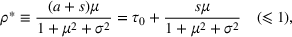
In this paper, we analyze the impact of cost subsidy and MSP when the crop price is uncertain due to two types of uncertainties: (i) market uncertainty and (ii) crop‐yield uncertainty. To capture these uncertainties and to obtain tractable results, we assume that the crop's market price satisfies
Here, the random variable
denotes the market uncertainty, which is an exogenous noise in the crop's price that is independent of the quantity of the crop available (Chintapalli & Tang, 2020; Huang et al., 2013; Mills, 1959; Petruzzi & Dada, 1999), and the random variable
denotes the crop's production yield uncertainty factor at the “market level” that is resultant of the aggregation of individual farmer yields. While
captures the impact of various macroeconomic factors and changes in consumers' tastes,
captures the variability in production yield due to environmental factors and agricultural practices such as rainfall and irrigation, infestation of pests and diseases, and quality of seeds and other farm inputs.
To ensure technical tractability and to focus our analysis on the impact of cost subsidy and MSP on stakeholders, we assume that all farmers have the same individual yield
, which is also the market‐level yield. Such an assumption of “perfectly correlated” yields among farmers is commonly adopted in the literature to ensure technical tractability. Such an assumption is reasonable when the circumstances of crop cultivation are similar among farmers, as explained in Alizamir et al. (2018) and Kazaz and Webster (2011). This assumption is also justifiable in practice, especially when farmers adopt high‐quality farm inputs and improved farming practices to generate a conducive environment for crop cultivation (NITI Aayog, 2016).4
Therefore, the “total output quantity” of crop available for sale in the market, when a total input capacity of
is involved in crop production, is
. In other words, the crop's market price is given by
, where
is the total quantity of the crop available for a realized yield of
.
We assume that the random variables
and
are independent and we denote their density functions by
and
, respectively. Furthermore, without loss of generality, we let
, Var
,
, and Var
. Therefore, the crop's average output quantity is
and its average market price is
when a total input capacity of
is invested. Finally, we make the commonly used nonrestrictive assumption that the market potential
is sufficiently high so that the crop's market price is nonnegative (Chintapalli & Tang, 2020; Petruzzi & Dada, 1999).
Lastly, throughout our analysis we adopt the following common notation that
and
, and we denote the per unit crop shortage cost by
.
BENCHMARK CASE (NO SUPPORT PROGRAM)
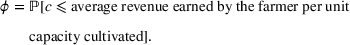
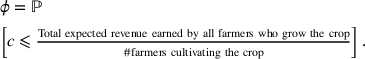
In this section, we examine the benchmark case when no support program is available. Under rational expectation, a risk‐neutral farmer with unit production cost
will cultivate the crop if and only if the expected unit revenue is higher than the cost of cultivating the crop.5 Because the farmers are uniformly distributed on
with respect to their cultivation costs, the fraction
of farmers who sows the focused crop in equilibrium under rational expectation of farmers is given by
Because we had scaled the farmer population to 1 and the total market capacity to 1 unit,
also represents the aggregate input invested by all farmers toward the focused crop's cultivation. Furthermore, because each farmer is infinitesimally small, the quantity of the crop cultivated by an individual farmer does not affect the crop's market price; hence, each individual farmer is a price taker. Therefore, in equilibrium, every rational farmer will invest his total input capacity (i.e., 1 unit) toward crop's production if his unit cultivation cost is lower than the crop's average unit revenue. Therefore, (2) can be written as follows (we refer the reader to Appendix A for technical details of (3))6:
Lemma 1 quantifies the fraction of farmers growing the crop in equilibrium and market price of the crop.7
A farmer with cost
will cultivate the crop if and only if
, where
. Hence, the total fraction of farmers sowing the crop is
will grow the crop. To avoid trivial cases in which all farmers grow the crop, we assume that8
; this is true when
and
are small compared to the maximum cultivation cost (i.e., 1).
The above assumption is nonrestrictive and holds true for many crops, especially in countries with substantial climatic and environmental diversity. In such countries, farmers in specific geographical regions find it substantially costly to cultivate a focused crop. We will apply Assumption 2 in Proposition 1 to ensure an interior equilibrium, which is more realistic.
Now, we establish a benchmark by computing farmer's surplus
, consumer's surplus
, shortage cost
, and the net value
when no policy is offered.
Farmer's surplus. Using the fact that all farmers with cost
grow the crop, the aggregate farmer's surplus
is given by
where the second equality in (4) is obtained using (3) and Lemma 1 (see (EC.2) in the proof of Lemma 1, in the Supporting Information, for details).
Consumer's surplus. We adopt the traditional economic definition of consumer surplus, which is defined as the area beneath the inverse demand curve and the equilibrium market price. By recalling that for any realization of
the crop's realized market price is given by
when the crop's availability in the market is
, and given that the fraction of farmers cultivating the crop in equilibrium is
(from Lemma 1), we can compute the consumer's surplus
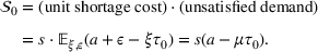
as the total supply, the shortfall demand can be expressed as
. Because the per unit shortage cost of the crop is
, the total shortage cost
incurred is
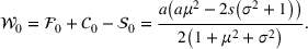
Net value. Net value
is the sum of farmer's and consumer's surpluses less the shortage cost incurred:
WHEN COST SUBSIDY
IS OFFERED
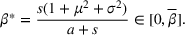
In the presence of a cost subsidy
, government will reimburse a fraction
of each farmer's total cultivation cost
, where
. Because the effective production cost is
, using (3), we can conclude that the farmer with cost
will grow the crop if and only if his average unit revenue is higher than his subsidized unit cost; that is,
where
is the fraction of farmers cultivating the crop. It is easy to observe from (8) that if cost subsidy is sufficiently high (i.e.,
), then all farmers will be enticed to cultivate the crop. In order to avoid such unrealistic cases wherein all farmers are enticed to cultivate the crop through cost subsidies, we restrict
to admissible values (we will revisit this in Assumption 3). Next, using the concept of rational expectation and (8), the fraction of farmers who sow the focused crop in equilibrium (which we denote by
), when a cost subsidy of
is offered, is obtained through the following result:
For any cost subsidy
, the fraction of farmers who cultivate the crop is
All farmers with cost
will grow the crop so that the fraction of farmers who grow the crop in equilibrium is
. Moreover, the threshold
(which is also the fraction of farmers cultivating the crop) is increasing in
(i.e.,
).
In order to focus on more pragmatic case of cost subsidies, we restrict
From Lemma 2, we can conclude that offering a high cost subsidy
will entice more farmers to cultivate the crop (because
). Additionally, Lemma 3 shows that enticing more farmers in the above manner through a high cost subsidy
will actually hurt farmer's surplus due to (i) supply glut of the crop and (ii) volatility in market prices. Enticing more farmers through a high cost subsidy increases the average production quantity of the crop, which decreases the crop's average market price thereby hurting farmer's surplus. Additionally, a high cost subsidy
that entices more farmers to cultivate the crop exposes them to price volatility due to yield uncertainty
thereby hurting farmer's surplus (also see Corollary 1). Hence, when
and
are high, then cost subsidies can hurt farmer's surplus.
The higher the values of average crop yield
or crop‐yield dispersion
, the lower is the viability of input cost subsidy in improving farmer's surplus (i.e., the smaller is the range of
values that can improve farmer's surplus). Furthermore, input cost subsidy does not increase farmer's surplus when either the average crop yield
or the crop‐yield dispersion
is sufficiently high so that
.
Even though cost subsidy may not improve farmer's surplus as discussed above, it always improves consumer's surplus through lower crop market prices (as shown in statement 2 of Lemma 3) and the increase in consumer's surplus outweighs the decrease in farmer's surplus, if any, so that the total surplus always increases (as shown in statement 4 of Lemma 3).
Net value of cost subsidy. By substituting (11)–(14) in (15), we can compute the net value
associated with cost subsidy
as
The following proposition provides the optimal cost subsidy
that maximizes the net value generated.
Let
where
is given in Lemma 1. The optimal admissible cost subsidy
that maximizes the net value
is
The corresponding crop production threshold is
and the optimal net value is
Although agricultural cost subsidy is more consumer‐centric and always improves consumer's surplus while a high subsidy could hurt farmer's surplus, as shown in Lemma 3, Proposition 1 shows that there exists a unique value of the subsidy (as given in (17)) that maximizes the net value generated. From (17), it is easily evident that a higher value of
) in order to offset the decrease in farmer's surplus due to (i) lower mean crop price (due to high
) and (ii) higher erratic crop price (due to high
). Lastly, the optimal net value increases in the crop's average yield
and decreases in the crop's yield variance
(i.e.,
and
), which indicates that between two crops with comparable cost and price structures, it is beneficial to offer cost subsidy to the crop with lower coefficient of variance.
We also analyze the second type of cost subsidy, which we term as additive cost subsidy, where each farmer who cultivates a crop is offered a fixed subsidy
. Through our analysis, we conclude that both multiplicative cost subsidy (that is discussed in the current section) and additive cost subsidy (that is discussed in Appendix B) result in the same optimal crop production
and net value
(that are given in Proposition 1). We refer the reader to Appendix B for further details about additive cost subsidy and its performance.
While a cost subsidy, being an input‐based subsidy, results in government sharing a fraction of farmers' cultivation costs thereby alleviating their financial burden, a crop's MSP is an “output‐based subsidy” that provides all farmers who cultivate the crop a minimum guaranteed crop price thereby protecting them from slumps in market price. Thus, MSP differs fundamentally from cost subsidy in its operationalization. Additionally, the fact that cost subsidy increases variability in market price (see Corollary 1), which acts against the governmental objective of protecting farmer's welfare, urges us to examine the impact of crop MSP in a detailed manner and compare its efficacy against that of crop subsidy: Can MSP offer high farmer's and consumer's surpluses and generate high net value? We examine this issue next.
WHEN CREDIT‐BASED MSP
IS OFFERED
We now consider the case when government offers a preannounced credit‐based MSP
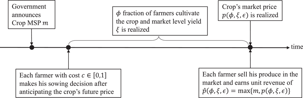
for the focused crop, which could influence the farmers' sowing decisions. The chronological sequence of events in the presence of MSP is illustrated in Figure 1. In the presence of such credit‐based MSP, farmers sow the crop if their average unit revenue from the crop is greater than their respective unit cost of cultivation. However, the expected revenue from the crop is determined by the precommitted MSP
of the crop along with the market price of the crop, which is realized after the crop's cultivation. The realized market price, in turn, is influenced by the quantity of the crop, as given in (1), while the latter is determined by the sowing decisions of the farmers. We capture all these dependencies in the analysis below.
Farmer cost and capacity model
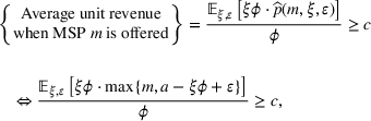
Under a credit‐based MSP scheme, when an MSP
is offered for a crop, a farmer who cultivates the crop is guaranteed a minimum revenue equal to
. In the event when the realized per unit crop price
to each farmer who grows the crop. However, if the realized price
is greater than
, then a farmer is entitled a revenue of
per unit of the crop and government incurs no expenditure. Therefore, a farmer who cultivates the focused crop earns a unit revenue of
at the time of selling the crop. Each farmer undertakes his sowing decision by anticipating the expected future unit revenue and weighing it against his production cost
is the proportion of farmers who choose to cultivate the crop. The following result shows that for any fraction
, MSP
reduces the variability in the revenue earned by the farmers who cultivate the crop.
For any
, MSP
reduces the variance of the revenue of a farmer who cultivates the crop.
The above result provides an inkling that MSP could potentially mitigate the variability in farmers' earnings, which we will revisit in Corollary 3 after characterizing the equilibrium in Theorem 1. Using the concept of rational expectation and (19), we obtain the fraction of farmers who sow the focused crop in equilibrium as follows:
For any
, which denotes the fraction of farmers who cultivate the crop, and any MSP
, let
There exists a unique threshold
that is the solution of
such that all farmers with unit production cost
will cultivate the crop and all those with
will not cultivate the cost, in equilibrium.10Moreover, the threshold
(which is also the fraction of farmers cultivating the crop) is increasing in
(i.e.,
).
It is important to note that
using the assumption that the crop price is nonnegative, so that
.
Next, as before, in order to avoid the unrealistic case that all farmers are enticed to grow the crop due to MSP, which is unusual in practice, we restrict
to the following admissible values:
, where
is the unique value that satisfies
(so that
).
The following result revisits the variability in unit revenue of farmers in equilibrium:
A higher MSP increases the variance in crop's production quantity. However, increasing
reduces the variance in the revenue earned by a farmer cultivating the crop if at least one of the following holds true:
The rate of increase in the crop production that is caused by
is sufficiently low.
is sufficiently high.
The yield and market potential variability (i.e.,
and
) are sufficiently low.
Although MSP
reduces the variability in the unit revenue for a fixed fraction of farmers who cultivate the crop (as shown in Lemma 4), this may not be true in equilibrium because, apart from offering a floor price,
affects the total crop production (by enticing more farmers to sow the crop as shown in Theorem 1), which amplifies the variability in the total crop production quantity that, in turn, increases the variability in the crop's price and so, in the unit crop revenues of farmers. Hence, care should be exercised to not entice too many farmers to cultivate the crop in order to contain the variability in per unit crop revenue. Next, it is intuitive that if
is very high, then it is very likely that the MSP is higher than the market price most often and hence the variability in the unit revenues of farmers reduces, as discussed in the second statement of the above corollary. Lastly, if the variability in yield and market potential is low, then the amplification in the variability of total crop production quantity as
increases is low, while the increased
offers a higher floor price to the farmers, which reduces the variability in per unit crop revenues. Thus, apart from the value of
, the distributions of
and
play a major role in determining if
increases or decreases the variability in farmer revenues. Now, in the next section, we explore the impact of
on the expected surpluses and the net value that it generates.
Performance metrics
For any given admissible MSP
, we compute the performance metrics—that is, farmer's surplus
The following result explains the impact of MSP on the performance metrics
,
,
, and
:
Farmer's surplus
, consumer's surplus
, and expenditure
are increasing in MSP
while the shortage cost
is decreasing in
.
Unlike input cost‐subsidy program that can hurt farmer's surplus when the subsidy is high, that is,
as shown in Lemma 3, a credit‐based MSP always improves farmer's surplus along with consumer's surplus, as shown in Lemma 5, because it insurers all farmers who cultivate the crop from low crop prices caused by crop's yield uncertainty.
Net value of MSP. The net value of MSP
is
Using the expressions for
,
,
, and
given above along with the base net value
given in (6), we obtain the following result:
The optimal MSP
that maximizes the net value
is the unique solution of the following equation11:
The corresponding crop production threshold is
, which is given in (16), and the optimal net value is
From (28) in Proposition 2 and (18), we can conclude that MSP generates the same optimal net value as a cost subsidy, that is,
. Hence, the question remains: Is MSP more beneficial than cost subsidy? In order to answer this question, we introduce the following result that compares the farmer's surplus that MSP provides against the surplus provided by cost subsidy.
The optimal MSP
offers higher farmer surplus than the optimal cost subsidy
while incurring a commensurately higher expenditure than cost subsidy (i.e.,
). Hence, administering optimal MSP
requires a higher budget than administering optimal cost subsidy
.
Proposition 3 proves that, even though MSP and cost subsidy offer the same optimal net value, MSP benefits farmers more than cost subsidies in terms of farmer's surplus. It also shows that MSP is efficient in transferring more value to farmers by commensurately increasing governmental expenditure without any loss of value.
By considering the results reported in Sections 5 and 6, we find that
MSP always improves both farmer's and consumer's surpluses. However, cost subsidy benefits consumers but it can hurt farmers cultivating the crop. This is because, although a cost subsidy reduces the deterministic input costs of the farmers, it exposes farmers to market price uncertainty and low market price.
Both MSP and cost subsidy improve the total surplus (i.e., the sum of farmer's and consumer's surpluses), and offer the same optimal net value (i.e.,
Although cost subsidy always increases the variance in unit revenues of the farmers, Corollary 3 reveals that MSPs can reduce the variability as long as they are properly set to not entice a huge number of farmers to cultivate the crop.
PROGRAM CHOICE UNDER BUDGET CONSTRAINT ON IMPLEMENTATION COST
In this section, we consider the case when policymakers are given a budget
and need to address the following question: Which of the two policies —MSP or cost subsidy—offers a higher net value? To answer this question, we solve the following two problems,
and
that correspond to cost‐subsidy and MSP programs, respectively (Table 1).
Comparing cost subsidy and MSP with respect to net value for an investment
The following result compares different performance metrics associated with both MSP and cost‐subsidy programs12:
By subsidizing the cultivation costs through cost subsidy, government will entice more farmers to cultivate the crop than MSP, at a given budget level
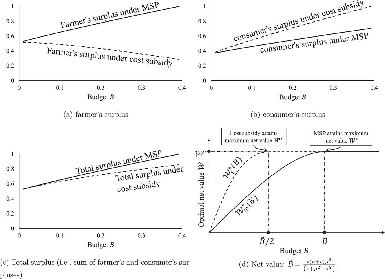
. This larger crop supply caused by cost subsidy will generate a higher consumer's surplus than MSP because cost subsidy substantially decreases the crop's market price. The consumer's surplus graphs are shown in Figure 2b. (The increased crop supply generated by cost subsidy will also reduce the shortage cost, as discussed in statement 4 of the proposition.)
Comparison between cost‐subsidy and MSP schemes
Despite higher consumer's surplus and lower shortage cost, cost subsidy can hurt farmer's surplus by exposing more farmers to lower and more variable market prices (as shown in Corollary 4 in Appendix C). On the contrary, MSP insulates all farmers who sow the crop from price falls through a floor price thereby improving the farmer's surplus greatly. Hence, statement 2 of the proposition reveals that cost subsidy will generate a lower farmer's surplus than MPS, as shown in Figure 2a. Furthermore, the lower market price that is due to the increased crop production triggered by MSP (as shown in Theorem 1) will, apart from increasing the consumer's surplus (as shown in Figure 2b), also increase the likelihood of farmers claiming the MSP. Therefore, government incurs a higher expenditure by offering MSP for a larger quantity of crop more frequently.
Finally, MSP offers higher farmer's surplus at higher expenditure as discussed above, but it also yields lower consumer's surplus and higher shortage cost. Hence, as statement 6 of the proposition reveals, MSP generates a lower net value than cost subsidy as shown in Figure 2d. (We provide the complete piecewise definition of
to operate with under a hybrid policy, the second statement (36) of the above proposition reveals that the combination of two programs does not create additional net value. In the absence of a budget constraint, a hybrid policy is unwarranted and a standalone cost‐subsidy program will suffice to maximize the net value generated. (Moreover, in the presence of a budget constraint, Proposition 7 in Appendix C proves a stronger result that a hybrid policy generates the same optimal net value as a standalone cost subsidy does, for any budget
. Therefore, using Propositions 4 and 7 (stated in Appendix C) we can conclude that, for any budget
, standalone cost subsidy alone suffices to maximize the net value that is generated.)
The above conclusion prompts us to raise the following important question: Do hybrid and MSP policies offer any additional benefit over cost subsidy? To explore this question, we first graphically illustrate the frontier of optimal hybrid policies, which we denote by
, in Figure 3. As shown in the figure, the optimal hybrid policies vary from optimal standalone cost subsidy (i.e., point
) to optimal standalone MSP (i.e., point
). We can easily show that farmer's surplus
and expenditure
increase at the same rate as we move from point
to
along the frontier (i.e., by increasing the MSP and decreasing the cost subsidy while retaining the resultant policy optimal), while consumer's surplus
and shortage cost
remain unchanged because the crop production is retained at
along the frontier, as shown in (34). This implies that the total surplus (i.e.,
) and net surplus (i.e.,
) also increase from
to
along the frontier. (We establish the technical details about the profile of
and other statements in Lemma 6 in Appendix C.) This observation enables us to “refine” the set of optimal policies for any budget
using the net surplus
to break the ties. Specifically, we define an efficient policy for a given budget
, which we denote by
, as follows:
That is, among all the hybrid policies that yield the maximum net value, the efficient policy
is the one that offers the highest net surplus. Therefore, using the fact that the net surplus is increasing along the frontier
from point
to point
in Figure 3, we can conclude that an efficient policy is unique and its expenditure is equal to
. Now, we introduce the following result that explains how the unique efficient policy can be implemented for any budget
.
Let
. For any budget
, we obtain:
If
is low, that is,
, then the efficient policy is to invest
in standalone cost subsidy (so that
).
If
is moderate, that is,
, then the efficient policy is to invest
in cost subsidy and
in MSP (so that
and
).
If
is high, that is,
, then the efficient policy is to invest
in standalone MSP (so that
) and retain
unused.
Optimal hybrid policies
Proposition 6 reveals that the actual choice of the efficient policy is solely driven by the amount of budget
that is available. Specifically, when
is moderate or high, the hybrid and standalone MSP policies offer the additional advantage of increasing the net surplus, without deteriorating the maximum net value.18
CONCLUSIONS
Our paper represents an initial attempt to examine the impact of a credit‐based MSP on farmers and consumers and compare its performance against a more common cost‐subsidy scheme.
We developed a stylized game‐theoretic model to evaluate the impact of cost subsidy and credit‐based MSP on (i) farmer's surplus, (ii) consumer's surplus, and (iii) the net value that the farmer‐support programs deliver. By assuming that farmers are infinitesimally small, rational, and strategic with heterogeneous crop production costs, we analyzed the impact of cost subsidy and MSP in the presence of market and crop production yield uncertainties and compared the performance of both the support schemes for any budgetary investment.
We found that, although optimal standalone MSP, hybrid (i.e., mixture of MSP and cost‐subsidy policies), and standalone cost‐subsidy policies all generate the same maximum net value, they are ranked in the decreasing order of their efficiency in achieving higher net surplus. However, the choice of the appropriate policy is determined by the availability of budget.
In addition to the factors that we discussed in the current paper, there are other aspects of MSPs to explore as future research. First, a natural extension of our work is to examine the performance of MSPs against cost subsidies when they are offered to multiple crops. It will be interesting to capture and understand the interaction between competing crops when farmers make the sowing decisions. Second, it is known that farmers tend to grow crops that are highly subsidized even though such crops are unsuitable to be grown in specific environmental conditions. This leads to adoption of unsustainable farming practices thereby resulting in depletion of natural resources. Examining such secondary impacts of agricultural subsidies, and how cost subsidies perform against MSPs to address the above environmental concerns, are both relevant and crucial. Third, given the complexity of the effects and interactions of various subsidy policies, policymakers often find it challenging to arrive at the efficient design of policies that should be offered and the optimal portfolio of crops for which the policies should be offered. Hence, addressing the large scale problem of multicrop MSPs, along with cost subsidies, is an interesting direction. The above are some problems pertaining to MSPs that are of high relevance and importance, especially in the context of emerging economies.
Footnotes
AGGREGATE MARKET‐LEVEL YIELD MODEL FOR DISCRETE NUMBER OF FARMERS
WHEN ADDITIVE COST SUBSIDY γ $\gamma$ IS OFFERED
AUXILIARY RESULTS
1
Besides MSPs, governments, NGOs, and a few firms in developing countries are also providing technical and scientific informational support to farmers when making cropping decisions (Chen & Tang, ). For instance, the Indian government had set up Krishi Vigyan Kendras (or Agriculture Knowledge Centers) that are run by the Indian Council of Agricultural Research, which provide necessary information and advice to farmers on farming. There are also many NGOs (such as Centre for Collective Development, Centre for Sustainable Agriculture, Krishiyodha, and others), mobile apps (such as AgriApp, Kisan Yojana, IFFCO Kisan, RML, and others), and companies (such as Ninjacart, KrishiHub, and others) that give inputs and assistance to farmers.
2
Many farmers in India often make their decisions based on the advice provided by the (risk‐neutral) advisory bodies.
3
In general, the cost of cultivating a crop can vary among farmers depending on the soil and natural resources locally available, the climatic conditions, and the farming practices they employ, which makes it imperative to consider cost heterogeneity when formulating a model.
4
We will defer the case of “partially correlated” yields to future research.
5
We adopt the standard Hotelling linear city for capturing the heterogeneous cultivation costs of the farmers (Tirole & Jean, ).
6
For tractability, we assume that every farmer “anticipates” the yields of all farmers (including his own) are “identically distributed” so that the ex ante average revenue earned by a farmer is the ratio of the total expected revenue earned by all the farmers who cultivate the crop to the number of farmers who cultivate the crop, as stated in ().
7
To explicate our analysis associated with the rational expectation concept, we analyze the case of
discrete farmers in Appendix A.
8
It is also obvious that if farmers are offered cost subsidy or MSP when
, then still all farmers will continue to grow the crop because they gain higher profit, thereby making the problem trivial.
9
It can be easily observed that offering more cost subsidies when all farmers are cultivating the crop always improves farmer's surplus because it is akin to offering free money; we avoid this trivial case that is of little practical relevance and focus on the more realistic case where not all farmers are enticed to cultivate the crop through cost subsidies, in order to capture the interactions between cropping decisions and farmer's surplus.
Here, although we discuss choosing between MSP and cost subsidy when exactly one of them has to be chosen, we will introduce hybrid policy in the next section where both MSP and cost subsidy can be implemented simultaneously.
13
Note that it suffices to consider the investment in the implementation cost because there exists a one‐to‐one correspondence between the implementation cost (i.e.,
) and the total cost (i.e.,
) via the equilibrium threshold (i.e.,
or
as the case may be). Hence, we can always check if the overall total budget constraint is satisfied for any budget invested in implementing the policy.
14
We define total surplus as the sum of farmer's and consumer's surpluses and net surplus as total surplus less the shortage cost; moreover, to recall, net value is net surplus less the expenditure.
15
We provide the mathematical expressions for net values generated by cost subsidy and MSP, for any given budget
, in Lemma in Appendix C.
16
We denote a hybrid policy that simultaneously offers cost subsidy
and MSP
by an ordered pair
.
17
We use the subscript “h” to denote hybrid policy.
18
We also provide a few supplementary results in Appendix C on how crop characteristics influence the efficient policy. We refrain from including them here because they are not the main focus of our discussion in the paper.
19
It is important to note that because the subsidy
is offered per unit input capacity that is invested by a farmer, who is infinitesimally small (i.e., his production alone cannot influence the market price), there is no scope for moral hazard. In other words, a farmer has no incentive to invest less than the input capacity that he holds and obtain the commensurately scaled input subsidy, so long as () holds true.
20
We use subscript
to denote additive cost subsidy.
ORCID
Prashant Chintapalli
Christopher S. Tang
References
1.
African Smallholder Farmers Group (ASFG) (2013). Supporting smallholder farmers in Africa. http://www.fao.org/family‐farming/detail/en/c/1109849/
2.
AkkayaD.BimpikisK.LeeH. (2021). Government interventions to promote agricultural innovation. Manufacturing & Service Operations Management, 23(2), 437–452.
3.
AlizamirS.IravaniF.MamaniH. (2018). An analysis of price vs. revenue protection: Government subsidies in the agriculture industry. Management Science, 65(1), 32–49.
4.
BardhanP.MookherjeeD. (2011). Subsidized farm input programs and agricultural performance: A farm‐level analysis of West Bengal's green revolution, 1982–1995. American Economic Journal: Applied Economics, 3(4), 186–214.
5.
BeraS. (2017). Madhya Pradesh launches new farm scheme to hedge price risks in farming. https://www.livemint.com/Politics/uDdclMv4VKUhGvpSEqtmqL/Madhya‐Pradesh‐launches‐new‐farm‐scheme‐to‐hedge‐price‐risks.html
6.
BrooksJ.WigginsS. (2010). The use of input subsidies in developing countries. In Global forum on agriculture (pp. 29–30), November 29–30. OECD Headquarters, Paris.
7.
ChandR. (2003). Minimum support price in agriculture: Changing requirements. Economic and Political Weekly, 38, 3027–3028.
8.
ChenY.‐J.TangC. S. (2015). The economic value of market information for farmers in developing economies. Production and Operations Management, 24(9), 1441–1452.
9.
ChibwanaC.FisherM.ShivelyG. (2012). Cropland allocation effects of agricultural input subsidies in malawi. World Development, 40(1), 124–133.
10.
ChintapalliP.TangC. S. (2020). The value and cost of crop minimum support price: Farmer and consumer welfare and implementation cost. Management Science, 67. https://doi.org/10.1287/mnsc.2020.3831
11.
DantwalaM. (1967). Incentives and disincentives in Indian agriculture. Indian Journal of Agricultural Economics, 22(2), 1.
12.
DeanV. W. (1996). Why not the Brannan plan?Agricultural History, 70(2), 268–282.
13.
FanS.GulatiA.ThoratS. (2008). Investment, subsidies, and pro‐poor growth in rural India. Agricultural Economics, 39(2), 163–170.
14.
FAO. (2020). India at a glance. http://www.fao.org/india/fao‐in‐india/india‐at‐a‐glance
15.
FoxK. A. (1956). The contribution of farm price support programs to general economic stability. In Policies to combat depression (pp. 295–356). NBER.
16.
GudaH.DawandeM.JanakiramanG.RajapaksheT. (2021). An economic analysis of agricultural support prices in developing economies. Production and Operations Management. https://ssrn.com/abstract=3103334
17.
HemmingD. J.ChirwaE. W.DorwardA.RuffheadH. J.HillR.OsbornJ.LangerL.HarmanL.AsaokaH.CoffeyC.PhillipsD. (2018). Agricultural input subsidies for improving productivity, farm income, consumer welfare and wider growth in low‐and lower‐middle‐income countries: A systematic review. Campbell Systematic Reviews, 14(1), 1–153.
18.
HuM.LiuY.WangW. (2017). Socially beneficial rationality: The value of strategic farmers, social entrepreneurs and for‐profit firms in crop planting decisions. Management Science, 65. https://doi.org/10.1287/mnsc.2018.3133
19.
HuangJ.LengM.ParlarM. (2013). Demand functions in decision modeling: A comprehensive survey and research directions. Decision Sciences, 44(3), 557–609.
20.
InnesR. (1990). Government target price intervention in economies with incomplete markets. Quarterly Journal of Economics, 105(4), 1035–1052.
21.
JayneT. S.RashidS. (2013). Input subsidy programs in sub‐Saharan Africa: A synthesis of recent evidence. Agricultural Economics, 44(6), 547–562.
22.
JayneT. S.SitkoN. J.MasonN. M.SkoleD. (2018). Input subsidy programs and climate smart agriculture: Current realities and future potential. In Climate Smart Agriculture (pp. 251–273). Springer, Cham.
23.
KazazB.WebsterS. (2011). The impact of yield‐dependent trading costs on pricing and production planning under supply uncertainty. Manufacturing & Service Operations Management, 13(3), 404–417.
24.
KrishnanV. B. (2018). What the agriculture census shows about land holdings in India. https://www.thehindu.com/sci‐tech/agriculture/indian‐farms‐getting‐smaller/article25113177.ece
25.
LiaoC.‐N.ChenY.‐J.TangC. S. (2017). Information provision policies for improving farmer welfare in developing countries: Heterogeneous farmers and market selection. Manufacturing & Service Operations Management, 21. https://doi.org/10.1287/msom.2016.0599
26.
LiaoC.‐N.ChenY.‐J.TangC. S. (2019). Information provision policies for improving farmer welfare in developing countries: Heterogeneous farmers and market selection. Manufacturing & Service Operations Management, 21(2), 254–270.
27.
MendelsonH.ParlaktürkA. K. (2008). Competitive customization. Manufacturing & Service Operations Management, 10(3), 377–390.
28.
MillsE. S. (1959). Uncertainty and price theory. Quarterly Journal of Economics, 73(1), 116–130.
29.
Ministry of Agriculture and Farmers Welfare, Government of India (2019). Categorisation of farmers. https://pib.gov.in
30.
NITI Aayog (2016). Evaluation study on efficacy of minimum support prices (MSP) on farmers. http://niti.gov.in/writereaddata/files/writereaddata/files/document_publication/MSP‐report.pdf
31.
PetruzziN. C.DadaM. (1999). Pricing and the newsvendor problem: A review with extensions. Operations Research, 47(2), 183–194.
32.
PrasadA. M. (2016). Subsidy reform: Seeding change through direct benefit transfer. https://indianexpress.com/article/india/india‐news‐india/subsidy‐reform‐seeding‐change‐through‐direct‐benefit‐transfer/
33.
RamaswamiB.SeshadriS.SubramanianK. V. (2018). The welfare economics of storage‐based price supports. Working Paper. https://doi.org/10.2139/ssrn.3262407
34.
SpitzeR. (1978). The food and agriculture act of 1977: Issues and decisions. American Journal of Agricultural Economics, 60(2), 225–235.
35.
SubbaraoD. (2011). The challenge of food inflation (Working Papers id:4594). eSocialSciences.
36.
TiroleJ.JeanT. (1988). The theory of industrial organization. MIT Press.
37.
TripathiA. K. (2013). Agricultural price policy, output, and farm profitability—Examining linkages during post‐reform period in India. Asian Journal of Agriculture and Development, 10(1), 91–111.
38.
XiaoS.ChenY.‐J.TangC. S. (2020). Knowledge sharing and learning among smallholders in developing economies: Implications, incentives, and reward mechanisms. Operations Research, 68(2), 435–452.
39.
XuZ.BurkeW. J.JayneT. S.GoverehJ. (2009). Do input subsidy programs “crowd in” or “crowd out” commercial market development? Modeling fertilizer demand in a two‐channel marketing system. Agricultural Economics, 40(1), 79–94.