
Abstract
Throughout the current COVID‐19 pandemic, governments have implemented a variety of containment measures, ranging from hoping for herd immunity (which is essentially no containment) to mandating complete lockdown. On the one hand, containment measures reduce lives lost by limiting the disease spread and controlling the load on the healthcare system. On the other hand, such measures slow down economic activity, leading to lost jobs, economic stall, and societal disturbances, such as protests, civil disobedience, and increases in domestic violence. Hence, determining the right set of containment measures is a key social, economic, and political decision for policymakers. In this paper, we provide a model for dynamically managing the level of disease containment measures over the course of a pandemic. We determine the timing and level of containment measures to minimize the impact of a pandemic on economic activity and lives lost, subject to healthcare capacity and stochastic disease evolution dynamics. On the basis of practical evidence, we examine two common classes of containment policies—dynamic and static—and we find that dynamic policies are particularly valuable when the rate of disease spread is low, recovery takes longer, and the healthcare capacity is limited. Our work reveals a fundamental relationship between the structure of Pareto‐efficient containment measures (in terms of lives lost and economic activity) and key disease and economic parameters such as disease infection rate, recovery rate, and healthcare capacity. We also analyze the impact of virus mutation and vaccination on containment decisions.
INTRODUCTION
The outbreak of the novel coronavirus disease (COVID‐19) in China in late December 2019 reminded us of the pandemics of recent history such as severe acute respiratory syndrome (SARS) and Middle East Respiratory Syndrome. Even though each pandemic has its own severity, mortality rate, and other specific disease characteristics, they share some similar economic consequences. At the time of writing this article, the number of people who have lost their lives worldwide due to the COVID‐19 pandemic has exceeded 4,200,000, 1 the number of jobs lost in the United States has reached 22,200,000, 2 and expected GDP growth has been reduced by 10% in the United States and 12% in Europe (Gormsen & Koijen, 2020). Pandemics are far more than a health crisis; they also have significant economic and societal impacts.
Containing the spread of pandemics such as SARS and COVID‐19 is a major challenge for governments due to economic, social, and political factors. During the COVID‐19 pandemic, we have witnessed a wide range of containment measures. Some countries, such as Sweden, opted for a strategy of attempting to acquire herd immunity and adopted minimal containment measures. Other countries enacted strict containment measures, from imposing social distancing rules, closing schools and shopping malls, canceling arts and culture events, and closing borders to enforcing national lockdowns, curfews, and quarantines. The overarching goal of these measures is to slow the spread of the disease and flatten the pandemic's curve to bring it below the threshold of healthcare capacity. As illustrated in Figure 1, if the number of actively infected individuals exceeds the capacity of hospitals and clinical organizations at any given time, the quality of healthcare services will quickly degrade, leading to a significant increase in the number of deaths.
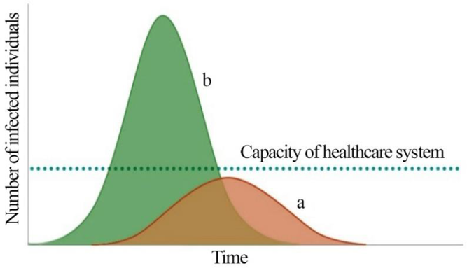
Two scenarios for the spread of pandemics with (a) and without (b) containment measures
While imposing severe containment measures (e.g., curfews, large‐scale social distancing, quarantine, and lockdowns) may limit the spread of the pandemic (as in the case of Australia) and decrease stress on the healthcare system, yet such severe measures may derail the economy by disrupting supply networks, manufacturing lines, and household demand for goods and services, leading to lost jobs, economic stall, and social disturbances. On the other hand, under mild or no containment measures, such as depending on herd immunity, the economic implications of the pandemic may be limited but the capacity of the healthcare system would be quickly exhausted, possibly leading to a significant amount of lives lost. Hence, when determining the severity of containment measures, governments face a stark trade‐off between maintaining economic activity and reducing lives lost. In this study, we examine this trade‐off by providing a multiobjective decision model that incorporates both the economic and health implications of containment measures into the decision maker's objective function.
Finding an appropriate containment policy is further complicated due to the unpredictable nature of disease spread and the impact of a government's other mediating actions during a pandemic. For example, the effectiveness of containment measures on the rate of disease spread can be uncertain due to unpredictable social reactions to the measures, possible virus mutation, and potential vaccination and treatment development. Economic stimulus packages and short‐term investments into healthcare may also condition the impact of government containment measures on economic activity and lives lost. Finally, the impact of measures may also be moderated by the level of economic and containment measures taken by the rest of the world, because a global economic slowdown will eventually affect local economies. Our model aims to incorporate these relevant problem dynamics into a unified decision‐making framework for governments.
Given the duration of a typical pandemic (2–3 years), we track the economic impact of the disease through the change in the industrial production (IP) index, 3 which is a good proxy for change in gross domestic product (GDP). Estimating the sensitivities of the economic activity level and disease spread to the strictness (level) of containment measures is a key driver of our decision model. Hence, in Section 5, we provide two empirical models to estimate those sensitivities. We use University of Oxford's (2020) country‐level containment reports for tracking the level of containment measures and calculate the disease spread again at the country level using publicly reported case numbers. University of Oxford reports an aggregate containment level for countries, which can be scaled between 0 and 1, where 0 means no containment effort and 1 means complete lockdown. The details of the empirical models used for estimating the input parameters are provided in Section 5.
In this paper, we develop a stochastic multiobjective dynamic program to determine the level and timing of government interventions during a pandemic. The dual objectives of the hypothetical government are to (i) minimize the impact of containment measures on economic activity (measured as change in IP) and (ii) minimize the expected number of lives lost during the pandemic, subject to the stochastic evolution dynamics of the disease over time and the capacity of the healthcare system. Motivated by real‐life containment activities, we focus on deriving and analyzing two common classes of control policies: (i) static containment policies, where the level of containment measures remains mostly fixed throughout the planning horizon, and (ii) dynamic/flexible containment policies, where the level of containment measures is revised based on the evolution of disease spread over time. For example, the herd immunity approach in Sweden and the full lockdown in China during the early phases of the pandemic can be classified as examples of static containment policies. It is also possible to consider static containment policies, where the containment level is raised to a specific threshold between no containment and full lockdown, and is kept fixed throughout the planning horizon. Dynamic containment policies are also commonly used in practice. For example, the United Kingdom started with a low level of containment by imposing loose social distancing rules in early April 2020, then, as infections increased, it raised the containment level by imposing additional measures, and finally, in September 2020, the country moved to a full lockdown for 2 weeks. When cases decreased by early winter, they eased the lockdown restrictions.
Although it is intuitive that dynamic containment policies would perform better than static policies due to their flexibility in responding to a pandemic's evolution, it is not a priori evident whether these benefits are significant enough to justify the switching costs associated with frequently updating containment measures. Frequently updating containment measures are not desirable as they are subject to significant tangible and intangible economic, social, and political costs. In addition to the deadweight economic losses due to opening and closing businesses, frequently changing the level of containment during the pandemic creates economic and social uncertainty, which may lead to prolonged labor disturbances and social instability. In this paper, we focus on the quantifiable benefits of dynamic policies (over static policies), which can be compared to the costs of implementing such complex rules in practice.
We contribute to the literature with the following main points: We provide a decision‐support framework for policymakers by integrating disease‐spread models with stochastic dynamic optimization techniques. Unlike the existing research on pandemic disease control, we examine the broader problem of managing a government's level of containment measures to prevent the spread of a pandemic while minimizing the effect of such measures on economic activity and lives lost. Our model reflects the decision maker's ability to revise containment measures as the disease evolves over time. Our framework enables us to characterize a Pareto‐efficient set of containment policies that are undominated in terms of lives lost and level of economic activity. Through a comprehensive set of sensitivity analyses, we examine the impact of healthcare capacity and disease characteristics on containment decisions. We find that under the Pareto‐optimal set of containment policies, multiple peaks in the pandemic are likely to occur unless when the disease spread rate is high and the recovery period is long. In addition, targeting a high level of economic activity typically generates fewer but steeper peaks in the pandemic. We compare static and dynamic containment policies and observe that the dynamic policies are most beneficial when the disease spread is low and recovery takes longer. Further, governments targeting a moderate level of economic activity benefit more from dynamic policies. In addition, a close examination of the Pareto‐optimal set of containment policies reveals a key insight: Under low or high levels of containment measures, lives lost are highly sensitive to target economic activity level. Under intermediate levels of containment measures, however, changes in target economic activity level do not significantly affect lives lost. Finally, we also analyze the impacts of possible vaccination and virus mutation on the Pareto‐optimal set of containment measures and disease spread. We find that under a relatively low level of target economic activity, starting vaccinations after 9 months effectively flatten the peaks in a pandemic. If vaccinations are delayed, the benefits in terms of reduced lives lost quickly decrease. We also observe that the effectiveness of vaccination programs (in terms of reduced lives lost) is significantly compromised under high levels of target economic activity. Virus mutation has a qualitatively similar, but opposite, effect on the results.
The rest of the paper is structured as follows: We provide a review of the related literature in Section 2, followed by a description of our time‐dependent disease spread model in Section 3, and the decision model in Section 4. In Section 5, we discuss the estimation of the model parameters, and we devote Section 6 to the analysis of the model. We conclude with discussions and future research directions in Section 7. In addition, in Supporting Information Appendices A and B, we discuss extending our results under vaccination and virus mutation scenarios. Finally, we provide the details of our empirical analysis in Supporting Information Appendix C.
LITERATURE REVIEW
In the literature, there is an extensive amount of research on modeling pandemic‐spread dynamics using approaches that range from deterministic models (e.g., Albi et al., 2021; Chen et al., 2016; Sene, 2020) to stochastic models, such as discrete event simulation and system dynamics (Ghaffarzadegan & Rahmandad, 2020; Xie, 2020), to hybrid models (Ardabili et al., 2020; Funk et al., 2018). However, there is limited work linking outbreak dynamics to decision‐support models. With a few notable exceptions (Boloori & Saghafian, 2020; Eryarsoy et al., 2022), the relevant literature mostly focuses on analyzing pandemic spread.
Recently, a number of studies have been published exploring different types of containment measures to control the spread of a pandemic. Many of these studies examine the impact of a particular containment action—such as air traffic restrictions (Zlojutro et al., 2019), complete lockdown (Singh & Adhikari, 2020), and social distancing (Qiu et al., 2020; Thunström et al., 2020)—on the disease spread. Having focused on the COVID‐19 case, a comprehensive study by Ferguson et al. (2020) evaluates the impact of nonpharmaceutical interventions, including case isolation at home, voluntary home quarantine, social distancing of elderly people, closures of schools and universities, and general‐population social distancing. The authors conclude that to significantly reduce contact rates, multiple interventions need to be integrated. Giordano et al. (2020) suggest a forecasting model based on a modified version of Kermack–McKendrick's susceptible, infected, recovered (SIR) model to plan effective pandemic control. Using a compartmental model, the authors discriminate between diagnosed and undiagnosed patients and run scenario analyses for implementing countermeasures. Similar to Ferguson et al. (2020), their findings reveal that multiple intervention policies, such as widespread testing, contact tracing, and social distancing, should be integrated to end the outbreak. The literature also considers the impact of mobility patterns (Delen et al., 2020), age‐specific contact settings (Kyrychko et al., 2020), as well as popular discontent and social fatigue on pandemic control policies (Ouardighi et al., 2021).
A few recent works examine the economic impact of intervention policies for COVID‐19. For instance, Boloori and Saghafian (2020) provide an analytical decision‐making framework based on a compartmental disease‐spread model to study the economic burdens of pandemic containment policies in the United States. They suggest that while severe societal intervention policies may not be cost effective, the policies imposed by the US government over a 4‐month period increased quality‐adjusted life years per capita. In another attempt, Eryarsoy et al. (2022) develop deterministic mathematical formulations to study the economic impact of government interventions. The authors develop a multistart variable neighborhood search algorithm to suggest intervention strategies for policymakers. Their findings reveal that when disease severity is low and the estimated economic burden of pandemic containment policies is high, the policymaker should not engage in any intervention policy.
The societal value placed on lowering the statistical likelihood of one death is referred to as the value of statistical life (VSL) (Viscusi & Aldy, 2003). While various methods of fixing a monetary value for a human life have already been suggested by different protagonists, pandemics forced the globe to confront yet another unsettling trade‐off between human life/misery and economic gain. Within labor‐market studies, a sizable body of research has emerged that estimates VSL (Mrozek & Taylor, 2002). In healthcare operations, this issue is usually addressed from the “efficiency” point of view (Harris, 1987). As a result, to enable comparisons across different areas of healthcare, standard measures of health outcome, such as the quality‐adjusted life years (QALY) (Zeckhauser & Shepard, 1976) and disability‐adjusted life years (DALY) (Murray, 1994), were suggested. While the debate on the theoretical underpinnings and practical implications of those measures are still ongoing, the common overarching goal is to identify a healthcare strategy that results in a minimal cost per QALY or DALY (Whitehead & Ali, 2010). When considering a particular treatment for a particular illness, such as a cardiovascular disease or diabetes mellitus, QALY and DALY provide good measures of the cost‐effectiveness of a treatment in terms of allocating financial resources. In a pandemic context, however, the number of lives lost provides an easier and direct way of measuring the effectiveness of containment policies. Hence, we focus on the number of lives lost as one of the governmental objectives in our context.
In this study, we aim to provide a decision support framework for policymakers by integrating disease‐spread models with dynamic optimization models. Unlike the existing research, we examine the broader problem of optimizing a government's level of containment measures to prevent the spread of a pandemic while considering the dual objectives of minimizing lives lost and maximizing level of economic activity. Our analysis uncovers the connection between these two critical objectives by providing a Pareto‐optimal set (efficient frontier) of containment policies. Hence, our multiobjective approach is a generalization of the constrained optimization models, which minimize lives lost (or maximize QALY) under a given level of economic activity or budget constraint. Moreover, we estimate the model parameters through a comprehensive empirical analysis, which provides strong practical implications. We numerically illustrate the impact of healthcare capacity and other mediating factors on the trade‐off between lives lost and economic activity during a pandemic. We also identify the factors that drive multiple peaks in a pandemic under the Pareto‐optimal set of policies.
PANDEMIC MODEL
In the literature, there are several approaches for modeling disease spread. Perhaps the simplest and most well known is Kermack–McKendrick model, also known as the SIR model. SIR is a Markov model that has been used to explain the fast increase and decrease in the number of infected individuals in many pandemics. The SIR and its variants (such as susceptible‐infected‐susceptible (SIS), and susceptible‐exposed‐infectious‐recovered (SEIR)) generally fall under deterministic compartment models, and have been widely used to analyze the spread of pandemic diseases (Keeling & Rohani, 2011; Wearing et al., 2005; Wu et al., 2020). These models are represented by a set of differential equations, where various disease‐specific parameters describe the growth rates of disease among population compartments (Hethcote, 2000).
As illustrated in Figure 2, in this study we use a modified version of the SIR model. Our susceptible‐infected‐recovered‐deceased (SIRD) model consists of four compartments (or states) and three parameters, where the transition between states is indicated by arrows. The state variables


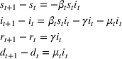
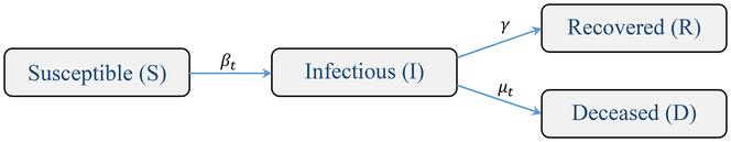
The time‐varying SIRD framework and its parameters
We note that in the medium and long term, a government's healthcare‐related measures (such as investing in drug and treatment development as well as increasing ICU capacity) may affect the recovery rate


It is worth noting that the SEIR model (with state variables Susceptible, Exposed but not infectious (E), Infectious, and Recovered) may also be used to model the spread of COVID‐19 because there is a period where the infected individual does not show any symptoms but is capable of infecting others. Having a very similar structure to SIRD, the SEIR model consists of only one additional parameter,

OPTIMIZATION MODEL
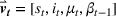
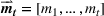
In this section, we provide a multi‐period discrete‐time optimal control problem to determine the level and timing of a government's containment measures during a pandemic. We use discrete weekly intervals both for modeling disease spread and making containment decisions. In each decision period


Higher values of


Notation for the mathematical model
The variable cIP denotes the significant control variables of the empirical estimation model used to estimate the relationship between the IP index and containment measures in Section 5.1.
Mathematical formulation
We assume that the government has two objectives without any a priori preference for one of them. The first objective is to minimize the impact of containment measures on economic activity, as defined in the following: Minimize the impact of containment measures on expected level of economic activity (i.e., maximize the expected level of economic activity)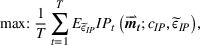
where the function Minimize the total number of expected lives lost


where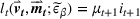
The function 


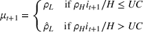
In addition to the inherent disease characteristics, utilization of the healthcare system affects the quality of treatment and the death rate, 


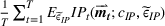
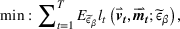
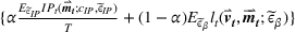
We use the scalarization method to represent our multiobjective, multiperiod stochastic dynamic program. Scalarizing a multiobjective problem means formulating a single‐objective version of the problem using a scalar 


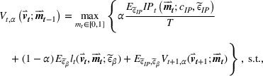


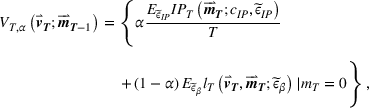
At time 


Together with the initial conditions in Equation (7), Equations (8)–(12) describe the modified time‐varying SIRD model for the spread of the disease over time (i.e., 


The model in (6)–(14) is a high‐dimensional dynamic program with a nonconvex feasible region. 7 As a result, even when we discretize the problem with monthly decision epochs, the model is still computationally intractable given that a pandemic may last for more than 1 year. Therefore, we continue with a weekly model to update disease evolution and containment measures and resort to heuristic containment policies. Next, we explain our parameter estimations for our model.
PARAMETER ESTIMATION
In this section, we provide a brief empirical analysis to determine the sensitivities of the economic activity level 


Estimating the impact of containment measures on economic activity
During the COVID‐19 outbreak, evaluating the impact of a government's containment measures on economic activity has been challenging due to the short time span of the evaluation period combined with the low dissemination frequency of the main macroeconomic variables. In order to examine the impact of governments’ containment measures on economic activity, we first set our sample country selection to G20 members. According to the International Monetary Fund (IMF), G20 countries account for 80% of global economic productivity, and therefore are considered a good representative of the world's total production output. However, since the European Union (EU) is counted in the G20, together with its largest economies of Germany, France, the United Kingdom, and Italy, we remove the EU from our sample set. Further, another member, Saudi Arabia, prefers not to disclose its various statistics on macroeconomy and international trade. Therefore, we also exclude it from our analysis.
Change in level of economic activity is commonly measured by change in GDP. However, in our case, GDP cannot be taken as the dependent variable, because due to its quarterly announcement frequency it gives us an exceedingly small sample to make a robust inference about statistical analysis. Moreover, initial GDP announcements are usually revised multiple times throughout the year, making them even more questionable to use in our analysis.
As a higher frequency proxy for GDP, we take the seasonally adjusted IP index, which is announced on a monthly basis. One of the main reasons why IP is a good proxy for GDP is that value added by IP represents a substantial share of GDP, especially for big economies such as G20 members (see NBER's Business Cycle Dating Committee 8 ; Rünstler & Sédillot, 2003). However, some G20 members do not disclose their IP values or stopped disclosing them some time ago. These countries are Australia, Argentina, India, Indonesia, Mexico, and South Africa, and so we exclude them from our sample country set. Eventually, we end up with 12 countries: the United States (1), China (2), Japan (3), Germany (4), the United Kingdom (6), France (7), Italy (8), Brazil (9), Canada (10), Russia (11), Korea (12), and Turkey (19), where the numbers in the parentheses denote the countries’ positions in the nominal GDP ranking in the world at the end of year 2019 by IMF estimates. The resulting country sample accounts for more than 65% of global GDP in the same year. 9 The details of the empirical analysis and data are provided in Appendix C in the Supporting Information.
Dependent variable
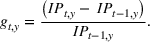
The monthly IP values cover from the end of December 2019 till the end of May 2020 (June 2020) for Brazil, Canada, Germany, France, the United Kingdom, Italy, Russia, and Turkey (for China, Japan, Korea, and the United States). Since we consider the monthly changes in IP values as the dependent variable, we end up with 64 country × month observations in an unbalanced panel data format. Accordingly, our dependent variable

Main independent variable
In our setup, the independent variable of special interest is a government's level of containment measures. Suppose that the independent variable 


This index is weekly updated, whereas our IP variable is a monthly indicator. Therefore, we synchronize these two datasets by taking only the monthly changes in Oxford's index. In our empirical analysis, we consider the monthly level change (index‐level difference between two consecutive months) as the key independent variable:
However, since measures taken by a government in the previous period can also affect the current period's IP, we include both the current (

Control variables
We also included a number of control variables that would likely condition the impact of a government's containment measures on economic activity. In particular, we included the monthly change in the variables described in Table 2. 10
Explanation of control variables
Model and results
We estimate the following model in the form of an unbalanced panel regression to measure the impact of government containment and closure actions: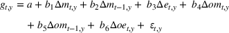
To have a robust framework, we use three alternative panel regression models, namely (i) pooled estimation, (ii) fixed‐effect estimation, and (iii) random effects (generalized least square) estimation, where standard errors are heteroscedasticity and autocorrelation robust. We observe that the model performs a fairly good fit to the data with an R
2 value around 0.50 for all estimation methods. Both quantitative and qualitative results are similar across the alternative estimation techniques, and therefore we interpret the economic findings based on the pooled regression results provided in Table 3. We observe that 


Pooled estimation results for the impact of containment measures on economic activity
R 2 = 0.501
On the basis of our empirical analysis, we use the significant variables and their coefficients in Table 3 to describe the relationship between containment measures and the level of IP index, that is, given 


Estimating the sensitivity of containment measures on disease spread
In this part, we examine the effect of a government's level of containment measures on the infection rate of the disease, that is, we estimate 


In our setup, both 


For robustness, we use three alternative models, namely (i) pooled estimation, (ii) fixed‐effect estimation, and (iii) random effects (generalized least square) estimation. Since all models yield similar results, we only report the coefficients obtained via pooled estimation.
According to the estimation results, the current and past 4 weeks’ containment measures taken by a government can significantly reduce the disease infection rate in that country, which confirms our earlier expectations. Table 4 also shows that the impact of containment measures on infection rate is gradually recognized over time. Based on our empirical analysis, we use the significant variables and their coefficients in Table 4 to describe the relationship between containment measures and the change in disease spread, that is, 
Pooled estimation results for the impact of containment measures on disease spread
R 2 = 0.0201
SIRD model estimates and numerical setup
Our disease‐spread model includes two key parameters: recovery rate 


Regarding the base infection rate 


For COVID‐19, the hospitalized fraction of individuals 


ANALYSIS: CONTAINMENT POLICIES
The high dimensionality and nonconvexity of the dynamic program in Equations (6)–(14) render it impossible to optimally solve real‐sized problems. Therefore, motivated by our practical observations, we focus on two common classes of control policies: (i) static containment policies and (ii) dynamic containment policies. We use the infectious ratio, 


Static containment policies
Static containment policies may be desirable by governments due to their simplicity and the provided certainty about planning future social and economic activities. Canceling work meetings and travel plans in response to a change in containment measures would have both economic and social consequences. Similarly, frequently opening and closing a business, as a result of changes in containment levels, may result in deadweight hiring and layoff costs. Similar deadweight losses also apply when negotiating rents and financial contracts in the markets. In addition, from a societal point of view, uncertainty associated with containment measures may lead to social disturbances and instability. In this sense, implementing a static containment policy provides individuals and businesses with more certainty about the level of containment measures, enabling them to avoid deadweight social and economic costs due to cancellations and updates, but these policies have limited flexibility to respond to the evolution of the pandemic.
During the COVID‐19 pandemic, we have observed examples of static policies in China and Sweden. China triggered a full containment policy in Wuhan soon after infection numbers reached a certain threshold and kept those strict containment measures in place until the infection numbers significantly decreased. Sweden adopted a static policy to the other extreme. After infection numbers reached a certain level in the country, they initiated loose voluntary social distancing and mask use and they have mostly kept these measures fixed throughout the pandemic.
The generalized version of the static policies discussed above is given in Equation (19). Here, 


In practice, it is not possible to initiate a containment measure as soon as the first person gets infected by a disease. It takes a certain amount of time and effort for governments to detect and verify the significance of an infection and for the World Health Organization to determine the importance and severity of the situation. On the basis of COVID‐19 experience, we will take this threshold to be 


Feasible and Pareto‐efficient static policies with minimum intervention trigger

In Figure 3, each point corresponds to a particular static policy identified by the pair of containment level and policy trigger (


The shape of the efficient frontier in Figure 3 reveals an important relationship (which also persists under the dynamic policies) between the level of economic activity and lives lost during the pandemic. For low and high levels of IP index, the number of lives lost is highly sensitive to changes in economic activity, whereas this sensitivity decreases under intermediate levels of IP index. For example, increasing the level of economic activity from 75% to 80% results in 78 additional lives lost, whereas increasing economic activity from 80% to 85% results in fewer than 35 additional lives lost. A close examination of this result together with the structure of containment policies on the efficient frontier reveals a key managerial insight: Under low or high economic activity targets, containment has a marginal impact on economic activity but has a significant influence on lives lost. However, when economic activity targets are set at intermediate levels, the number of lives lost becomes less sensitive to variations in containment level.
Static policies are desirable due to their stable nature and predictability in practice. However, they lack the flexibility to react to changes in infection numbers. Next, we discuss another class of common policies, which dynamically revises containment level based on disease spread, and compare it with static policies.
Dynamic containment policies: Band control policies
Band‐type dynamic containment policies are commonly used by governments. In this case, when the infectious ratio 

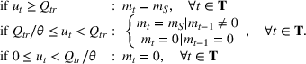
In practice, most governments’ dynamic policies resemble single‐ and double‐band policies, and hence we only focus on such policies. Equation (20) formalizes a single‐band control policy, and Figure 4 provides a visual illustration of it for the base‐case parameters:
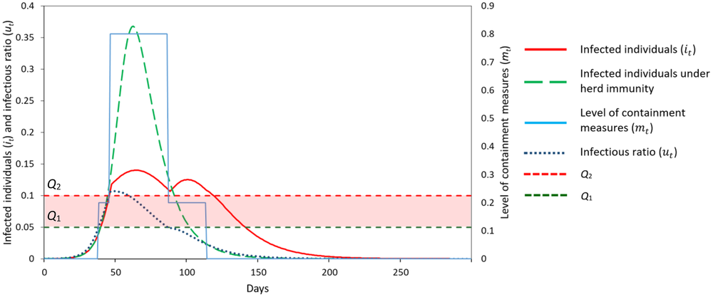
Illustration of a single‐band policy
The single‐band policy is described by a control band (


Figure 4 illustrates implementing an arbitrary single‐band policy with parameters (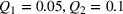
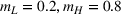


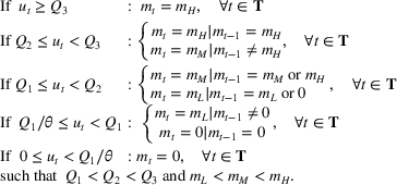
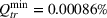
Figure 5 depicts implementing an arbitrary double‐band policy with parameters (


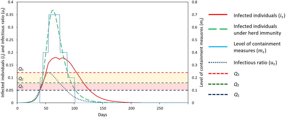
Illustration of a double‐band policy
Figure 6 illustrates the Pareto‐efficient set of static and dynamic policies under our base‐case parameter setting, where the upper, middle, and lower lines represent Pareto‐efficient double‐band, single‐band, and static policies, respectively. We observe that there can be a significant gap between the performance of static and dynamic policies. Moreover, double‐band policies outperform single‐band policies as well. After two bands, considering more control bands has little value in our model, and hence we focus on double‐band policies for the rest of our numerical analysis when referring to dynamic containment policies.
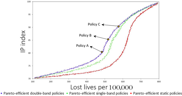
Pareto‐efficient set of static, single‐, and double‐band policies Note: In our numerical illustrations, we report infection numbers and infectious ratios with daily intervals for better granularity
In Figure 7, we examine the performance of three Pareto‐efficient double‐band containment policies such that the level of economic activity corresponds to 80% (policy A), 85% (policy B), and 90% (policy C). Figure 7a shows the performance of policy A, which generates 483.5 lives lost per 100,000 individuals. The policy results in two peaks in the pandemic. It initiates a low level of intervention at the beginning of the pandemic, followed by a strict containment after day 56; once the infectious ratio decreases substantially around day 203, the policy decreases the containment level, and the number of active cases starts to increase again, resulting in a second peak around day 301, followed by another short period of strict containment. After day 385, the government decreases the containment level again and keeps it low until the pandemic almost ends after day 700.
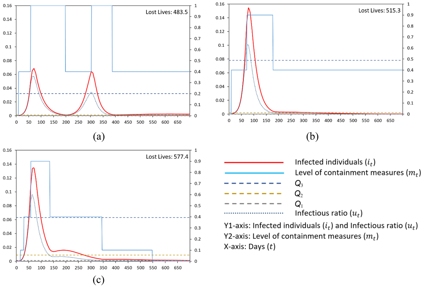
Containment measures and infected individuals over time under the Pareto‐efficient double‐band policies with IP index = (a) 80%, policy A; (b) 85%, policy B; and (c) 90%, policy C. Note: In Figure 7a,b, the threshold Q1 is too low to be observed visually
Policy B on the efficient frontier results in an economic activity level of 85% and 515.3 lives lost per 100,000 individuals. In this case, the policy reacts less aggressively to the spread of the pandemic, that is, the decision maker waits longer to initiate a high level of containment, and the level is kept high for a shorter period of time. As a result, we observe a single but steeper peak in the pandemic.
When we move to point C on the efficient frontier, the level of economic activity increases to 90% and lives lost per 100,000 individuals increase to 577.4. In this case, as compared to policy B, the government initiates a high containment level earlier but keeps it for a shorter period, resulting in a slightly lower pandemic peak with a fatter and longer tail. These actions result in a higher level of economic activity at the expense of more lost lives.
When we compare policies A and C on the efficient frontier of the double‐band containment policies, we observe that a 10‐point increase in economic activity from 80% to 90% results in a 19.42% increase in lives lost under our base‐case parameter settings. This trade‐off, however, naturally depends on the level of healthcare capacity and the rate of increase in lives lost when healthcare capacity is saturated, as measured by 
Absolute and percentage change in lives lost on the efficient frontier when the level of economic activity increases from 80% to 90% for varying levels of 


To increase the level of economic activity, the government implements milder containment measures, which leads to more lives lost. As healthcare capacity increases, lives lost due to capacity saturation decreases, leading to a relatively lower death toll due to increased economic activity on the efficient frontier. Similarly, increasing the ratio 
Impact of disease parameters on Pareto‐efficient policies
In this section, we examine the performance of Pareto‐efficient solutions under a varying base infection rate (

In Figure 8, we consider the Pareto‐efficient dynamic policies that achieve an 80% economic activity level.
14
Our base‐case corresponds to the setting with 


Impact of base infection rate

Figure 9 presents the same set of results for the Pareto‐efficient dynamic policies that achieve a 90% economic activity level, that is, when the government targets a higher level of economic activity as compared to Figure 8. The results are qualitatively the same as the case in Figure 8, except that now we observe the government implements weak containment policies leading to fewer but steeper peaks in the pandemic. We repeated our analysis with other levels of economic activity and found that the insights above are robust with respect to the level of economic activity.

Impact of base infection rate

Value of dynamic policies
In this section, we present the value of dynamic policies as compared to static policies under the Pareto‐efficient set of decisions (Figure 10). In particular, for a given level of economic activity, we compare the minimum lives lost under dynamic and static policies. This analysis helps to enclose the economic and operational parameters under which dynamic policies provide significant gains (in terms of reduced lives lost) over static approaches. On the efficient frontier, we define the benefit of dynamic policy as: (

Value of dynamic policy for varying levels of economic activity, base infection rate

We observe that the value of dynamic policies is highest when the level of economic activity is neither too high nor too low. This is because, under very high or low economic activity targets, there is little room for updating containment levels in response to changes in disease spread. We observe that the maximum benefit from a dynamic policy is obtained under low infection rate 

CONCLUSION
During a pandemic, governments face a key trade‐off when imposing containment measures. Such measures can be effective in reducing disease spread and the load on the healthcare system, but they can also cause economic stall and social and political unrest, indirectly leading to reduced quality of life for the population. In this study, we examine this trade‐off by providing a multiobjective decision model that incorporates both the economic and health implications of containment measures into a decision maker's objective function. We hope that our analysis will provide decision makers with valuable insights about when and how to implement containment measures during a pandemic.
We develop a decision‐support framework for policymakers to determine the level of containment measures during a pandemic by integrating disease spread models with stochastic dynamic optimization models. We identify the Pareto‐efficient set of containment policies under two common classes of control policies, namely static and dynamic. In general, as the recovery gets faster or the infection rate decreases, we observe more frequent but less steep peaks in the pandemic as the containment measures prove to be very effective in controlling the disease spread. However, when recovery is slow and the infection rate is high, then we typically observe a single steep peak because managing the spread of the disease with containment measures becomes very difficult. In addition, targeting a high level of economic activity is also likely to generate fewer but higher peaks in the pandemic.
The shape of the efficient frontier also reveals a key managerial insight about the sensitivity of governmental objectives to containment measures: Under low or high containment levels, the marginal impact of containment is low on economic activity but high on lives lost. However, for intermediate levels of containment measures, our results suggest that increasing (decreasing) containment level quickly reduces (increases) economic activity while resulting in little reduction (increase) in lives lost.
We also compare the performance of static and dynamic containment policies on the efficient frontier. We find that under very high or low economic activity targets, there is little room for updating containment levels in response to changes in disease spread, and hence there is little gain in using dynamic containment policies. Dynamic policies are particularly valuable when the disease parameters are likely to generate multiple peaks under a target economic activity level.
Our work can be extended in several directions. One possible extension could be considering an open population. Unlike the main assumption in the basic SIRD model, rather than requiring a closed population, one may include the possibility of incoming passengers through open and/or semiopen borders in the model. As another future work, an analysis could be conducted to incorporate the number of lives lost due to reduced economic activity and jobs lost driven by strict containment measures. Also, modeling uncertain vaccination effectiveness due to emerging new virus strains may be an interesting extension.
In addition to imposing disease containment measures to slow down disease spread, investing in healthcare capacity is an important dimension of pandemic management. In this study, we treat the healthcare capacity as a constant over time. While it is difficult to expand ICU capacity overnight, in medium and long term, acute care beds may be converted to ICUs or additional ICUs can be created. During the pandemic, governments have strived to increase healthcare capacity either by building new and temporary hospitals (Lardieri, 2020; Zhu et al., 2020) or by converting acute care beds to ICUs (Panico, 2020) to meet the increasing demand for healthcare resources. A promising future research direction would be to consider integrating disease containment measures with healthcare capacity expansion decisions to improve the effectiveness of pandemic management.
Footnotes
1
https://www.worldometers.info/coronavirus/.
2
https://www.reuters.com/article/us‐usa‐economy‐idUSKBN29D0J9.
3
The IP index is available on a monthly basis, and hence it is preferable to use GDP data (available on a quarterly basis) to track the impact of pandemic and containment measures on economic activity.
4
When characterizing an outbreak,
5
The dependence of
6
In our notation, ![]() ). For expositional simplicity, however, we denote
). For expositional simplicity, however, we denote
7
This nonconvexity is driven by the evolution dynamics of pandemic diseases. When we present the models (6)–(14) in aggregate form, the decision variables are multiplied in constraints (8) and (9) leading to a nonconvex feasible region.
8
9
10
Macroeconomic variables such as changes in labor and technology are not included in the model since these variables reflect structural changes in economies that take place over long periods of time, such as decades. In our analysis, even the whole sample period is less than 1 year.
11
We have calculated these values based on the reported
12
There are many novel variants of COVID‐19 virus, including B.1.1.7 that was first detected in the United Kingdom. Volz et al. (![]() ) study the novel COVID‐19 lineage, B.1.1.7 in the United Kingdom, and report that the new strain has 57% higher transmissibility on average. Their findings are compatible with another study conducted by researchers from Centre for the Mathematical Modelling of Infectious Diseases at the London School of Hygiene & Tropical Medicine who report that the recent variant B.1.1.7 is 50%–74% more transmissible (Davies et al., 2021). In our extended experiments in Appendix B in the Supporting Information, we investigate the impact of various mutation scenarios on our results.
) study the novel COVID‐19 lineage, B.1.1.7 in the United Kingdom, and report that the new strain has 57% higher transmissibility on average. Their findings are compatible with another study conducted by researchers from Centre for the Mathematical Modelling of Infectious Diseases at the London School of Hygiene & Tropical Medicine who report that the recent variant B.1.1.7 is 50%–74% more transmissible (Davies et al., 2021). In our extended experiments in Appendix B in the Supporting Information, we investigate the impact of various mutation scenarios on our results.
13
European Centre for Disease Prevention and Control (ECDC) has been regularly reporting and updating country response measures on COVID‐19 since the start of the outbreak. According to their reports, earliest country‐wide response measures were taken by Greece on February 28, 2020 (ECDC, ![]() ). Based on the ECDC data, we estimate
). Based on the ECDC data, we estimate
14
Note that the upper bounds in Figures 8i and ![]() are slightly higher than other graphs to fit the charts within the panel.
are slightly higher than other graphs to fit the charts within the panel.