Developing operations management data analytics

Abstract

In this article, we describe representative contributions in several major application areas of data analytics in operations management to summarize the recent development, discuss the common themes, identify the current trends, and speculate the future directions. Certainly, many important contributions have been made in various application areas that are either directly or indirectly related to data analytics, and there are important theoretical developments made by scholars in our field. It is not our intention to provide a complete survey for data‐analytics work in our field. Instead, we focus only on the aspect of data integration in operational decision‐making by describing the most popular applications of data analytics.

Keywords

data analytics data integration learning‐then‐earning learning‐or‐earning

INTRODUCTION

The research in operations management has focused on efficient decision‐making to achieve high operational performance. For decades, the effort is expended to formulating models that capture trade‐offs in strategy designs, developing methodologies that facilitate characterizations of operating structures, designing algorithms that efficiently compute implementable solutions, and generating insights that provide guidance to policy making. In recent years, increasing attention has been paid to the use of data, generating a rapidly growing body of research that builds data awareness in both modeling and analysis.

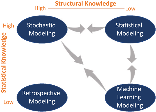
Generally speaking, the choice of modeling approaches and analytical techniques depends on our knowledge of the system under consideration. In the modeling language, the knowledge is translated into either statistical assumptions or structural assumptions of a model, which determine the domain of validation of the analysis. Conventionally, we may apply different approaches to model and analyze a system of interest, depending on the preciseness of the statistical and structural knowledge of the system; see Figure 1.

FIGURE 1

Conventional modeling approaches and the trends

When we are confident in the structural relationships between the inputs and outputs and in the statistical characterizations of uncertain factors, stochastic models are often developed to identify the decision that generates the optimal system performance. Most of the research in operations management falls into this category. For example, when applying the classical newsvendor model, we believe that the structure of the system is fully described by the facts that the amount of sales is the minimum of the demand and the order, that the price charged for all sold units is the same, and that the cost of all ordered units is the same. The statistical characterization (i.e., the distribution) of the uncertain demand is known. When we do not have much structural characterization of the system, we may impose statistical assumptions that we believe are appropriate, and adopt statistical models to analyze the system. For example, there may be multiple suppliers following different delivery processes, leading to a complex relationship between the procurement cost and the order quantity. In such a situation, we may apply an econometric model to understand the relationship between the earnings and the inventory levels by fitting some regression models that we believe are appropriate. Oftentimes, practitioners may have good structural knowledge (e.g., the amount of sales is limited by the inventory, or the procurement cost is linear), but may not have a good understanding of the statistical properties (e.g., the distribution family of the demand). In practice, retrospective models are often used to evaluate the decision performance and to identify improvement opportunities. When we do not have sufficient structural and statistical characterizations of the system, machine learning techniques are often applied.

There are certainly shades of gray, and Figure 1 does not specify all possible scenarios. For example, it is rare that we know nothing about the system. In reality, practitioners have their own experiences of how the system has worked and thus have some understanding of how the system may work in the future, though their knowledge may not be precise due to the changing environment. Thus, we make assumptions that are likely to reflect the reality, while enabling analytical tractability, and evaluate the robustness of the results obtained to understand the implication of the assumptions.

Arguably, complete structural and statistical characterizations of the system are unlikely to be obtained in reality. Data then become useful to understand the system and improve decision quality. The research trend we see recently is that a rapidly growing body of data‐integration work lies between the stochastic models and the statistical or machine learning models. And the emphasis has been given to relaxing the statistical assumptions and using data to supplement the knowledge gap. The approaches developed for specific problems are determined by both the domain of validation and the data generation model. The domain of validation is the collection of models, within which we believe the true model is. This domain is certainly determined by the structural and statistical assumptions of the true model. The data generation model determines the amount of information contained in the available data. For example, in a static or offline learning context, the data may be independent draws from some common distribution, and decisions are made after the realization of the random events associated with the data. In a dynamic or online learning context, the data may exhibit temporal dependence because of the learning strategy deployed. Moreover, observations may be censored by the chosen decisions, or feature variables may be useful to explain the observed variabilities.

Several articles, including Bastani et al. (2022b), Bertsimas and Kallus (2020), Mĭsić and Perakis (2020), Qi et al. (2020), and de Véricourt and Perakis (2020), have provided thorough surveys, insightful discussions, and visionary thoughts on data‐analytics research in operations management. It is certainly challenging to go beyond and unnecessary to repeat what has been discussed. Therefore, we attempt to focus on a niche by underscoring the aspect of data integration in operational decision‐making. We will describe a small subset of recent contributions in four major application areas to analyze what the common themes are, what the new philosophies are, where this research is heading, where the gaps are, and where POMS may provide leadership in the next decade.

DYNAMIC PRICING AND REVENUE MANAGEMENT

Arguably, the most researched application of data analytics in operations management is the design of pricing strategy; see Araman and Caldentey (2011) and den Boer (2015a) for excellent summaries. We choose to start our discussion from this application area because the key building block of modeling, the revenue function, has a simple structure (i.e., price multiplied by demand). The main ideas and intuitions behind the data‐integration approaches developed in this area can set the stage for understanding and comparing the developments in other application areas.

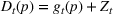
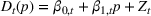
This line of studies focuses on situations with complete structural characterizations. Specifically, when a price p is charged, the subsequent demand is a random variable

D (p)

(with mean

λ (p)

), and the revenue is

p D (p)

. The goal is to find a sequence of prices that maximizes the total expected revenue over some planning horizon. Most studies assume that the demand can always be met, while some consider finite stock (e.g., Besbes & Zeevi, 2009; Cohen et al., 2018) and may include overage and underage costs into the objective function (e.g., Bertsimas & Perakis, 2006).

The statistical characterizations of the random demand

D (p)

are, however, incomplete. The commonly assumed demand models include Poisson demand (i.e.,

λ (p)

is the mean arrival rate), Bernoulli demand (i.e.,

λ (p)

is the purchase probability), or additive‐noise demand (i.e., the demand is

D (p) = λ (p) + Z

with Z being the random noise). The decision‐maker may lack knowledge of

λ (p)

, the noise distribution, or both. Instead, observations of

(p, D (p))

are used to determine the pricing strategy. When the additive‐noise model is adopted, it is typical to assume that the observed sample is generated with an independently and identically distributed (i.i.d.) or martingale‐difference sequence of errors.

Stationary price–demand relationship

When the demand is unknown, and data are progressively generated and observed, one may sequentially estimate the demand model using the available data and then optimize the price based on the estimated demand model. Such a solution, widely adopted in practice, is often termed the myopic policy in the literature. For example, Bertsimas and Perakis (2006) describe a stationary linear demand model with additive normal noise and unknown coefficients. They iteratively estimate the unknown coefficients using the observations so far, based on which the price is optimized. A myopic policy, while ensuring a high instantaneous profit (or revenue), can lead to incomplete learning (e.g., den Boer & Zwart, 2014; Rothschild, 1974). That is, there is a positive probability that the price path does not converge to the true optimal price. Moreover, depending on the pricing policy implemented, the estimated parameters may depend on the past price, which in turn depends on the demands observed up to then, creating price endogeneity.

To address the issue of incomplete learning, many authors have developed learning algorithms to obtain consistent solutions. We name a few examples. Harrison et al. (2012) demonstrate, using a Bernoulli demand, that incomplete learning can occur in the Bayesian dynamic programming model, which updates the distribution upon observing a demand and then optimizes the price based on the posterior distribution. They resolve the issue of incomplete learning by incorporating price experiments to create deviations from the myopic policy. Besbes and Zeevi (2009) consider a Poisson demand with an unknown random rate. Their algorithm divides the horizon into a learning phase and an earning phase. A sequence of pre‐selected prices is tested during the learning phase, at the end of which the mean demand rates are estimated using the sample averages. In the earning phase, the optimal price is selected based on the estimated demand rates. Besbes and Zeevi (2015) analyze an additive‐noise demand with unknown mean demand function and noise distribution. They divide the planning horizon into episodes, each containing a learning phase and an earning phase. During a learning phase, the myopic price and its perturbation are experimented. A linear demand is estimated using the least‐square estimation. The myopic price is then recomputed and implemented during the subsequent earning phase. Z. Wang et al. (2014) refine the algorithm by reducing the perturbation of the tested price over time. den Boer and Zwart (2014) consider a demand whose mean is a known increasing transformation of an unknown linear function (i.e.,

λ (p) = g (β_{0} + β_{1} p)

with g increasing and

β_{0}, β_{1}

unknown), and whose variance is an increasing function of the mean (i.e.,

Var [D (p)] = σ^{2} h (λ (p))

with

σ > 0

and h increasing). Thus, the maximum quasi‐likelihood estimate for

(β_{0}, β_{1})

can be computed. Whenever the sample variance of price is below a threshold, the price is optimized based on the estimates outside of the taboo interval, which contains the current sample average.

As a common theme, these studies attempt to combine the statistical estimation for the unknown demand function with the optimization of the pricing decision. This is done by balancing learning through exploring the suboptimal prices (i.e., price experiment) and earning through exploiting the revenue under the myopic price. The validation of the asymptotic efficiency under the designed policy (or, interchangeably, algorithm) is through regret minimization. That is, reducing the distance between the true optimal revenue and the revenue earned under the designed policy. The form of regret calculation depends on the price–demand relationship. With the Poisson demand, measuring the regret using the revenue ratio is appropriate as the mean rate equals the variance. With the additive‐noise demand, computing the regret as the revenue difference is natural, as the price only affects the mean of the demand distribution. To obtain a desirable regret bound, the algorithms proposed in the aforementioned studies attempt to achieve two conditions, in the language of Keskin and Zeevi (2015) (Theorem 2). First, the price experiments in the learning periods must create enough price dispersion. Second, the deviation of the implemented prices from the myopic price should be sufficiently infrequent. The first condition ensures that the estimation procedure discovers the true model quickly enough, and the second condition ensures that the revenue loss due to exploration reduces quickly enough.

The design of price experiments is essential to the performance of the learning algorithm. In reality, experiments do not come free. Cheung et al. (2017) impose a budget of price experiment (expressed as a maximum number m of price change) when the mean demand function comes from a known finite family. The algorithm divides the horizon into m episodes with the length iterated‐exponentially increasing. The first

(m - 1)

phases focus on learning the sample average, and the myopic optimal price is applied in the last phase to earn.

Incorporating demand features

When the demand exhibits dependence on some observable features (i.e., contextual information), the feature data can be used to improve the decision quality. For example, the search data from GoogleTrend may be used to understand the demand surge of certain consumer products. Consumers' browsing history on related webpages or consumers' past posts of product reviews may be related to their purchasing decisions. Such data can be incorporated into the demand model as a vector of observed feature variables (or covariates), denoted by x . The relation between the demand and the feature vector, often expressed through the feature coefficients in the demand model, can exhibit different patterns. An important consideration is the sparsity, reflected by the zero entries in the feature coefficients. For example, if the consumers are members of a store, then a complete record of some common features including gender, age, purchase frequency, and weekly spending may be maintained. In an online shopping environment, however, a store may have a record on distinct features for a small customer group, which are not relevant to other groups. It is typical in personalized marketing that the feature data are big but very sparse. The sparsity may make the relationship between the demand and the feature vector unidentifiable under conventional estimation techniques.

A commonly used measure for identifiability is the smallest eigenvalue of the empirical Fisher information matrix. When this eigenvalue is strictly positive, the matrix is invertible and thus the estimates can be computed. For example, Broder and Rusmevichientong (2012) consider a Bernoulli demand with the mean demand

λ (p, x)

in some parametric family. They assume that the smallest eigenvalue of the empirical Fisher matrix is above a constant defined by the parametric family. The algorithm explores the prices from a finite set during the learning phase and applies the myopic price based on the maximum‐likelihood estimates in the earning phase. Nambiar et al. (2019) consider a demand model

D (p) = β p + f (x) + Z

. Like Besbes and Zeevi (2009), they assume that the estimated

\hat{f}

is linear (with least‐square estimates identifiable from the data) but the true f is not. Due to the demand misspecification, the issue of price endogeneity arises, resulting in bias and inconsistency of the least square estimates. To counter this issue, they propose a random price shock algorithm. Specifically, the myopic price is perturbed by a Bernoulli distribution over

{- δ_{t}, δ_{t}}

with

δ_{t}

decreasing in time t. The random price shock acts like an instrumental variable, which depends on the price but is independent of the demand noise.

When the feature observations are sparse, price experiments, regularization terms, or clusters are often used to address the identifiability issue in estimation. Javanmard and Nazerzadeh (2019) analyze a Bernoulli demand with success probability

λ (p, x) = Pr {α \cdot x + Z > p}

, where α is the unknown parameter vector and Z has a known log‐concave distribution. They assume that the feature observations are generated independently from an unknown distribution with a positive definite variance–covariance matrix. Considering the high dimensionality of the estimation, they apply a regularized maximum likelihood which penalizes the likelihood function with the sum of absolute values of estimates. Ban and Keskin (2021) consider a demand model in which the feature vector and the price interacts (i.e.,

D (p) = (β \cdot x) p + α \cdot x + Z

with unknown

(α, β)

and distribution of Z). When the sparsity structure of the feature coefficients is known, the least square estimation can be obtained by ensuring that price dispersion over the learning periods increases at least in the order of

\sqrt{t}

. When the sparsity structure is unknown, the LASSO regularizer is included in the estimation, which penalizes nonzero coefficient estimates.

From a very different angle, Cohen et al. (2020) analyze the effect of demand feature by focusing on a special demand model, in which the customers' preference is deterministic but unknown. Specifically, a customer exhibiting feature x values the product at

α \cdot x

with α belonging to some uncertainty set. Given a sequence of distinct feature vectors

{x_{1}, x_{2}, …}

, the decision‐maker chooses a price for each feature vector. As the feature vectors are all distinct, the uncertainty set is shrinking in sequence, because a product is sold if and only if the price is below

α \cdot x

. The learning algorithm, instead of using statistical estimation, focuses on speeding up the bisectional search (through replacing the polytope of the uncertainty set by its ellipsoid).

Multiproduct and cross‐learning

The relationships among different products, though increasing the complexity of analysis, allow for leveraging the knowledge from one to understand the other. Cross‐learning happens when we have some partial characterization of the relationships among

{D_{i} (p), i \in M}

, where M is the set of products. Such relationships can be reflected through the commonality in feature relationships (e.g., common features), dependence in the joint distribution (e.g., correlated noise terms), or connection among marginal distributions (e.g., a common distribution family).

For example, Ferreira et al. (2016) consider multiple products and a finite set of feasible price vectors. The joint distribution of the product demands depends on the chosen price vector and some unknown parameters. The proposed algorithm adapts the Thompson sampling for parametric Bayesian learning (i.e., the multiarm bandit), which ensures price dispersion by probabilistically choosing suboptimal prices derived based on randomly sampled parameters from the posterior distribution. Bastani et al. (2022a) consider the multiproduct demand model

D_{i} (p_{i}) = (β_{i} \cdot x_{i}) p_{i} + α_{i} \cdot x_{i} + Z_{i}, i \in M

, that depends on product‐specific features x _i. The coefficients

((α_{i}, β_{i}), i \in M)

and the parameters of the jointly normal noise

(Z_{i}, i \in M)

are unknown. In the initial periods, prices are randomly selected until the variability of the posterior is sufficiently low, so that the smallest eigenvalue of the empirical Fisher matrix is sufficiently positive. The remaining horizon is divided into episodes with a fixed length, each for one product. In the earlier episodes, Thompson sampling is applied to the corresponding products. In the later episodes, the estimate of the posterior mean is computed as the average of least square estimates across all previous phases, facilitating transfer learning. These two papers, though applying different learning techniques, model the connection among the products through their statistical properties reflected by the joint demand distribution.

Connections among products can often be identified through cross price elasticities or through common features. Keskin et al. (2021b) analyze the demand model

D (p) = β_{0} + β_{1} \cdot p + Z

with β ₁ unknown. The price of one product may directly affect the demand of another. The coefficient matrix β ₁ exhibits certain known sparsity structures. They adopt a PAC (probably approximately correct)‐Bayesian approach that imposes a smooth regularizer on the estimation. The PAC‐Bayesian approach offers two advantages in situations with sparse features. First, it can significantly increase the computational efficiency. Second, the regularizer ensures that an unlikely observation does not significantly impact the posterior distribution, leading to robust estimates. Miao et al. (2022) consider a multiproduct model in which the arriving customer prefers a single product with a certain probability. Conditioning on the customer's preference

i \in M

, the demand follows a Bernoulli distribution with mean

λ_{i} (p_{i}, x_{i}) = g (α_{i} \cdot x_{i} + β_{i} p_{i})

, where

(α_{i}, β_{i})

are unknown and g is a known increasing function. The relation among the product demands is reflected by the similarity of the unknown coefficients. The proposed algorithm clusters products whose individual maximum‐likelihood estimates are close (within a threshold of the Euclidean distance). The maximum‐likelihood estimation is then applied to the product cluster to obtain the common coefficients.

Simchi‐Levi et al. (2021) discuss a problem with primary products and associated add‐on products, both having Bernoulli demands. In addition to selecting a price vector from a finite set, a discount may be offered to an add‐on product when the primary product is purchased. The proposed algorithm divides the horizon into episodes. In each episode, the upper‐confidence bounds on the average demands are constructed, based on which the prices within the episode are determined. To reduce performance loss, a terminal condition (i.e., enough observations for the selected add‐on product at the current price) is imposed which may end an episode before its planned length.

Many studies analyze multiproduct pricing decisions for choice‐based demands, we will postpone the discussion of these studies to Section 3, the section dedicated to choice‐based models.

Nonstationary environment

In reality, the demand distribution may change due to varying market conditions and customer tastes. The change may be reflected by different statistical properties, namely, demand variability (e.g., den Boer, 2015b), price sensitivity (e.g., Keskin & Zeevi, 2017), or feature‐based preference (e.g., Javanmard, 2017).

den Boer (2015b) studies the demand model

D_{t} (p) = g_{t} (p) + Z_{t}

with

g_{t}

known and the distribution of

Z_{t}

unknown. To account for the nonstationary demand process, they consider two modified least square estimates. Specifically, a moving window is imposed so that only observations within the last window are considered, or a polynomially decaying weight is applied based on how recent the observation is obtained. The nonstationarity is measured based on the weighted average of the squared deviation in the empirical demand noise, which depends on the choice of window size or decaying weight. They show that the myopic policy can produce a good performance with an appropriately chosen window size or decaying weight. Keskin and Zeevi (2017) consider a different demand model,

D_{t} (p) = β_{0, t} + β_{1, t} p + Z_{t}

, where the unknown coefficients

(β_{0, t}, β_{1, t})

may vary over time, while the random noise

Z_{t}

is i.i.d. The nonstationarity is measured by the maximum cumulative squared deviations of the unknown coefficients under any feasible pricing policy. They also consider learning with either a moving window or a decaying weight. An interesting finding from their analysis is that the performance increases when the change of coefficients takes place abruptly (vs. smoothly). Javanmard (2017) considers a feature‐dependent Bernoulli demand with mean

λ_{t} (p, x) = Pr {α_{t} \cdot x + Z_{t} \geq p}

, where

α_{t}

is unknown and time‐varying, while

Z_{t}

is i.i.d with known distribution. In each period, the unknown coefficients are estimated using projected gradient descent, and then the myopic price is computed based on the estimates and the observed features. The learning complexity depends on the time‐weighted cumulative variation in the coefficients.

In a different application, Zhang et al. (2022) study a Markovian Bass demand model. The proposed algorithm calls for setting a low price in the introductory stage when the initial data are collected. Then, iteratively, the parameters of the Bass model are estimated using the observed cumulative sales, based on which the price is optimized.

Remarks

The asymptotic performance of the policy has been the major focus of this research recently, which sets important theoretical foundations for understanding the associated dynamic pricing and revenue management problems. A regret bound of the order

\sqrt{T}

appears in many settings because the embedded statistical estimation approaches typically have an error bound of the order

\sqrt{T}

when the noise has a light tail (e.g., conditional sub‐exponential). The learning complexity depends critically on the statistical characterization of demand

D (p)

. It is important to appropriately choose the estimation technique that fits the application. For example, the regret bound may be improved to the order of

\log T

when the optimal revenue is higher than the revenue under any suboptimal price by a strictly positive constant. Such a situation arises when the revenue is strictly concave, and there are a finite number of feasible prices. In this case, learning can be sped up.

The presence of the uninformative price may increase learning complexity. For example, in the problem studied by Harrison et al. (2012), the uninformative price is the crossing point of the two possible mean demand curves. Incomplete learning may occur under the myopic price unless the uninformative price is not optimal for any Bayesian prior. Another example is discussed by Javanmard and Nazerzadeh (2019). The mean demand comes from a parametric family within which all demand curves intersect at a common price, and the common price is optimal for some feature values. A fast learning algorithm must produce significant deviations from the uninformative price, leading to a potential regret gap. A related concept is the discriminative price, at which all the mean demands are distinct. Knowledge of discriminative prices can reduce the learning complexity (see the related discussion in, e.g., Cheung et al., 2017).

We remark that our discussion in this section has omitted an important consideration, potentially limited inventories (e.g., Araman & Caldentey, 2011; Cheung et al., 2017). This consideration requires rather nonfundamental modifications of the learning process (e.g., including a shut‐off price at which the demand is zero almost surely), as the quantity is exogenously given. In Section 4, we will discuss the data‐integrated quantity decision and its critical differences from the price decision.

CHOICE, OPTIONS, AND PRICING

The axiom‐based mathematical modeling of choice dates back to the 1950s. Since then, the choice models have been extensively researched and continuously finding numerous applications in psychology, economics, marketing, and operations. With the wave of data analytics, many new contributions have been made recently in operations management.

Modeling, estimation, and identification

In general, a choice model describes how people would select a single element from a given set of options. Such a choice preference can be described by a probability vector

p (S) = (p_{i} (S), i \in S \cup {0})

, where S is the set of offered options and 0 stands for choosing nothing. Feng et al. (2022) summarize the existing choice models into four categories and show that each has an equivalent probability model representation.

The four categories of structural models are the attraction models, utility‐based models, temporal models, and rank‐list models, each describing the consumers' preference from a different angle. The attraction model assigns an attraction value to each option under the axiom of independence of irrelevant alternatives (Luce, 1959). These values represent the unnormalized choice probabilities. An attraction model is equivalent to a multinomial logit (MNL) model, though the latter is developed from the random utility model. A random utility model assigns a random consumption utility to each option. A consumer's utility vector is an independent random realization, and the consumer chooses the maximum‐utility option within the available set. Extensions of MNL (e.g., nested logit, mixed logit, and latent MNL) models, probit models, and exponomial models belong to this category. A temporal model assumes that the consumer's preference is described by the occurrence of some random events, one related to an option. The consumer would choose the option corresponding to the earliest event among the available options. The Markov‐chain choice model developed by Blanchet et al. (2016) and Gupta and Hsu (2020), the single‐transition model by Nip et al. (2021), and the k‐attempt model by Chung et al. (2019) are examples of temporal models. Under a rank‐list model, each consumer has a rank order of all the options and would choose the highest ranked option from the available ones. A consumer's type is a random draw from a discrete random variable (index), which determines the rank list of that consumer. It turns out that the last three categories of models coincide—A model in one category has an equivalent representation in each of the other two categories (Feng et al., 2022). Thus, the estimation method developed for one can be applied to others.

The estimation and identification of a structural choice model with data are nontrivial as the number of potential offering sets can be large. Even in the parametric setting, the likelihood function may not be well behaved and a considerable effort is made to develop efficient estimation approaches like expectation maximization (e.g., Train, 2008; van Ryzin & Vulcano, 2017).

A major focus in recent research is to identify the right choice model using data with relaxed structures (e.g., partially nonparametric) or additional structures. A relaxation can significantly increase the complexity in model estimation, requiring the development of optimization techniques. For example, Ho‐Nguyen and Kılınç‐Karzan (2021) formulate a min‐max (saddle point) model to estimate the rank‐list distribution and analyze the sparsity of the estimates. Farias et al. (2013) use a pairwise preference matrix to represent rank lists, which account for the censored observations of the full rank list. Based on this representation, the potential models that can generate the observed data are characterized through linear constraints, and then the pessimistic (worst‐case) revenue is estimated. van Ryzin and Vulcano (2015) analyze a similar problem and apply column generation to reduce the computational burden in estimation. Specifically, the maximum‐likelihood estimates are computed over a subset of rank lists. Then the algorithm explores additional rank lists to improve the estimates. Chen and Mišić (2022) relax the rationality assumption of many random utility models by allowing the choice probability to increase when additional options are added to the offered set. A customer's type is described as a binary‐choice tree. The consumer starts from the root of the tree, moves down to the left or right child depending on whether the option associated with the current node is offered, and chooses the option associated with the leaf node. This paper discusses the complexity of model identification and proposes techniques (column generation and randomized tree sampling) for estimation.

Several studies analyze elaborated consumer behaviors that are not captured in conventional models. Jagabathula and Vulcano (2018) refine the choice model using the fact that the consumer may have a random consideration set. Options outside of the consideration set, even offered, would not be chosen. They use a set of acyclic directed trees to identify consumers' partial preferences based on data, and analyze an integer program to obtain the estimates. Jagabathula et al. (2021) consider a general model of the consumer's consideration set. They develop an approach to solve the mixed‐integer nonlinear optimization problem for the maximum‐likelihood estimation. The model proposed by Ferreira et al. (2022) (see Section 3.2) is another representative example.

Feng et al. (2022) apply a framework, called operational data analytics, developed by Feng and Shanthikumar (2022), to bridge the gap between parametric and nonparametric estimations. This approach takes into account possibly imprecise (“roughly correct”) structural assumptions in validating the estimated model. A class of estimation functions (i.e., operational statistics) is developed to leverage the structure implied by the domain knowledge and the information contained in the observed data. The optimal estimation function is derived by validating the regret of the estimation error over a set of models that may or may not satisfy the structural assumptions. This approach not only produces an estimate of the choice model but also identifies the true structure if the underlying model comes from a collection of structural models.

All these studies perform static learning of the choice model by assuming that the data generation is independent of the estimation approach adopted. An important aspect of model identification, currently underresearched, is how to design the experiment (by selecting a sequence of offered sets) so that the “most useful” data are generated under a limited learning budget. It is worth mentioning that Fisher et al. (2018) conduct a field experiment and make several interesting observations empirically, though their focus is not to provide guidance for experimental design.

Choice‐based product assortment, display, and pricing

The consumer choice model has been the building block for price and revenue optimization (Strauss et al., 2018) and assortment planning (Chernev, 2011; Karampatsa et al., 2017).

A natural way of data‐integrated decision‐making is the learning‐then‐earning approach, with which the choice model is estimated from historical data and the decisions are then optimized based on the estimated model. Yan et al. (2022) design price experiments to estimate the random utility model and develop algorithms to optimize the product prices. Jena et al. (2020) consider assortment planning under partially ranked consumer preference in the spirit of Farias et al. (2013), which allows the consumer to be indifferent among a subset of options. Using a column‐generation approach similar to that developed by van Ryzin and Vulcano (2015), they solve for the optimal assortment decision from an integer program. Jagabathula and Rusmevichientong (2017) analyze the optimization of assortment and prices when consumers' choices are limited to their own consideration sets. They develop an expectation maximization approach to obtain the maximum‐likelihood estimate of the choice model and design an algorithm to compute profit‐maximizing decisions. Paul et al. (2018) use a tree representation of consumer choice. Based on historical sales data, a greedy heuristic is deployed to identify possible rank lists that could have possibly generated the data. The fitted trees and consumer type distribution (over all possible rank lists) are estimated using maximum likelihood. Then, the dynamic assortment and pricing decisions are optimized.

Different approaches for dynamic learning and earning have been explored by several authors. Bernstein et al. (2019) apply a dynamic Bayesian framework with a Dirichlet prior on the consumer's preference. The planning horizon is divided into episodes with equal length. In each episode, the clusters of consumer types are updated based on the observations from the last episode. The estimated choice probabilities are updated, and a multiarm bandit algorithm is deployed to select the assortment. Chen et al. (2022a) consider feature‐based dynamic pricing under an MNL choice model. They use a constrained maximum‐likelihood estimation to account for the potential sparsity of the coefficients. Chen et al. (2020b) examine dynamic assortment decisions in a similar setting. During the initial learning phase, the assortment is chosen by uniformly sampling all possible offerings. Then the maximum‐likelihood estimators are computed for the choice model. In the remaining periods, the estimated choice model is updated based on the observed features and revenues using a constrained maximum‐likelihood estimation and the upper‐confidence bounds are constructed to determine the assortment.

Consumer choice models have been applied to analyze offering decisions in related, but different contexts. For example, Ferreira et al. (2022) model the consumer's choice of clicking on products. The choice probability can be shifted (by an additive term) based on the products clicked before. Each consumer is associated with a display window beyond which the consumer would not browse. The focus is to design a display sequence (a ranked list) that maximizes the number of consumers who click on at least one product. The proposed algorithm iteratively adds a product to the current list, experiments with the display to obtain response data, and then decides, based on a threshold response rate, whether or not to keep the newly added product on the list. In a related context, Gao et al. (2022) consider a cascade‐click model for the consumer purchase choice. They develop contextual‐based (i.e., click‐based) upper confidence bounds for dynamic learning and price optimization.

Remarks

Structural models that exhibit nice properties may not fit data, while fully nonparametric models are complex to identify (Chen et al. 2021c). In particular, the number of parameters needed to be estimated for a full rank‐list model is

m! \times m

, where m is the number of products. The complexity of model estimation and decision optimization can be reduced by focusing on a limited number of rank lists (van Ryzin & Vulcano, 2015) or on partial rankings (Bernstein et al., 2019; Jagabathula et al., 2021; Jena et al., 2020). Allowing unranked options or assuming consideration sets is essentially equivalent to clustering the consumer types (reflected by the rank lists).

Implementing choice‐based models and solutions in practice requires a careful treatment of many details. An insightful discussion can be found in Vulcano et al. (2017), which demonstrates empirical considerations in the choice‐model design for revenue maximization.

PROCUREMENT, INVENTORY, AND PRICING

Managing material flows to meet the uncertain demands has been the forever puzzle faced by practitioners. Many approaches for data‐based decision‐making have been developed in the operations management research.

Offline‐learning newsvendor

The newsvendor model is probably the most studied model in the operations management literature. It is probably the one with the earliest development in data‐integrated decision‐making that departs from the paradigms of learning‐then‐earning (i.e., predetermined learning phase and earning phase) and learning‐or‐earning (i.e., probabilistically determined learning or earning period by applying, e.g., Thompson sampling or upper‐confidence bounds). This departure leads to a direct data‐integration approach that does not separate learning (i.e., parameter estimation) and earning (i.e., decision optimization).

Hayes (1969) first describes a data‐integrated newsvendor solution by defining the mismatch cost as the loss function and the ordering decision as a statistics. Pointing out the asymmetry of the loss function, he argues that the data‐integrated solution is naturally biased. This observation is further elaborated by Siegel and Wagner (2021) in their analysis of exponentially distributed demands. Several authors (Akcay et al., 2011; Janssen et al., 2009) have proposed solutions to adjust the safety stock factor derived from the estimated demand, leveraging both the sample information and the profit optimization. A general data‐integrated solution is developed by Chu et al. (2008), who define the decision as a direct function of data using the concept of operational statistics proposed by Liyanage and Shanthikumar (2005). This approach produces a uniformly optimal ordering decision as a statistics of the demand data.

All the above studies assume a known distribution family of the demand. When there is no knowledge about the demand distribution (i.e., in nonparametric settings), the estimation of the distribution parameters needs to be expanded to that of the distribution function, as the optimization of the newsvendor model requires the input of demand distribution. One learning‐then‐earning approach here is to apply quantile regression (see, e.g., Amrani & Khmelnitsky, 2017; Harsha et al., 2021) and optimize the decision based on the quantiles.

To break the separation between learning and earning in a nonparametric setting, a natural approach is to examine the average profit computed by replacing the random demand with the demand samples. This is the sample‐average approximation (SAA), which, under the standard structural assumptions of the newsvendor model, is equivalent to the retrospective analysis and the approximation using empirical distribution. Certainly, a pure SAA would result in overfitting. The common approach is to either add a regularizer to the estimated profit or impose a constraint to control the variability of the estimated profit (see, e.g., Cheung & Simchi‐Levi, 2019; Homem‐de‐Mello & Bayraksan, 2014; Levi et al., 2007, 2015; Qin et al., 2022).

Recognizing that the (unregularized) SAA solution corresponds to a specific order statistics of the demand data, Besbes and Mouchtaki (2021) focus on a class of operational statistics that are mixtures of order statistics. They demonstrate the superiority of the resulting solution against the existing ones in the small‐sample regime. Taking a different angle, Lin et al. (2021) modify the empirical profit, instead of the empirical solution, by computing a weighted retrospective profit. The weights are estimated using clustering techniques (i.e., the k‐nearest neighborhood, kernel regression, or classification and regression tree). Ban and Rudin (2019) incorporate demand features into the analysis and apply Kernel regression to estimate the mean demand.

Research considering the endogenous pricing decision often assumes a demand model with an additive noise, that is,

D (p) = λ (p) + Z

(or, sometimes, a multiplicative noise, i.e.,

D (p) = Z λ (p)

). Many estimation approaches used in dynamic pricing and revenue management problems discussed in Section 2 have been applied to learn the mean demand function (e.g., Qin et al., 2022), while the distribution of Z, in the nonparametric setting, is often estimated using the empirical distribution or quantiles (e.g., Harsha et al., 2021). For parametric demand models, Chu et al. (2022) develop an operational data analytics framework that consists of a data‐integration model and a validation model. They show that the operational statistics of the ordering decision derived from this framework are uniformly optimal. This framework also generates an estimated profit function, from which the optimized price reveals significantly superior performance against that under the learning‐then‐earning approach especially when the sample size is small.

An alternative approach for data integration is robust optimization (Bertsimas & Thiele, 2006; Bertsimas & Vayanos, 2017; Lu & Shen, 2021). For example, Hu et al. (2019) define a candidate set of mean demand functions by bounding the squared deviation when fitted from the observed data. The mean demand is used to replace the random demand in approximating the profit function, based on which the worst candidate demand function is chosen under the optimal pricing and inventory policy.

Dynamic learning

When considering dynamic learning, many studies also relax the structural assumptions of the newsvendor model by allowing (partial) inventory carryover, positive delivery lead times, or fixed ordering costs. Most of the learning algorithms use episodic update and re‐optimization, like those in the pricing and revenue management literature, and focus on balancing the estimation error, approximation error, and profit generation.

For the classical period‐review inventory problem, Chen et al. (2019) design an algorithm similar to that of Besbes and Zeevi (2015) by experimenting on two prices and their corresponding order‐up‐to levels during the learning phase. They use a linear approximation to estimate the mean demand and compute the noise. A potential challenge in data‐integrated inventory planning is the possibility of censored demand observations. Indeed, Ban (2020) suggests that the bias‐corrected demand estimates from the censored observations may lead to inconsistent inventory decisions. She adjusts the profit estimation using the censored observations instead. Zhang et al. (2020) propose that, in parallel to the actual system, a shadow system is simulated with a base‐stock level lower than its counterpart in the actual system. The shadow system only runs in periods when the inventory is sufficient to meet the demand. The parallel system allows for best utilizing the observed data and facilitating the evaluation of the cost gradient, which is used to update the base‐stock level to be implemented in the next episode. To address the issue of demand censoring in making price and inventory decisions, Chen et al. (2021a) use a spline approximation for the unknown mean demand function with spline coefficients computed from the data in the learning phase.

When fixed ordering costs are paid, Yuan et al. (2021) propose an algorithm to find the optimal

(s, S)

policy. Each episode starts by setting the highest order‐up‐to level and the lowest reorder point among a candidate set. Such a choice allows for computing the costs for all candidate policies after observing the sales within the episode, and thus the stochastic gradient can be computed to narrow down the region for policy search based on a confidence bound. Chen et al. (2021b) further consider the endogenous price decision in this problem. They design upper‐confidence bounds for price learning and construct quantile estimations for the demand noise.

Considering nonstationary demands, Keskin et al. (2022a) model time‐varying demand coefficients and i.i.d. additive noise. Their algorithm divides the horizon into episodes of equal length, each consisting of a learning phase and an earning phase. To account for the nonstationarity in the demand, change detection is performed on the deviation among average demands after conducting price experiments in each learning phase to determine whether historical data should be discarded. Keskin et al. (2021) study a similar problem in a nonparametric setting. They deploy a time‐window policy, in a spirit similar to that used by den Boer (2015b) and Keskin and Zeevi (2017) and discuss the difference in the learning complexity between the pricing decision and the ordering decision. Chen (2021) considers inventory control under unknown discrete demand distributions and derives performance bounds for exploration‐heavy or exploitation‐heavy learning algorithms.

Remarks

Learning of pricing decisions and inventory decisions can be very different when we compare the developments discussed in this section with those in Section 2. For a pure pricing policy, the focus is to discover the mean demand curve. Many statistical methods (e.g., least square, maximum likelihood) used for learning the mean demand curve may not be sufficient to make an inventory decision. Instead, estimation of the distribution function (e.g., empirical distribution, quantile, order statistics) is needed.

We also note that there are studies of more sophisticated structural models, including capacitated production (Chen et al. 2020a) and dual sourcing (Chen & Shi, 2021).

HEALTHCARE OPERATIONS

Healthcare is gaining significant attention in many fields. Research in our field centers around issues associated with understanding, predicting, and optimizing the performance of resource planning (e.g., staffing, bed occupancy, drug approval), resource allocation (e.g., admission, diversion, discharging, organ matching, scheduling), and quality management (e.g., treatment outcome, test accuracy, readmission, drug safety). The applications are diverse, and each brings unique considerations in modeling and analysis. These are evident from recent surveys by several experts in our field (Anderson et al., 2022; Baron, 2021; Betcheva et al., 2020; Diwas Singh et al., 2020; Hopp et al., 2018; Keskinocak & Savva, 2020).

The current status and recent trends

The studies on healthcare operations are heavily centered on the two corners in Figure 1, namely, statistical modeling and stochastic modeling. For the former, empirical approaches (e.g., econometric models, hypothesis testing) are applied to analyze real data (recent examples include Bobroske et al., 2022; Lan et al., 2022; Niewoehner & Staats, 2022). In these studies, the input–output relationship is often modeled at a high level with time aggregation, without the detailed structures to enable decision optimization. In the second stream of healthcare research, analytical models are formulated and techniques including stochastic program, approximate dynamic program, Bayesian dynamic program, queuing analysis, and equilibrium analysis are used to derive the decisions (recent examples include Adida, 2021; Ahuja et al., 2021; Ata et al., 2020; Bavafa et al., 2022; Carew et al., 2021; Slaugh et al., 2018; Tian et al., 2022). In these studies, data are often not explicitly modeled as an input to the decision models, though some demonstrate how to apply the model to real data (e.g., Aswani et al., 2019).

Both research streams, though appearing separately from each other, exhibit a trend of adopting machine learning techniques. To draw inferences from empirical studies, machine learning techniques are used to replace traditional econometrics methods to relax relational assumptions or to deal with high dimensionality. For example, Schiele et al. (2021) use features extracted from data to formulate an estimation model using a neural network and apply gradient descent to obtain estimates for bed occupancy. Wang et al. (2022) adopt casual trees with instrumental variables to identify heterogeneous treatment effects. Xu et al. (2021) apply text mining to understand how online reviews impact the patient choice of care providers.

In stochastic modeling, a recent focus is on combining machine learning methods with conventional approaches to facilitate data integration and address the computational complexity. For example, Shi et al. (2021) use clustering, expectation maximization, and instrumental variables to estimate patient readmission time based on patient features. The estimates are used as inputs to an approximated Markov decision process from which the patient discharging policy is optimized. Grand‐Clément et al. (2021) examine a Markov decision process for cost‐efficient resource allocation based on patients' health states. They use classification trees to identify an allocation policy and demonstrate the application of the approach using the retrospective data of COVID‐19 hospitalization cases. Bravo et al. (2022) propose a queuing network framework to model clinical trials for new drugs and estimate the model parameters from data to demonstrate the implementation of the drug‐specific approval policy. Xie et al. (2022) examine patient overflow by defining a bed shortage measure using a notion similar to the quasi‐convex risk measure. This measure can be computed using the patient flow data. Based on this measure, they formulate an optimization model to plan bed capacity.

The majority of these studies belong to the static learning‐then‐earning paradigm, applying statistical machine learning techniques on data to obtain inputs for decision‐making. There are a few recent studies deviating from this paradigm. For example, Bastani and Bayati (2021) develop a LASSO bandit algorithm for problems involving high‐dimensional features and derive the bounds of the expected regret. They demonstrate the application of the algorithm to determine the warfarin dosage based on patients' features. Bastani et al. (2021) use LASSO and empirical Bayes to identify key features for travelers' type and apply reinforcement learning to evaluate COVID‐19 testing policies. Anderer et al. (2022) study clinical trial design. They apply a proportional hazard rate model for the trial outcome and use a Bayesian framework to estimate the effect based on patient‐level data. The patient enrollment level and the target posterior variance are chosen to minimize the expected cost under given type I and type II error requirements. Chan et al. (2022) model patients' journeys in the healthcare system by capturing possible deviations from the reference pathways. Using the data of patients' medical records, they apply inverse optimization to identify the patients' cost structures in the network.

Potential directions and challenges

Though the research on healthcare operations spans over a wide range of topics, the conventional views are often hospital focused (i.e., appointment and resource scheduling, resource planning, and allocation), disease focused (admission, matching, treatment), or medicine focused (development, approval, production, insurance, financing). As detailed patient data become available, there is a movement toward patient‐centric approaches (in, e.g., therapeutic development, information display, self‐management intervention); see the POM special issue edited by Bretthauer and Savin (2018). Such a movement calls for personalized predictive and prescriptive models to improve the precision of medical decision‐making. Though machine learning is finding increasing applications in healthcare, most of the publications appear in medical and computer science journals with an emphasis on performance assessment and predictability. From the operations perspective, there is plenty of room for data‐integrated medical decision‐making and experimental design in various applications.

The research in healthcare, compared with that in other areas, has its unique challenges. Different healthcare providers may maintain different practices, procedures, and protocols. Data sharing across providers remains a difficult task in many situations. Moreover, a solution approach developed for one may not be directly applicable to another, and the results obtained from one application may not be replicable in another, even very similar, application. Anderson et al. (2022) summarize five main barriers to realizing the practical values of research findings, including the resistance from practitioners, the competition among providers, the quality of data, the mismatch of incentive, and the nontransferability of solutions. Fundamental work on general frameworks that address these challenges is yet to be developed.

DISCUSSION AND FURTHER DIRECTIONS

Data analytics is finding increasing applications and making a major shift in the research of operations management. With the consideration of data, researchers are not only developing new models and new approaches for traditional operations problems, but also discovering new problems and issues, for example, privacy‐proof policies (Chen et al. 2022b), personalized bundle pricing (Ettl et al., 2020), reusable resources (Gong et al., 2022), crowd sourcing (Manshadi & Rodilitz, 2022), personalized priority (Hathaway et al., 2022), and racial bias (Samorani et al., 2021). As we have seen from our discussions, there are many ways of data integration, and the choice of the approach must match with the application and the goal of the analysis.

To push the frontier of data analytics in operations management, an increasing amount of theoretical research is the engine. Many scholars have made important theoretical contributions under general frameworks (e.g., Aswani et al., 2018; Besbes et al., 2014; Elmachtoub & Grigas, 2022; Gupta & Kallus, 2022; Gupta & Rusmevichientong, 2020; Zhu et al. 2022). These developments have great potential to generate new understandings in different application domains. The development of new paradigms that blur the boundaries between the conventional modeling approaches would lead to breakthroughs of the research on many operations problems. Moreover, relaxing the technical conditions that are commonly assumed in our analytical and empirical models (e.g., linearity, concavity, log‐linearity, additivity) can enhance the data integration into decision models. For example, many studies assume that the revenue function is smooth and concave in price. Though necessary for analytical elegance, such a condition may not be satisfied and may be difficult to verify in reality. Improving the resilience of the learning approach along this dimension (e.g., Wang et al., 2021) is valuable to practice.

Admittedly, the gap between the research and application exists. Execution of many proposed policies can be challenging in practice unless one has extensive knowledge of the theories. Simple algorithms and easy‐to‐follow implementation procedures can make the research development accessible to the practitioners. For example, in dynamic pricing, the price dispersion needs to be of order

\sqrt{t}

to ensure the desired speed of learning. Is there a simple rule to choose the multiplier of

\sqrt{t}

based on the operating parameters? Developing solutions with implementation awareness can significantly increase the value of research contributions.

Footnotes

ACKNOWLEDGMENTS

The authors are grateful to Christopher Tang for his helpful suggestions.

References

Adida

(2021). Outcome‐based pricing for new pharmaceuticals via rebates. Management Science, 67(2), 892–913.

Ahuja

Alvarez

C. A.

Birge

J. R.

Syverson

(2021). Enhancing regulatory decision making for postmarket drug safety. Management Science, 67(12), 7493–7510.

Akcay

Biller

Tayur

(2011). Improved inventory targets in the presence of limited historical demand data. Manufacturing & Service Operations Management, 13(3), 297–309.

Amrani

Khmelnitsky

(2017). Estimation of quantiles of non‐stationary demand distributions. IISE Transactions, 49(4), 381–394.

Anderer

Bastani

Silberholz

(2022). Adaptive clinical trial designs with surrogates: When should we bother? Management Science, 68(3), 1982–2002.

Anderson

Bjarnadottir

M. V.

Nenova

(2022). Machine learning in healthcare: Operational and financial impact. In Babich

Birge

J. R.

Hilary

(Eds.) Innovative technology at the interface of finance and operations (pp. 153–174). Springer Series in Supply Chain Management, Vol. 11. Springer, Cham.

Araman

V. F.

Caldentey

(2011). Revenue management with incomplete demand information. In Wiley Encyclopedia of Operations Research and Management Science (pp. 1–17). John Wiley & Sons.

Aswani

Shen

Z.‐J. M.

Siddiq

(2018). Inverse optimization with noisy data. Operations Research, 66(3), 870–892.

Aswani

Shen

Z.‐J. M.

Siddiq

(2019). Data‐driven incentive design in the medicare shared savings program. Operations Research, 67(4), 1002–1026.

10.

Ata

Ding

Zenios

(2020). An achievable‐region‐based approach for kidney allocation policy design with endogenous patient choice. Manufacturing & Service Operations Management, 23(1), 580–599.

11.

Ban

G.‐Y.

(2020). Confidence intervals for data‐driven inventory policies with demand censoring. Operations Research, 68(2), 309–326.

12.

Ban

G.‐Y.

Keskin

N. B.

(2021). Personalized dynamic pricing with machine learning: High dimensional features and heterogeneous elasticity. Management Science, 67(9), 5549–5568.

13.

Ban

G.‐Y.

Rudin

(2019). The big data newsvendor: Practical insights from machine learning. Operations Research, 67(1), 90–108.

14.

Baron

(2021). Business analytics in service operations—Lessons from healthcare operations. Naval Research Logistics, 68, 571–533.

15.

Bastani

Bayati

(2021). Online decision making with high‐dimensional covariates. Operations Research, 68(1), 276–294.

16.

Bastani

Drakopoulos

Gupta

Vlachogiannis

Hadjicristodoulou

Lagiou

Magiorkinis

Paraskevis

Tsiodras

(2021). Efficient and targeted COVID‐19 border testing via reinforcement learning. Nature, 559, 108–113.

17.

Bastani

Simchi‐Levi

Zhu

(2022a). Meta dynamic pricing: Transfer learning across experiments. Management Science, 68(3), 1865–1881.

18.

Bastani

Zhang

D. J.

Zhang

(2022b). Applied machine learning in operations management. In Babich

Birge

J. R.

Hilary

(Eds.) Innovative Technology at the interface of finance and operations (pp. 189–222). Springer Series in Supply Chain Management, Vol. 11. Springer, Cham.

19.

Bavafa

Örmeci

Savin

Virudachalam

(2022). Surgical case‐mix and discharge decisions: Does within‐hospital coordination matter? Operations Research, 70(2), 990–1007.

20.

Bernstein

Modaresi

Sauré

(2019). A dynamic clustering approach to data‐driven assortment personalization. Management Science, 65(5), 2095–2115.

21.

Bertsimas

Kallus

(2020). From predictive to prescriptive analytics. Management Science, 66(3), 1025–1044.

22.

Bertsimas

Perakis

(2006). Dynamic pricing: A learning approach. In Lawphongpanich

Hearn

D. W.

Smith

M. J.

(Eds.), Mathematical and computational models for congestion charging (pp. 45–79). Springer.

23.

Bertsimas

Thiele

(2006). A robust optimization approach to inventory theory. Operations Research, 54(1), 150–168.

24.

Bertsimas

Vayanos

(2017). Data‐driven learning in dynamic pricing using adaptive optimization. Optimization Online . https://optimization‐online.org/2014/10/4595/

25.

Besbes

Gur

Zeevi

(2014). Stochastic multi‐armed‐bandit problem with non‐stationary rewards. In Ghahramani

Welling

Cortes

Lawrence

Weinberger

K.Q.

(Eds.), Advances in Neural Information Processing Systems 27 (NIPS 2014) (pp. 199–207). MIT Press.

26.

Besbes

Mouchtaki

(2021). How big should your data really be? Data‐driven newsvendor and the transient of learning (Working paper), Columbia University, New York, NY. Available at: https://ssrn.com/abstract=3878155

27.

Besbes

Zeevi

(2009). Dynamic pricing without knowing the demand function: Risk bounds and nearoptimal algorithms. Operations Research, 57(6), 1407–1420.

28.

Besbes

Zeevi

(2015). On the (surprising) sufficiency of linear models for dynamic pricing with demand learning. Management Science, 61(4), 723–739.

29.

Betcheva

Erhun

Jiang

(2020). OM Forum—Supply chain thinking in healthcare: Lessons and outlooks. Manufacturing & Service Operations Management, 23(6), 1333–1353.

30.

Blanchet

Gallego

Goyal

(2016). A Markov chain approximation to choice modeling. Operations Research, 64(4), 886–905.

31.

Bobroske

Freeman

Huan

Cattrell

Scholtes

(2022). Curbing the opioid epidemic at its root: The effect of provider discordance after opioid initiation. Management Science, 68(3), 2003–2015.

32.

Bravo

Corcoran

T. C.

Long

E. F.

(2022). Flexible drug approval policies. Manufacturing & Service Operations Management, 24(1), 542–560.

33.

Bretthauer

K. M.

Savin

(2018). Introduction to the special issue on patient‐centric healthcare management in the age of analytics. Production and Operations Management, 27(2), 2101–2102.

34.

Broder

Rusmevichientong

(2012). Dynamic pricing under a general parametric choice model. Operations Research, 60(4), 965–980.

35.

Carew

Nagarajan

Shechter

Arneja

Skarsgard

(2021). Dynamic capacity allocation for elective surgeries: Reducing urgency‐weighted wait times. Manufacturing & Service Operations Management, 23(2), 407–424.

36.

Chan

T. C. Y.

Eberg

Forster

Holloway

Ieraci

Shalaby

Yousefi

(2022). An inverse optimization approach to measuring clinical pathway concordance. Management Science, 68(3), 1882–1903.

37.

Chen

(2021). Data‐driven inventory control with shifting demand. Production and Operations Management, 30(5), 1365–1385.

38.

Chen

Chao

Ahn

H.‐S.

(2019). Coordinating pricing and inventory replenishment with nonparametric demand learning. Operations Research, 67(4), 1035–1052.

39.

Chen

Chao

Shi

(2021a). Nonparametric learning algorithms for joint pricing and inventory control with lost sales and censored demand. Mathematics of Operations Research, 46(2), 726–756.

40.

Chen

Simchi‐Levi

Wang

Zhou

(2021b). Dynamic pricing and inventory control with fixed ordering cost and incomplete demand information. Management Science, 68(8), 5684–5703.

41.

Chen

Gallego

Tang

(2021c). Estimating discrete choice models with random forests. In Qiu

Lyons

Chen

(Eds.) AI and analytics for smart cities and service systems (ICSS 2021) (pp. 184–196). Lecture Notes in Operations Research. Springer, Cham.

42.

Chen

Shi

Duenyas

(2020a). Optimal learning algorithms for stochastic inventory systems with random capacities. Production and Operations Management, 29(7), 1624–1649.

43.

Chen

Shi

(2021). Tailored base‐surge policies in dual‐sourcing inventory systems with demand learning (Working paper). University of Illinois at Chicago, Chicago, IL. Available at: https://ssrn.com/abstract=3456834

44.

Chen

Owen

Pixton

Simchi‐Levi

(2022a). A statistical learning approach to personalization in revenue management. Management Science, 68(3), 1923–1937.

45.

Chen

Simchi‐Levi

Wang

(2022b). Privacy‐preserving dynamic personalized pricing with demand learning. Management Science, 68(7), 4878–4898.

46.

Chen

Wang

Zhou

(2020b). Dynamic assortment optimization with changing contextual information. Journal of Machine Learning Research, 21, 1–44.

47.

Chen

Y.‐C.

Mišić

V. V.

(2022). Decision forest: A nonparametric approach to modeling irrational choice. Management Science. Advance online publication. https://doi.org/10.1287/mnsc.2021.4256

48.

Chernev

(2011). Product assortment and consumer choice: An interdisciplinary review. Foundations and Trends in Marketing, 6(1), 1–61.

49.

Cheung

W. C.

Simchi‐Levi

(2019). Sampling‐based approximation schemes for capacitated stochastic inventory control models. Mathematics of Operations Research, 44(2), 668–692.

50.

Cheung

W. C.

Simchi‐Levi

Wang

(2017). Dynamic pricing and demand learning with limited price experimentation. Operations Research, 65(6), 1722–1731.

51.

Chu

Feng

Shanthikumar

J. G.

Shen

Z.‐J. M.

(2022). Solving the price‐setting newsvendor problem with parametric operational data analytics (ODA) (Working paper). Purdue University, West Lafayette, IN.

52.

Chu

L. Y.

Shanthikumar

J. G.

Shen

Z. J. M.

(2008). Solving operational statistics via a Bayesian analysis. Operations Research Letters, 36, 110–116.

53.

Chung

Ahn

H.‐S.

Jasin

(2019). (Rescaled) multi‐attempt approximation of choice model and its application to assortment optimization. Production and Operations Management, 28(2), 341–353.

54.

Cohen

M. C.

Lobel

Leme

R. P.

(2020). Feature‐based dynamic pricing. Management Science, 66(11), 4921–4943.

55.

Cohen

M. C.

Lobel

Perakis

(2018). Dynamic pricing through data sampling. Production and Operations Management, 27(6), 1074–1088.

56.

deVéricourt

Perakis

(2020). Frontiers in service science: The management of data analytics services: New challenges and future directions. Service Science, 12(4), 121–129.

57.

den Boer

A. V.

(2015a). Dynamic pricing and learning: Historical origins, current research, and new directions. Surveys in Operations Research and Management Science, 20(1), 1–18.

58.

den Boer

A. V.

(2015b). Tracking the market: Dynamic pricing and learning in a changing environment. European Journal of Operational Research, 247(3), 914–927.

59.

den Boer

A. V.

Zwart

(2014). Simultaneously learning and optimizing using controlled variance pricing. Management Science, 63(4), 965–978.

60.

Diwas Singh

K. S.

Scholtes

Terwiesch

(2020). Empirical research in healthcare operations: Past research, present understanding, and future opportunities. Manufacturing & Service Operations Management, 22(1), 73–83.

61.

Elmachtoub

A. N.

Grigas

(2022). Smart “predict, then optimize.” Management Science, 68(1), 9–26.

62.

Ettl

Harsha

Papush

Perakis

(2020). A data‐driven approach to personalized bundle pricing and recommendation. Manufacturing & Service Operations Management, 22(3), 461–480.

63.

Farias

Jagabathula

Shah

(2013). A nonparametric approach to modeling choice with limited data. Management Science, 59(2), 305–322.

64.

Feng

Shanthikumar

J. G.

(2022). The framework of parametric and non‐parametric operational data analytics (ODA) (Working paper). Purdue University, West Lafayette, IN.

65.

Feng

Shanthikumar

J. G.

Xue

(2022). Consumer choice models and estimation: A review and extension. Production and Operations Management, 31(2), 847–867.

66.

Ferreira

K. J.

Lee

B. H. A.

Simchi‐Levi

(2016). Analytics for an online retailer: Demand forecasting and price optimization. Manufacturing & Service Operations Management, 18(1), 69–88.

67.

Ferreira

K. J.

Parthasarathy

Sekar

(2022). Learning to rank an assortment of products. Management Science, 68(3), 1828–1848.

68.

Fisher

Gallino

(2018). Competition‐based dynamic pricing in online retailing: A methodology validated with field experiments. Management Science, 64(6), 2496–2514.

69.

Gao

Jasin

Najafi

Zhang

(2022). Joint learning and optimization for multi‐product pricing (and ranking) under a general cascade click model. Management Science. Advance online publication. https://doi.org/10.1287/mnsc.2021.4246

70.

Gong

X.‐Y.

Goyal

Iyengar

G. N.

Simchi‐Levi

Udwani

Wang

(2022). Online assortment optimization with reusable resources. Management Science, 68(7), 4772–4785.

71.

Grand‐Clé ment

Chan

C. W.

Goyal

Chuang

(2021). Interpretable machine learning for resource allocation with application to ventilator triage (Working paper). Columbia University, New York, NY. Available at: https://arxiv.org/pdf/2110.10994.pdf

72.

Gupta

Hsu

(2020). Parameter identification in Markov chain choice models. Theoretical Computer Science, 808, 99–107.

73.

Gupta

Kallus

(2022). Data pooling in stochastic optimization. Management Science, 68(3), 1595–1615.

74.

Gupta

Rusmevichientong

(2020). Small‐data, large‐scale linear optimization with uncertain objectives. Management Science, 67(1), 220–241.

75.

Harrison

J. M.

Keskin

N. B.

Zeevi

(2012). Bayesian dynamic pricing policies: Learning and earning under a binary prior distribution. Management Science, 58(3), 570–586.

76.

Harsha

Natarajan

Subramanian

(2021). A prescriptive machine learning framework to the price‐setting newsvendor problem. INFORMS Journal on Optimization, 3(3), 227–253.

77.

Hathaway

B. A.

Emadi

S. M.

Deshpande

(2022). Personalized priority policies in call centers using past customer interaction information. Management Science, 68(4), 2806–2823.

78.

Hayes

R. H.

(1969). Statistical estimation problems in inventory control. Management Science, 15(11), 686–701.

79.

Ho‐Nguyen

Kılınç‐Karzan

(2021). Dynamic data‐driven estimation of nonparametric choice models. Operations Research, 69(4), 1228–1239.

80.

Homem‐de‐Mello

Bayraksan

(2014). Monte Carlo sampling‐based methods for stochastic optimization. Surveys in Operations Research and Management Science, 19(1), 56–85.

81.

Hopp

Wang

(2018). Big data and precision medicine. Production and Operations Management, 27(9), 1647–1664.

82.

Mehrotra

(2019). A data‐driven functionally robust approach for simultaneous pricing and order quantity decisions with unknown demand function. Operations Research, 67(6), 1564–1585.

83.

Jagabathula

Mitrofanov

Vulcano

(2021). Inferring consideration sets from sales transaction data (Working paper). New York University, New York, NY.

84.

Jagabathula

Rusmevichientong

(2017). A nonparametric joint assortment and price choice model. Management Science, 63(9), 3128–3145.

85.

Jagabathula

Vulcano

(2018). A partial‐order‐based model to estimate individual preferences using panel data. Management Science, 64(4), 1609–1628.

86.

Janssen

Strijbosch

Brekelmans

(2009). Assessing the effects of using demand parameters estimates in inventory control and improving the performance using a correction function. International Journal of Production Economics, 118(1), 34–42.

87.

Javanmard

(2017). Perishability of data: Dynamic pricing under varying‐coefficient models. Journal of Machine Learning Research, 18, 1–31.

88.

Javanmard

Nazerzadeh

(2019). Dynamic pricing in high‐dimensions. Journal of Machine Learning Research, 106(2), 607–621.

89.

Jena

S. D.

Lodi

Palmer

Sole

(2020). A partially ranked choice model for large‐scale data‐driven assortment optimization. INFORMS Journal on Optimization, 2(4), 297–319.

90.

Karampatsa

Grigoroudis

Matsatsinis

N. F.

(2017). Retail category management: A review on assortment and shelf‐space planning models. In: Grigoroudis

Doumpos

(Eds.), Operational research in business and economics (pp. 35–67). Springer Proceedings in Business and Economics. Springer, Cham.

91.

Keskin

N. B.

Song

J.‐S.

(2022). Data‐driven dynamic pricing and ordering with perishable inventory in a changing environment. Management Science, 68(3), 1938–1958.

92.

Keskin

N. B.

Min

Song

J.‐S.

(2021a). The nonstationary newsvendor: Data‐driven nonparametric learning (Working paper). Duke University, Durham, NC.

93.

Keskin

N. B.

Simchi‐Levi

Talwai

(2021). Dynamic pricing and demand learning on a large network of products: A PAC‐Bayesian approach (Working paper). Duke University, Durham, NC. Available at: https://arxiv.org/abs/2111.00790

94.

Keskin

N. B.

Zeevi

(2015). Dynamic pricing with an unknown demand model: Asymptotically optimal semi‐myopic policies. Mathematics of Operations Research, 62(5), 1142–1167.

95.

Keskin

N. B.

Zeevi

(2017). Chasing demand: Learning and earning in a changing environment. Mathematics of Operations Research, 42(2), 277–307.

96.

Keskinocak

Savva

(2020). A review of the healthcare‐management (modeling) literature published in Manufacturing & Service Operations Management. Manufacturing & Service Operations Management, 22(1), 59–72.

97.

Lan

Goradia

Chandrasekaran

(2022). Ancillary cost implications of physicians multisiting and inter‐organizational collaboration during healthcare delivery. Production and Operations Management, 31(2), 561–582.

98.

Levi

Perakis

Uichanco

(2015). The data‐driven newsvendor problem: new bounds and insights. Operations Research, 63(6), 1294–1306.

99.

Levi

Roundy

R. O.

Shmoys

D. B.

(2007). Provably near‐optimal sampling‐based policies for stochastic inventory control models. Mathematics of Operations Research, 32(4), 821–839.

100.

Lin

Chen

Shen

Z.‐J. M.

(2021). Procurement of new products: Data‐driven newsvendor with profit risk. Production and Operations Management, 31, 1630–1644.

101.

Liyanage

Shanthikumar

J. G.

(2005). A practical inventory control policy using operational statistics. Operations Research Letters, 33, 341–348.

102.

Shen

Z.‐J.

(2021). A review of robust operations management with model uncertainty. Production and Operations Management, 30(6), 1927–1943.

103.

Luce

R. D.

(1959). Individual choice behavior. John Wiley.

104.

Manshadi

Rodilitz

(2022). Online policies for efficient volunteer crowdsourcing. Management Science, Advance online publication. https://doi.org/10.1287/mnsc.2021.4220

105.

Miao

Chen

Chao

Liu

Zhang

(2022). Context‐based dynamic pricing with online clustering (Working paper). McGill University, Montreal, QC. Available at: https://arxiv.org/abs/1902.06199

106.

Mĭsić

V. V.

Perakis

(2020). Data analytics in operations management: A review. Manufacturing & Service Operations Management, 22(1), 158–169.

107.

Nambiar

Simchi‐Levi

Wang

(2019). Dynamic learning and pricing with model misspecification. Management Science, 65(11), 4980–5000.

108.

Niewoehner

R. J.

III Staats

B. R.

(2022). Focusing provider attention: An empirical examination of incentives and feedback in flu vaccinations. Management Science, 68(5), 3680–370.

109.

Nip

Wang

(2021). Assortment optimization under a single transition choice model. Production and Operations Management, 30(7), 2122–2142.

110.

Paul

Feldman

Davis

J. M.

(2018). Assortment optimization and pricing under a nonparametric tree choice model. Manufacturing & Service Operations Management, 20(3), 550–565.

111.

Mark

H.‐Y.

Shen

Z.‐J. M.

(2020). Data‐driven research in retail operations—a review. Naval Research Logistics, 67(8), 1485–1489.

112.

Qin

Simchi‐Levi

Wang

(2022). Data‐driven approximation schemes for joint pricing and inventory control models. Management Science. Advance online publication. https://doi.org/10.1287/mnsc.2021.4212

113.

Rothschild

(1974). A two‐armed bandit theory of market pricing. Journal of Economic Theory, 9(2), 185–202.

114.

Samorani

Harris

S. L.

Blount

L. G.

Santoro

M. A.

(2021). Overbooked and overlooked: Machine learning and racial bias in medical appointment scheduling. Manufacturing & Service Operations Management. Advance online publication. https://doi.org/10.1287/msom.2021.0999

115.

Schiele

Koperna

Brunner

J. O.

(2021). Predicting intensive care unit bed occupancy for integrated operating room scheduling via neural networks. Naval Research Logistics, 68(1), 65–88.

116.

Shi

Helm

J. E.

Deglise‐Hawkinson

Pan

(2021). Timing it right: Balancing inpatient congestion vs. readmission risk at discharge. Operations Research, 69, 1842–1865.

117.

Siegel

A. F.

Wagner

M. R.

(2021). Profit estimation error in the newsvendor model under a parametric demand distribution. Management Science, 67(8), 4863–4879.

118.

Simchi‐ Levi

Sun

Zhang

(2021). Online learning and optimization for revenue management problems with add‐on discounts. Management Science. Advance online publication. https://doi.org/10.1287/mnsc.2021.4222

119.

Slaugh

V. W.

Scheller‐Wolf

A. A.

Tayur

S. R.

(2018). Consistent staffing for long‐term care through on‐call pools. Productin and Operations Management, 27(12), 2144–2161.

120.

Strauss

A. K.

Kleinb

Steinhardt

(2018). A review of choice‐based revenue management: Theory and methods. European Journal of Operational Research, 271(2), 375–387.

121.

Tian

Han

Powell

(2022). Adaptive learning of drug quality and optimization of patient recruitment for clinical trials with dropouts. Manufacturing & Service Operations Management, 24(1), 580–599.

122.

Train

K. E.

(2008). EM algorithms for nonparametric estimation of mixing distributions. Journal of Choice Modelling, 1(1), 40–69.

123.

vanRyzin

Vulcano

(2015). A market discovery algorithm to estimate a general class of nonparametric choice models. Management Science, 61(2), 281–300.

124.

vanRyzin

Vulcano

(2017). An expectation‐maximization method to estimate a rank‐based choice model of demand. Operations Research, 65(2), 396–407.

125.

Vulcano

vanRyzin

Chaar

(2017). Choice‐based revenue management: An empirical study of estimation and optimization. Manufacturing & Service Operations Management, 12(3), 371–392.

126.

Wang

Hopp

W. J.

(2022). An instrumental variable forest approach for detecting heterogeneous treatment effects in observational studies. Management Science, 68(5), 3399–3418.

127.

Wang

Chen

Simchi‐Levi

(2021). Multimodal dynamic pricing. Management Science, 67(10), 6136–6152.

128.

Wang

Deng

(2014). Close the gaps: A learning‐while‐doing algorithm for single‐product revenue management problems. Operations Research, 62(2), 318–331.

129.

Xie

Loke

G. G.

Sim

Lam

S. W.

(2022). The analytics of bed shortages: Coherent metric, prediction, and optimization. Operations Research. Advance online publication. https://doi.org/10.1287/opre.2021.2231

130.

Armony

Ghose

(2021). The interplay between online reviews and physician demand: An empirical investigation. Management Science, 67(12), 7344–7361.

131.

Yan

Natarajan

Teo

C. P.

Cheng

(2022). A representative consumer model in data‐driven multiproduct pricing optimization. Management Science, 68(8), 5798–5827.

132.

Yuan

Luo

Shi

(2021). Marrying stochastic gradient descent with bandits: Learning algorithms for inventory systems with fixed costs. Management Science, 67(10), 6089–6115.

133.

Zhang

Chao

Shi

(2020). Closing the gap: A learning algorithm for lost‐sales inventory systems with lead times. Management Science, 66(5), 1962–1980.

134.

Zhang

Ahn

H.‐S.

Uichanco

(2022). Data‐driven pricing for a new product. Operations Research, 20(7), 847–866.

135.

Zhu

Xie

Sim

(2022). Joint estimation and robustness optimization. Management Science, 68(3), 1659–1677.