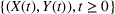
We consider an inventory system with Poisson demand arrivals arising from multiple classes. Restocking epochs are specified by a given sequence. At each epoch, we can place an order for any number of items for immediate delivery. We have to decide the inventory dispensation policy, which determines whether we should satisfy a demand, or reject it, or backlog it until the next restocking epoch. We allow class‐dependent rejection and backlogging costs. We also incorporate holding costs and procurement costs. We obtain the optimal restocking and inventory dispensation policies under the total discounted cost criterion as well as the long‐run average cost criterion. In particular, we develop efficient algorithms to compute the optimal policies (OPs) by decoupling the inventory dispensation policy from the restocking policy. We show that the OP operates as follows: At the restocking epochs, we order up to a fixed base‐stock level. We satisfy the demands from a class if the inventory is above a critical level that depends on the class and time to the next restocking epoch; else we reject or backlog it depending on whether the next restocking epoch is later or earlier than a class‐dependent critical number. The numerical experiments for the stochastic and deterministic interstocking periods are conducted to compare the OPs and costs.
Global supply chain forms the backbone of our modern economy, guiding the flow of trillions of dollars worth of merchandize between the United States and Asia alone. It is an amazingly complex logistics system that manages production, transport, and distribution of a vast array of goods all over the world. For example, an oximeter purchased in the United States is quite likely manufactured in Asia, transported over the ocean in giant container ships, offloaded in a U.S. port, stored in a regional warehouse, and transported by a truck to the final retail store where it waits for an anxious customer to buy it.
In this paper, we focus on the last mile of this global supply chain: from the local warehouse to the retailer. In particular we consider the situation where a large supplier ships many products to many relatively small retailers by trucks. The supplier aggregates the demand for various products from many retailers and sends trucks from its local warehouses to the retailers, restocking their inventories with various products according to their instructions. A single delivery truck may visit many retailers and carry many different products. Since the supply delivery schedule is the result of this aggregation, a single product demand from a single retailer has negligible effect on it. Hence, we assume that the delivery schedule is exogenous and beyond the retailer's control. Given the delivery schedule, the retailer accordingly adjusts the stock‐up levels of its products. The most common situation is where the truck delivery schedule is deterministic and periodic: For example, a supply truck may arrive every Monday, delivering a variety of goods. However, the deterministic schedule can be subject to random variations due to events beyond anyone's control, such as weather, traffic congestion, delivery driver/loader shortages, and delivery truck failures. Thus, we need a probabilistic model of inter‐restocking times. Hence in this paper, we initially consider the general case of the random inter‐restocking times, and then specialize it to the deterministic periodic schedule.
The retailer can manage the random demand in many ways. One of the most common method is inventory rationing. Under this scheme, the retailer segments the demand into multiple classes using various criteria such as profitability, contractual obligations, cost of not satisfying the demand, and the source of the demand. For example, in critical health care products, the retailer may differentiate among the demands from individuals, schools, nursing homes, clinics, hospitals, and so forth. In scarce or expensive products, the retailer may give priority to customers with long‐term contracts over one‐time customers.
Inventory rationing is difficult to justify or implement if the inventory is visible to the customers, as in a regular grocery store. However, it is a feasible strategy when the inventory is invisible to the customers. This can happen in an online setting, where customers place orders online with the retailer. For example, an oximeter retailer can operate an online e‐tail business where hospitals, clinics, and individuals can place online orders and retailer can appropriately ration the inventory, which is invisible to the customers. Inventory rationing can be feasible even in brick and mortar warehouse stores if the front office does not carry any visible inventory. A walk‐in customer talks to a sales clerk in the front office, who looks up the inventory on a computer, and an item is brought out to the customer's car if it is deemed available. We assume that inventory rationing is feasible in this paper.
The retailer has three options when a demand arrives: satisfy it, or reject it, or backlog it (i.e., satisfy it at a later time when fresh inventory is delivered). Of course, the decision depends on its class, the amount of inventory on hand, and the time until the next delivery. For example, a demand for an oximeter maybe satisfied if it is from a hospital, backlogged if it is from a healthcare clinic, and rejected if it is from an individual, based on the current inventory level and when the next restocking is expected. It may make sense not to satisfy a demand from a lower class even if there is inventory on hand so that a future demand from a higher class can be satisfied without delay. Furthermore, if we decide not to satisfy a demand, it may make sense to backlog a demand if the next delivery is close at hand, and reject it otherwise. When a delivery occurs, all existing backlog is cleared, and the inventory is restocked.
We call the policy that determines whether to satisfy/reject/backlog a demand a demand dispensation policy or inventory dispensation policy. Several papers have studied the case where the rejection option is not available. In this case, they study the backlogging policy, that is the policy that determines whether to satisfy/backlog a demand. Several other papers have studied the problem when the backlogging option is not available. In this case they study the inventory rationing policy, that is the policy to determine whether to satisfy/reject a demand. These papers are reviewed in the next section. The policy that determines how much to restock is called the inventory restocking policy. In this paper, we study the joint inventory restocking and demand dispensation policies.
We next discuss the cost models that will help us define the optimal restocking and dispensation policies. When we reject a demand, we incur a class‐dependent lump sum rejection cost. When we backlog a demand, we incur cost at a class‐dependent backlogging rate until the demand is fulfilled at the next restocking epoch. In addition to these costs, there are holding costs and procurement costs. Clearly it makes sense to assume that rejecting or backlogging a demand from a higher class costs more than a similar treatment for a lower class demand. Thus it makes sense to assume that the rejection costs and the backlogging cost rates are monotone functions of class: the higher the class, the higher the backlogging/rejection costs. For example, not satisfying a demand for an oximeter from a hospital has more serious consequences than rejecting an oximeter demand from an individual. Hence, it is natural to assume that rejection cost of oximeter demands from a hospital is greater than that from an individual.
We study the optimal restocking and dispensation policies by formulating the problem as a Markov decision process (MDP). In Section 3 we describe precise cost model and the MDP model assuming that the inter‐restocking times are independent and identically distributed (iid) random variables with a phase‐type distribution. This is not a very restrictive assumption, since any continuous distribution with nonnegative support can be approximated arbitrarily closely by a phase‐type distribution. See Zipkin (1988) for the use of phase‐type distributions for lead times in inventory models. In particular, an Erlang distribution is a phase‐type distribution. Later, in Section 6 we consider the case of deterministic inter‐restocking times, which can be thought as the limiting case of the Erlang distribution.
There are two important features of our model: (i) The restocking intervals are not under our control, hence we do not decide when to restock, only how much to restock after covering the backlog; (ii) If we backlog a demand, it will be cleared at the next restocking epoch, and not earlier. These two features have two important consequences. First, these features simplify the state space of the problem tremendously, and they make the implementation of the resulting policies easy. Typically, when the backlogging costs are class dependent, we need to keep track of the size of the backlog for each class, thus necessitating a multidimensional state space. This makes the analysis intractable and unattractive to implement. However, in our model, we know the distribution of the remaining backlog duration at the time when we decide to backlog a demand. Hence it is possible to set up an MDP without explicitly keeping track of the size of the backlog for each class. This is explained in detail in Section 3. Second, it decouples the demand dispensation policy from the inventory restocking policy. Thus, we can first determine the optimal dispensation policy, and then use it to obtain the optimal restocking policy. This surprising decoupling property leads to an efficient method to compute the optimal dispensation and restocking policies jointly. (See Sections 5 and 6.)
We consider mainly the total discounted cost criterion, and briefly describe the average cost criterion as the limiting case for phase‐type as well as deterministic interstocking times. We show that a base‐stock restocking policy is optimal. The optimal dispensation policy for each class is characterized by a class‐ and time‐dependent critical level and a class‐dependent critical number. We satisfy the demand from a class if the inventory is above the critical level for that class. If the inventory is at or below the critical level at that time, we reject the demand if the time until the next restocking epoch is more than a critical number for that class, and backlog it otherwise. This structure is intuitively appealing and easy to implement.
Although the two features of exogenous stocking times and of fulfilling a backlog only at a restocking time make the problem tractable and produce intuitively appealing policies, they raise two potential concerns. First, we are forced not to fulfill a backorder even if there is ample inventory on hand. We call this the late fulfillment concern. This can lead to suboptimal policies. Second, it can create a seemingly unfair situation where a demand is backlogged now, but a later demand from the same class is satisfied even if no new deliveries have occurred. We call this the unfairness concern. This is clearly not relevant if the customers cannot observe how other customers are treated, even within their own class. We address these two concerns explicitly toward the end of Section 7. There we show by simulation that leftover inventory just before a restocking epoch is small compared to the total demand and hence missing the opportunities for early fulfillment of a backorder will not make a significant difference in the cost. This mitigates the first concern. To address the second concern, we say that a demand is satisfied out‐of‐turn if at least one previous demand from that class is rejected or backlogged during the current interstocking interval. We use simulation to show that although unfair treatment of some early customers is a real possibility under the optimal policy (OP), the fraction of demands satisfied out‐of‐turn in an unfair way is small. Furthermore, if this unfair treatment is absolutely unacceptable, we propose a fair heuristic policy (HP) for the retailer such that once a demand from a class is unsatisfied, no future demand from that class will be satisfied until the next restocking. We compare the performance of this fair heuristic with the possibly unfair OP and show that the two are very close in terms of average costs. Thus, if fairness is a significant issue, the retailer can opt to choose the fair HP. This mitigates the second concern, if it is relevant. This makes a very strong case for the retailers to implement these policies.
We present numerical results and compare the average cost optimal inventory dispensation policies and the restocking policies for two cases: Erlang interstocking times and deterministic interstocking times with the same mean for several parameter combinations. We observe that the OPs for the two cases are surprisingly close over a wide range of parameters.
To the best of our knowledge ours is the only paper that studies the dispensation policies and their optimality. In Section 2, we shall review literature on rationing policies or backlogging policies in multiclass demands. We have not found any papers that deal with dispensation policies and their optimality. Thus, the results of our analysis will help a retailer incorporate all three inventory dispensation alternatives simultaneously, an improvement over the current models that allow only two alternatives.
The remainder of this paper is organized as follows. First we provide a brief review of the related literature and position our paper in the relevant context in Section 2. Section 3 describes the model and introduces the relevant notation. Section 4 gives the main structural results for the total discounted cost criterion with phase‐type inter‐restocking times. In Section 5, we compute the OPs for the total discounted cost criterion and the average cost criterion. We discuss the case with deterministic restocking times in Section 6. Section 7 includes the numerical results and their discussion, as well the fairness and late fulfilment aspects of the OPs. We conclude the paper in Section 8 with an overall summary and discussion.
LITERATURE REVIEW
Our work combines, and is inspired by, two streams of research. The first stream is the classical periodic review inventory models with no set up costs. The second stream is more recent literature on rationing policies (accept or reject demands), or backlogging policies (accept or backlog demands) with multiclass demands. As we mentioned in the previous section, we are not aware of any papers that deal with dispensation policies where there are three options to deal with a demand: accept or backlog or reject. In the following, we explicitly point out what decisions are considered by each paper reviewed here.
The first stream of research in the area of periodic review policies was initiated in the 1950s. Almost all of it is concerned with simple backlogging policies where backlogging occurs when there is no inventory on hand. They typically consider independent demands in successive periods, with backlogging or lost sales, holding costs and backlogging costs, or stock‐out costs, and procurement costs. They consider cases with lead times or without; single demand class or multiple demand classes. A nonexhaustive list of relevant papers is Bellman et al. (1955), Karlin (1958, 1960), Karlin and Scarf (1958), Iglehart and Karlin (1962), Veinott and Wagner (1963, 1965a, 1965b, 1965c), and Bulinskaya (1964a, 1964b). Zipkin (1988) discusses the advantages of using phase‐type distributions to model the demand process and the replenishment lead times in the standard reorder‐point/order‐quantity model of inventory control.
The second stream of research that inspires our work is rationing or backlogging policies with multiple demand classes, which has been studied extensively in the past 20 years. Topkis (1968), Ha (1997, 2000), Kranenburg and van Houtum (2007), and Pang et al. (2014) study the optimal rationing policies (accept/reject demands). We briefly describe their contribution below.
Topkis (1968) considers optimal rationing policies in an inventory system with multiple demand classes and fixed lead times. Ha (1997) considers a single‐item, make‐to‐stock production system with several demand classes for the case of Poisson demands, exponential production lead times, and no backlogging. He shows that the optimal production policy is a base‐stock policy, and the optimal inventory rationing policy is a stock‐reservation policy, which is characterized by a sequence of monotone rationing levels corresponding to different demand classes. Later, Ha (2000) extends his analysis to the case of Erlang distributed production lead times. Kranenburg and van Houtum (2007) consider rationing policies (accept/reject) for multiclass demands such that a demand from a class is satisfied if the inventory level is above a critical level for that class, and rejected otherwise. Pang et al. (2014) study an inventory rationing problem in a lost‐sales make‐to‐stock production system with a fixed production order size and multiple demand classes. They show that the optimal order policy is characterized by a reorder point and the optimal rationing policy is characterized by time‐dependent rationing levels. They then generalize the model to multiple outstanding orders using the Erlang distribution for lead times.
De Véricourt er al. (2000, 2001), Deshpande et al. (2003), Teunter and Haneveld (2008), Fadilo and Bulut (2010), Ghosh et al. (2015), and Shen et al. (2019) discuss the backlogging policies (accept/backlog demands). De Véricourt et al. (2000) study a production system with backorders and a single machine, which produces two types of products. The arrivals of demands are independent Poisson processes and the production lead times are independent and exponentially distributed. They use a two‐dimensional state space to derive OPs.
De Véricourt et al. (2001) compare the performance of the three allocation policies: first come first serve (FCFS), strict priority policy, and multilevel backlogging policy. Under a strict priority policy, demands are satisfied (or backlogged) regardless of their classes, backorders are cleared according to their priorities. Multilevel backlogging policy is similar to the stock‐reservation policy in Ha (1997), which is characterized by a sequence of monotone critical levels. An arriving demand of a certain class is satisfied with the stock if the inventory level is above the critical level of that class, otherwise it is backlogged. They do not allow rejection. Their numerical results show that the multilevel backlogging policy always outperforms the other two policies.
Deshpande et al. (2003) analyze a backlogging policy for a single‐item system in an inventory system with two demand classes, Poisson arrivals and deterministic lead times. They consider a rather intricate backorder fulfilling policy to approximate an intractable OP. Teunter and Haneveld (2008) study inventory systems with two demand classes (critical and noncritical), Poisson demands, fixed lead times, and backorders. They analyze dynamic backlogging strategies where the number of items reserved for critical demand depends on the remaining time until the next order arrives. Fadilo and Bulut (2010) extend the policy in Deshpande et al. (2003) by defining a modified on‐hand inventory level, which captures the information on the status of the outstanding orders. Ghosh et al. (2015) introduce a new class of two‐bin policy for the inventory system with two demand classes, Poisson arrivals, and fixed lead times. This policy assigns two separate bins of inventory for the two demand classes: when the bin intended for the higher demand class is empty, demand from the higher class can still be fulfilled with the inventory from the other bin. Backorders are cleared according to the policy in Deshpande et al. (2003). Shen et al. (2019) consider a periodic‐review, single‐stage inventory system with multiple demand classes and a fixed replenishment lead time. They do not allow rejection. They show that a state‐dependent backlogging‐level policy is optimal for inventory allocation and the optimal backlogging levels are independent of the backorder quantity of each demand class.
Topkis (1968), Pang et al. (2014), and Shen et al. (2019) are most relevant to our paper. However, our work differs from their papers in many aspects. Unlike Topkis (1968), our model considers backlogging as a decision, and considers the infinite horizon case, thus producing simpler policies. Unlike Pang et al. (2014) our model allows backlogging, and chooses the optimal order size. Unlike Shen et al. (2019), our model allows rejection, nondeterministic interstocking times, and needs a much simpler state space. In our paper, we allow three dispensation choices (accept, reject, or backlog) and consider both phase‐type and the deterministic restocking times. We use two‐dimensional state space (regardless of the number of demand classes) and show how to choose the optimal order size using a decoupling approach.
MODEL DESCRIPTION
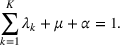
We consider an inventory warehouse that stocks a single product. The demand for this product arises from K distinct sources (called demand classes). Class k demands (
) arrive according to a Poisson process with rate
, and these K demand processes are mutually independent. Suppose we have a positive inventory on hand when a demand arrives. We need to decide whether to satisfy the demand or reject it or backlog it. If we reject a class k demand, it costs
dollars and the inventory on hand remains unchanged. We assume
, that is, demands from class k are more important than those from class
. If we backlog the demand, it costs
per unit time until the demand is fulfilled at the next restocking epoch and the inventory on hand remains unchanged. We do not allow fulfillment before the next restocking epoch. This seems rather inflexible, but it simplifies our analysis. The implications of this modeling assumption are explored in detail in Section 7. We also assume
again indicating that class k demands are more important than class
. When restocking occurs, we fill all backlogged demands. If the inventory on hand is zero when a demand occurs, we cannot satisfy the demand. The only options are to either reject it or backlog it, with the same consequences as before. Thus, the inventory on hand cannot go below zero.
The inventory is restocked at the restocking epochs. Assume that intervals between consecutive restocking epochs (called the restocking intervals) are iid positive random variables. The common distribution of the restocking intervals is phase‐type with M phases with parameters
. This parameterization is slightly different from the standard phase‐type parameters, hence we formally define it below.
Let
be a continuous time Markov chain
on state‐space
that starts in state
with probability
such that
. It stays in state
for an
amount of time and then jumps to state j with probability
,
, or to state 0 with probability
. Let
be an
matrix, and
Then R (or its distribution) is called phase‐type with parameters
.
is called the phase of R at time t.
We assume that
is invertible, so the restocking interval is a random variable with finite expectation. Suppose the phase of the restocking interval is i at time t. Then, after an exp(μ) amount of time, the restocking epoch occurs with probability
, or the phase changes to j with probability
. Phase‐type distributions are dense (see Neuts, 1975) in the set of all distributions of nonnegative random variables. Hence we can approximate any restocking interval distribution by a phase‐type distribution to an arbitrary accuracy. In particular, in Section 6 we will use this to represent a deterministic restocking time distribution as a limit of phase‐type distribution. This flexibility of phase‐type distributions makes them very useful in practice.
When the restocking epoch occurs, the system manager first observes the inventory on hand and all the backlogs, and then decides how much to stock up. All the backlogs are cleared and restocking is done instantly. Let c be the cost of an item, so the cost of ordering x items is
. We assume
to avoid trivialities. There is no additional fixed ordering cost. Let h be the holding cost per item per unit time in the inventory.
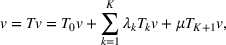
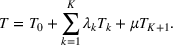
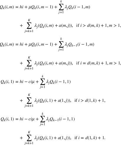
We need to decide the optimal restocking level when the restocking epoch occurs and the optimal inventory dispensation (that is, the acceptance‐backlogging‐rejection decision) when a demand arrives. The objective function is to minimize the total expected discounted cost (with continuous discount factor
) over the infinite time horizon. We will solve this problem by setting it up as an MDP problem.
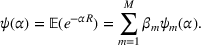
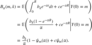
We need the following preliminary result before we present this formulation. Let R be the first restocking epoch as defined in Definition 1, and let
and
Suppose a type k demand occurs at time zero, the restocking time R is in phase
, and we backlog this demand. Let
be the expected total discounted cost connected with this decision. It includes the backlogging cost that is incurred at rate
over [0, R] and the procurement cost c incurred at time R. We have
With this expression we are ready to give the MDP formulation. Let
be the inventory on hand at time t. Let
be the phase of the interrenewal time at time t. Thus, the state space of
is given by
Suppose the state of the system is
. The next event is an arrival of a demand, or a phase change, or a restocking epoch. The next event is an arrival of a demand of type k with rate
, in which case, we have to decide whether to accept or reject or backlog the demand if
, and reject or backlog the demand if
. If the decision is to satisfy the demand, no cost is incurred and the state changes to
. If the decision is to reject the demand, a lump sum cost
is incurred and the state remains unchanged at
. If the decision is to backlog the demand, a lump sum cost
is incurred and the state remains
. Since we pay for the backlogging and procurement cost connected with the backlogging decision up front, we do not need to keep track of the number of backlogged items in the state space. The next event can be a phase change, resulting in a new state
with rate
. Finally, the next event can be a restocking epoch, which occurs with rate
, and if we decide on restocking to level
, a procurement cost
is incurred and the next state is
with probability
.
The problem of finding the optimal dispensation and restocking policy can now be formulated as a continuous‐time MDP. Define
to be the optimal total expected discounted cost over infinite horizon starting in state
. We use the uniformization method to convert this continuous‐time MDP into a discrete‐time MDP as follows. First, we scale the time so that
We will find the following notation useful to simplify the presentation.
Note that
decreases in k. Then we see that the value function v satisfies the following dynamic programming equation:
where
Note that the operators
,
, give the optimal demand dispensation decisions: accept/reject/backlog. In particular, if it is not optimal to accept a type k demand in state
, then it is optimal to reject it if
, and backlog it otherwise. This decision to reject or backlog is independent of i.
The operator
determines the optimal restocking policy. Remember that we have already paid the procurement cost of the backlogged items when we backlogged them (it is included in the cost
), hence we need only to account for the procurement cost of
additional items that we need to bring the inventory on hand up to the level q. This explains why we do not need to keep track of the backlogged items separately in the state space.
We study the structural results for this system in the next section.
MAIN STRUCTURAL RESULTS
We first make the following definition for conciseness:
. Hence the optimal decision when a class k demand arises in state
is to satisfy it if
. If
, it is optimal to either reject it or backlog it, depending on whether the rejection cost
is smaller or the backlogging cost
is smaller. Since
, it follows that
.
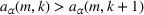
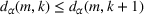
Theorem 2 thus shows that the optimal dispensation policy accepts more demands of type k than of type
. This makes intuitive sense, since type k demands have higher priority than type
demands. The optimal restocking level
does not depend on when (which phase) the restocking opportunity occurs. This is similar to the periodic review inventory policies in the absence of fixed ordering costs. The OP never uses all three options in a given phase for a given class: As the inventory diminishes, it either first satisfies and then rejects all the demands, or it first satisfies and then backlogs all the demands. This is indeed a very nice and unexpected property of the OP.
It is possible that, under the OP, a demand may be rejected or backlogged now, but a later demand from the same class may be satisfied before the next restocking time. This seems unfair to the earlier customer whose demand is not satisfied. We shall discuss this in more detail in Section 7.
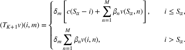
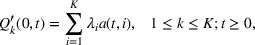
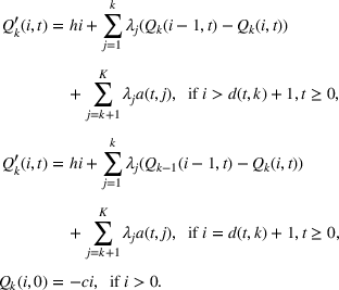
Next we discuss an important decoupling property that leads to an efficient method of computing the optimal restocking policy and the optimal dispensation policy.
COMPUTING THE OP: THE DECOUPLING APPROACH
In this section, we explore an interesting property of this inventory system. We shall show that we can obtain the optimal dispensation policy independently of the restocking policy. Once we have the optimal dispensation policy, it can be used to compute the optimal restocking policy. This two‐step decoupling approach leads to an easier and more efficient method of computing the optimal dispensation thresholds
and optimal restocking level
. We describe the methodology below.
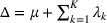
Define a function
that satisfies
where
and
are as before, see (10). An important feature of Equation (16) is the absence of the operator
. This implies that w is essentially describing the dispensation policy.
Define
The main result is given in the following theorem.
it is optimal to reject the demand from class k if
and
it is optimal to backlog the demand from class k if
and
.
See Section B of the Supporting Information.
Computing w using value iteration on Equation (16) is much easier than computing v using Equation (8), since we do not have to do the optimization involved in
at every step of the value iteration. The optimization of the convex function
, which is the expected total discounted cost over (0, R] (see Equation (B‐2)), with respect to x is also almost trivial, resulting in Equation (19). This makes this procedure far more efficient for computing the optimal inventory dispensation and restocking policies. We end this section with a brief comment about the average cost OPs.
Average cost OP
Since the structure of the optimal restocking policy and the optimal dispensation policy as described in Theorem 3 holds for all
, it is clear that the same holds for the long‐run average cost case. We include the details in Section C of the Supporting Information. We assume that the phases are indexed so that
where
and define
Note that
need not be monotone in k. It now follows that the policy that minimizes the long‐run expected cost per unit time is described by critical numbers S and
as follows: It stocks up to S at the restocking epochs, and in state
satisfies a demand from class k in state
if
;
rejects a demand from class k if
and
;
backlogs a demand from class k if
and
.
We can show that
in the average cost case, that is, the demands from class 1 are never rejected if there is inventory on hand. The formal proof is included in Section C of the Supporting Information. Note that this statement may not be valid in the discounted cost case.
We shall use the average cost policy to illustrate the numerical results in Section 7.
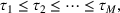
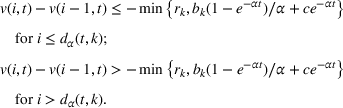
DETERMINISTIC RESTOCKING TIMES
In this section, we consider the case where the restocking intervals are constant, equal to τ. As before, we consider the discounted cost case with continuous discount factor α. Suppose the current inventory level is i and the next restocking epoch is t time units into the future. Let
) be the expected total discounted holding and rejection/backlogging cost over the next t time units. For reasons that will become clear later, we assume that leftover inventory at the restocking epoch (
) is disposed off at price c per item, and this is included in the definition of v. Let
be derivative of v with respect to t. The following theorem gives the equations satisfied by v.
For
and
,
with boundary conditions
See Section D of the Supporting Information.
Note that τ does not play any role in the above equations. Hence we can replace
in the above equations by
. The next theorem gives the main structural property of v.
is convex in i for each
.
Follows from the proofs of Theorem EC.1 in the Supporting Information and Theorem 4.
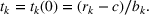
Now we assume that
(we have already assumed that
), since otherwise the rejection decision will always be inferior to backlogging. Then the following quantity is well defined and positive:
Now define
Consider a policy π that operates as follows: It restocks the inventory up to
at each restocking epoch. In state
, it
satisfies class k demands if
,
rejects class k demands if
and
,
backlogs class k demands if
and
.
The next theorem gives the optimality of this policy π.
Policy π minimizes the expected discounted total cost over infinite horizon. Further
is nondecreasing in k.
From the results of the phase‐type model, we know that the OP is to restock up to x at each restocking epoch. We see that the expected total discounted cost of such a policy in the deterministic restocking interval case is given by
Strictly speaking, the procurement cost at time τ is
minus c times the inventory at time τ. However, the cost c times the inventory at time τ is already accounted for by the boundary condition in Equation (24). Hence we are left with the term
Thus, by (25) and (27), it is optimal to reject a demand of class k in state
if
and
, to backlog a demand of class k in state
if
and
, and to satisfy class k demands in state
if
.
Finally,
is nondecreasing in k is a direct consequence of convexity of
in i for each fixed t and the fact that
is decreasing in k.
We end this section with a brief comment on the average cost OP in the case of deterministic restocking times.
Average cost OP
Notice that Equations (22)–(24) and (28) remain valid when
. In this case,
gives the long‐run average cost if the inventory is restocked to level x at every restocking epoch. Then Equation (25) reduces to
Let
, and
. We see that the policy that minimizes the long‐run expected cost per unit time operates as follows: It restocks the inventory up to
at each restocking epoch. In state
, it
satisfies class k demands if
,
rejects class k demands if
and
,
backlogs class k demands if
and
.
Analogous to the Erlang case in Section 5.1, we can show that
. That is, the average cost OP satisfies class 1 demands if the inventory on hand is positive. This is expected intuitively. We omit the formal proof.
We shall illustrate the numerical results in the next section using the average cost OP.
NUMERICAL RESULTS
In this section, we demonstrate the structure of the OP with numerical experiments using the long‐run average cost setup. To be specific, we consider two distributions for the restocking times:
Case E: Erlang (
).
Case D: Deterministic with mean τ.
We first explain how we compute the OP for Case E based on Section C of the Supporting Information. We compute
, using Equations (C‐6) and (C‐7). They reduce to the following (with
):
These can be solved recursively easily, without resorting to iterative algorithms. Then we use Equation (C‐9) to compute
which is the long‐run average cost if we stock up to i at every restocking epoch. Then we use Theorem EC.1 to compute the optimal restocking level S, the optimal control thresholds
, the optimal backlogging levels
, and the optimal cost per unit time
.
For Case D, we numerically solve Equations (22)–(24) with
, using a simple discretization of time using step size = 0.1. Then we compute the long‐run average cost as (using the same notation as in Case E)
We follow the procedure given at the end of Section 6 to compute the optimal restocking level
, the functions
for
, the parameters
, and the optimal cost per unit time
.
Effect of model parameters
In this subsection, we study the effect of model parameters on the performance of the policy for a system with
demand classes. Class 1 has the highest priority and class 3 has the lowest. The total arrival rate of demands is λ. Of this, 20% are class 1 demands, 30% are class 2 demands, and 50% are class 3 demands. Thus, the arrival rates of individual classes are
We fix rejection costs as
,
and
, and backorder costs as
,
, and
. We assume the holding cost rate is h and the procurement cost is
per item. We consider nine scenarios by varying λ and h as follows:
We can think of λ as the size of the system (larger λ representing larger system), and h as the relative contribution of holding cost and rejection cost to the total cost per unit time (larger h implying more expensive inventory to hold). We consider the following two cases:
Case E: Erlang (
) restocking times with
,
;
Case D: Deterministic restocking times with
.
Note that both restocking times have the same mean of 100 so that we can compare the results. However, the standard deviation in the Erlang case is 31.6, while that in the deterministic case is zero. These values of the system parameters are used throughout this section.
We describe the numerical results below for
and
. We first plot long‐run average cost function
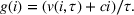
in Figure 1. Figure 1a shows Case E and Figure 1b shows Case D. We see that for both cases, the long‐run average cost is a convex function of i and is minimized at
for Case E and
for Case D, which implies that the optimal restocking level is
for Case E and
for Case D. The convexity is theoretically proven in Sections 5 and 6. The optimal long‐run average cost is 7.9830 for Case E and 7.2052 for Case D. We would expect the optimal long‐run average costs and the restocking level for Case D to be lower than those for Case E due to higher variability in Case E. This is consistent with the observation. However, the closeness of the optimal restocking levels and their long‐run average costs is surprising and useful.
Long‐run average costs: (a) Erlang case, (b) deterministic case
We study the demand dispensation policy next. Recall that for Case E, when
with respect to t for Case D in Figure 2b. We set the upper limit of i‐axis as their optimal restocking levels. Note that in Figure 2a,b we also separate the demand rejection and back‐order regions by
for Case E and by
for Case D. We can see that Figure 2a is similar to Figure 2b. This implies that the optimal demand dispensation policies for Case E are close to those in Case D. We discuss them in more detail below.
is nondecreasing in k, which is consistent with Theorem 6. Also, from Figure 2b we see that
,
, and
, which are consistent with Equation (31). Note that
is also close to
, the expected restocking time in phase
(namely, 70, 60, and 50). For Case D, the optimal dispensing policy is as follows:
for class 1, satisfy the demands when
, reject the demands when
and
, backlog the demands if
and
;
for class 2, satisfy the demands when
, reject the demands when
and
, backlog the demands if
and
;
for class 3, satisfy the demands when
, reject the demands when
and
, backlog the demands if
and
.
Next we report the extensive numerical experimentation for the nine scenarios as mentioned in the beginning of this subsection, using three values of h and three values of λ. Of these nine scenarios, we have reported the scenario
and
in detail above. The corresponding figures and parameters of the OPs for the other eight scenarios are given in Section F of the Supporting Information. As expected, we see that, in both Cases E and D, the d curves move up as λ increases, and move down as h increases. This is consistent with our intuition: We should stock more and reject fewer demands if the demand is high, and holding cost is low.
The summary of these nine scenarios is given in Tables 1 and 2 for Cases E and D, respectively. We shall explore the table entries in more detail below.
Performance measures of the optimal policy: Erlang case
h
λ
g
S
0.05
0.5
6.8705
52
0.9570
0.0000
0.0430
0.9405
0.0009
0.0586
0.7968
0.0546
0.1486
0.05
1
13.6212
102
0.9595
0
0.0405
0.9349
0.0008
0.0643
0.7892
0.0556
0.1552
0.05
2.5
33.8672
254
0.9629
0
0.0371
0.9346
0.0008
0.0646
0.7933
0.0519
0.1548
0.1
0.5
7.9830
43
0.9173
0.0001
0.0826
0.8844
0.0035
0.1121
0.6545
0.1206
0.2249
0.1
1
15.7823
84
0.9252
0.0001
0.0747
0.8761
0.0033
0.1206
0.6430
0.1204
0.2366
0.1
2.5
39.1706
209
0.9288
0.0000
0.0712
0.8749
0.0033
0.1218
0.6420
0.1185
0.2395
0.2
0.5
9.5196
33
0.8516
0.0005
0.1479
0.7802
0.0165
0.2033
0.4534
0.2348
0.3118
0.2
1
18.7768
66
0.8646
0.0003
0.1351
0.7752
0.0141
0.2107
0.4578
0.2248
0.3174
0.2
2.5
46.5278
164
0.8688
0.0002
0.1310
0.7745
0.0129
0.2126
0.4526
0.2266
0.3208
Performance measures of the optimal policy: Deterministic case
h
λ
g
S
0.05
0.5
6.2824
45
0.9756
0
0.0244
0.9560
0
0.0440
0.7975
0.0026
0.1999
0.05
1
12.3823
88
0.9705
0
0.0295
0.9489
0
0.0511
0.7917
0.0004
0.2079
0.05
2.5
30.6408
219
0.9682
0
0.0318
0.9418
0
0.0582
0.7982
0
0.2018
0.1
0.5
7.2052
40
0.9459
0
0.0541
0.9108
0
0.0892
0.6676
0.0166
0.3158
0.1
1
14.1667
79
0.9402
0
0.0598
0.8965
0
0.1035
0.6669
0.0048
0.3283
0.1
2.5
35.0167
196
0.9348
0
0.0652
0.8831
0
0.1169
0.6642
0.0004
0.3354
0.2
0.5
8.5923
32
0.8816
0
0.1184
0.8125
0
0.1875
0.4459
0.1014
0.4527
0.2
1
16.8867
65
0.8796
0
0.1204
0.8002
0
0.1998
0.4707
0.0640
0.4653
0.2
2.5
41.7422
163
0.8775
0
0.1225
0.7868
0
0.2132
0.4822
0.0397
0.4781
To begin with, consider the optimal restocking level S given by the fourth column in these two tables. We see that the optimal S increases with λ and decreases with h. This is consistent with our expectation: We should stock more inventory if the expected demand is higher, and if it costs less to stock it. We see that the optimal restocking levels in Case D are consistently lower than those in Case E. This is an expected consequence of the higher variability in Case E, but their closeness is surprising. It is instructive to compare the optimal S values to the expected demand
in one interstocking interval: 50 in the small system (
), 100 in the medium size system (
), and 250 in the large system (
). We define “relative stocking level” as
, which may be greater than 100% or less than 100%. We see that the relative stocking level in Case E is over 100% when
, around 90% when
, and around 67% when
. They are slightly lower in Case D. These are representative levels in real‐life operations.
The optimal long‐run average cost appears in the third column of Tables 1 and 2. As with optimal restocking level, the average cost is higher in Case E compared to that in Case D, manifesting the effect of higher variability. It increases as the demand increases and the holding cost increases, as expected.
Now we study other performance measures of the OP. Let
,
, and
be the fractions of demands from class k that are satisfied, rejected, and backlogged, respectively, under the OP. We use simulation with 10,000 replications to estimate these fractions, and present the results in the last nine columns of Tables 1 and 2. From these two tables we find that the OP does show preferential treatment for class 1 customers: The satisfaction fractions decrease with the class index, and the rejection and backlogging fractions increase with the class index, in all the scenarios. This is what the OP is designed to do.
Next we consider the trends with respect to the holding costs. We see that for both Cases E and D and for all scenarios, the satisfaction fractions diminish as h increases. This is mainly because the optimal restocking levels decrease with h. The OP concludes that it is better to incur rejection costs rather than holding costs. In contrast, rejection and backlogging fractions increase with h.
Finally we consider the trends with respect to the overall arrival parameter λ. Here, the situation is not so clear‐cut. In Case E, the satisfaction fractions of class 1 increase with λ, and the rejection and backlogging fractions decrease with λ. For other classes, the satisfaction, rejection, and backlogging fractions can show minor nonmonotonic behavior with λ! The story is similar in Case D. This is a manifestation of the intricate roles played by various cost parameters in the model. It is interesting to see the same trends in both the Erlang and deterministic cases. Since these two results are computed by two entirely different computer simulation programs, we can confidently conclude that this nonmonotonicity, although minor, is a real phenomenon, and not an artifact of the random nature of simulation results.
It is of interest to study the performance of the system by varying other parameters of the system, namely, the rejection costs, the backorder costs, or the traffic mix among the classes. The performance of the system behaves as expected as these parameters change. We have included the results in Tables EC.1 through EC.6 in Section G of the Supporting Information, obtained by changing one set of parameters at a time. Formally,
keep other parameters unchanged and change only rejection costs from [100, 50, 20] to [100, 80, 50]: Tables EC.1 and EC.2;
keep other parameters unchanged and change only backorder costs from [1.4, .7, .2] to [1, .8, .3]: Tables EC.3 and EC.4;
keep other parameters unchanged and change only traffic mix from λ[.2, .3, .5] to λ[.1, .2, .7]: Tables EC.5 and EC.6.
First consider the results in Tables EC.1 and EC.2. Here we have kept all other parameters unchanged, but have increased the rejection costs from [100, 50, 20] to [100, 80, 50]. Thus, we expect the rejection fractions for the three classes to go down. This is indeed observed in Table EC.1 for Case E, and in Table EC.2 for Case D. It is worth noticing that although the rejection costs for classes 2 and 3 went up substantially, the optimal cost per unit time went up only marginally. This is the result of the fact that the policy makers have many decision levers that can be pulled to make the system behave well.
Next consider the results in Tables EC.3 (Case E) and EC.4 (Case D). These relate to the scenario where all other parameters are unchanged, except the backorder costs have been changed from [1.4, 0.7, 0.2] to [1, 0.8, 0.3]. Thus, the backorder cost for class 1 is reduced, and for classes 2 and 3 has increased. Thus, we expect the backlogging fractions for class 1 to increase and those for classes 2 and 3 to decrease. This is indeed observed from comparing these two tables to Tables 1 and 2. A surprising behavior is that the optimal restocking levels and optimal costs change only marginally in response to these changes in the backorder costs.
Finally consider the results in Tables EC.5 and EC.6. Here we keep all parameters same but change the traffic mix, class 1 traffic reduces from 20% to 10%, class 2 traffic reduces from 30% to 20%, and class 3 traffic increases from 50% to 70%. Since more of the traffic is lowest priority one, we expect to need lower restocking levels and lower costs per unit time. This is indeed observed when comparing Table EC.5 to Table 1 (Case E), and Table EC.6 to Table 2 (Case D). The restocking levels decrease appreciably, and costs also go down. As before, the performances in the Erlang and deterministic cases are similar.
We have consistently observed that the results of Cases E and D are fairly close. This is surprising since the variance of the interstocking time in Case D is zero, while that in Case E is significant. This higher variance mainly explains the difference in all the performance measures as discussed in appropriate places in this subsection.
Next we address the two potential concerns related to the OPs: late fulfillment of backorders and unfair treatment of early customers, in the following two subsections.
Late fulfillment
Recall that under our policy, once a demand is backlogged, it can be fulfilled only at the next restocking epoch. Again, this is not an issue since the inventory is not visible to the customers. But it is less than optimal if we encounter large on‐hand inventory and large number of backorders simultaneously. From Tables 1 and 2, we see that significant fraction of the demands can indeed be backlogged, especially in large systems. So we study the ending inventory L, that is, the level of on‐hand inventory just before the restocking epoch. A large L would imply more missed opportunities of fulfilling the backorders early, while a small L would mean relatively few such missed opportunities.
We simulate the OP to estimate
. We use 10,000 replications for each scenario. The results are presented in Table 3. We see that expected leftover inventory is much lower in the deterministic case than in the Erlang case. However, the difference
is about the same in both cases. This is just a manifestation of the effect of variability in the Erlang case, which forces the optimal restocking level S higher. We see that the percentage of the starting inventory that is leftover in the end in Case E varies from about 4% (for
) to about 16% (for
) and about 0% to 2% in Case D. Thus, especially in Case D, we are not missing any appreciable number of early fulfilment opportunities. We have also included the expected number of backlogged orders
in each scenario. Note that in all scenarios,
is much larger than
, implying that we cannot avoid many of the backorders even if we allow early fulfilment. This shows the extra cost that we might be paying for the simplicity of the optimal dispensation policy. It misses more early fulfilment opportunities in the lower holding cost setting as compared to the higher holding cost settings. But the cost saving implied by early fulfilment will be lower if the holding cost is low. This mitigates the concern around late fulfillment.
Ending inventory and backlog
Erlang
Deterministic
h
λ
0.05
0.5
8.4167
0.1619
5.024
1.0541
0.0234
5.902
0.05
1
15.2528
0.1495
10.499
0.5627
0.0064
12.518
0.05
2.5
35.8778
0.1413
26.063
0.1234
0.0006
31.180
0.1
0.5
4.1706
0.0970
8.130
0.2555
0.0064
9.774
0.1
1
7.1083
0.0846
16.942
0.0610
0.0008
20.716
0.1
2.5
16.5433
0.0792
42.640
0.0030
0.0000
53.953
0.2
0.5
1.4588
0.0442
12.324
0.0131
0.0004
15.314
0.2
1
2.5303
0.0383
24.893
0.0006
0.0000
31.667
0.2
2.5
5.4461
0.0332
62.595
0
0
81.878
Unfairness
Now we address the potential for unfair treatment of the early customers. Under the OP, it is possible that a demand is rejected/bakordered now, but a later demand from the same class is satisfied, even though no restocking has occurred. For example, consider Figure 2a. Suppose the system state is
. If a demand from class 3 arrives in this state it will be rejected under the OP. Now, it is possible that at a later time the state changes to
. If a demand from class 3 arrives now, it will be satisfied. This seems unfair, and may cause resentment on part of the early customers, especially if the customers can tell how other customers are getting treated.
We develop two indices to quantify how pervasive this situation is by defining an unfairness index. We say that an order is satisfied out‐of‐turn if at least one previous order from that class is rejected or backlogged during the current interstocking interval. Let
be the number of orders from class k that are satisfied out‐of‐turn during an interstocking interval under the OP, and
be the number of unsatisfied orders (i.e., they are rejected or backlogged) from class k during one interstocking interval. The expected demand of type k during an interstocking interval is
, where τ is the expected interstocking interval. Define the following two unfairness indices:
We see that
is the fraction of total demands of class k that are satisfied out‐of‐turn, while
is the number of demands that are satisfied out‐of‐turn per unsatisfied demand. The denominator of the first index is independent of the dispensation policy, while that in the second depends on it. Thus, in some sense, the second index is more sensitive to the dispensation policy. The second index is expected to be higher than the first, and measures a different aspect of unfairness. The higher the values of these indices, the more pronounced the unfairness of the policy.
We estimate the unfairness index for each class by simulating 10,000 replications. Table 4 displays the unfairness indices for the three classes for the Eralng case and the deterministic case for three values of h and three values of λ. From the table we see that the unfair events, although possible, are not common.
Unfairness indices
Erlang
Deterministic
h
λ
ρ2
ρ3
ρ2
ρ3
0.05
0.5
0
0.0017
0.0285
0.0202
0.0995
0
0.0013
0.0303
0.0071
0.0348
0.05
1
0
0.0012
0.0177
0.0233
0.1103
0
0.0021
0.0403
0.0040
0.0190
0.05
2.5
0
0.0011
0.0173
0.0227
0.1099
0
0.0017
0.0299
0.0017
0.0085
0.1
0.5
0
0.0029
0.0247
0.0350
0.1015
0
0.0036
0.0405
0.0089
0.0268
0.1
1
0
0.0026
0.0211
0.0357
0.0999
0
0.0039
0.0381
0.0043
0.0130
0.1
2.5
0
0.0022
0.0178
0.0365
0.1021
0
0.0020
0.0175
0.0014
0.0041
0.2
0.5
0
0.0067
0.0307
0.0423
0.0774
0
0.0077
0.0410
0.0115
0.0207
0.2
1
0
0.0049
0.0219
0.0398
0.0734
0
0.0046
0.0230
0.0057
0.0108
0.2
2.5
0
0.0040
0.0180
0.0424
0.0774
0
0.0019
0.0089
0.0024
0.0047
From the table we see that both the unfairness indices are quite small: The maximum ρ is about 4.25% for class 3 in the Erlang case when
and
and the maximum
is about 11% for class 3 when
and
. Class 1 customers never face this unfair situation. The unfairness is not monotone in any parameter like h, or λ or even the class index k. For example, in many scenarios, class 3 can fare slightly better than class 2! This is not surprising, since unfairness is a function of many parameters. The situation in Case D is similar with lower values for the indices in all the scenarios. The main takeaway is that unfairness is manageable and not too detrimental.
Fair HP
Next we explore a HP that explicitly avoids unfairness. We first describe it for the Erlang case. The policy for the deterministic case is similar. The HP follows the OP for each class k until the OP rejects or backlogs a demand from class k. From then on the HP rejects a demand from class k in phase m if
and backlogs it otherwise. Thus, HP will never satisfy a demand from class k in an out‐of‐turn way. We show how to compute long‐run average cost of this HP.
Let
be the expected total cost under HP until the next restocking epoch starting in state
, and assuming that demands from classes 1 through k are satisfied (
) and others are postponed. Since in state (0, m) none of the demands are satisfied, we see that
where
We define
for
for notational convenience. The other Q quantities are computed recursively as follows (assuming
):
If
is not defined in the above equations, we set it to zero. These quantities can be computed recursively easily. Let S be as in Theorem EC.1. The long‐run average cost of this HP is
The HP for Erlang case can be extended to phase‐type case, which is discussed in Section E of the Supporting Information.
For the deterministic case, we define
as the expected total cost under HP until the next restocking epoch starting in state
, and assuming that demands from classes 1 through k are satisfied (
) and others are postponed. Since in state (0, t) none of the demands are satisfied, we see that
where
The other Q quantities are computed recursively as follows:
If
is not defined in the above equations, we set it to zero.
The above quantities can be computed recursively by simple numerical methods. Let
be as in the average cost part at the end of Section 6. The long‐run average cost of this HP is
We present the average cost for the HP and the OP for the Erlang and the deterministic cases in Table 5 for the three values of h and λ as in the previous tables.
HP and OP costs in the Erlang and deterministic cases
h
λ
g(HP, Erl)
g(OP, Erl)
g(HP, Det)
g(OP, Det)
0.05
0.5
6.8946
6.8705
6.2933
6.2824
0.05
1
13.6703
13.6212
12.3931
12.3823
0.05
2.5
33.9719
33.8672
30.6499
30.6408
0.1
0.5
8.0332
7.9830
7.2275
7.2052
0.1
1
15.8705
15.7823
14.1850
14.1667
0.1
2.5
39.3699
39.1706
35.0281
35.0167
0.2
0.5
9.5982
9.5196
8.6406
8.5923
0.2
1
18.9031
18.7768
16.9218
16.8867
0.2
2.5
46.8058
46.5278
41.7599
41.7422
From this table, we see that the average cost of the HP is very close to that of the OP. Clearly, more analytical and numerical work is needed (say with more classes of customers) to explore whether this conclusion holds in general. Thus, if the unfairness is a serious concern, we believe the retailer can use the HP instead of OP without losing much in terms of performance.
CONCLUSIONS
In this paper, we study the optimal restocking and dispensation policies in an inventory system with K demand classes with rejection and backlogging. The restocking intervals are iid random variables beyond the control of the decision maker. We consider the discounted cost and the average cost policies with phase‐type inter‐restocking intervals, and also with deterministic inter‐restocking intervals. For the phase‐type case, we show that the optimal restocking policy is characterized by a restocking level S, and the optimal dispensation policy is characterized by control limits
and
. We develop a decoupling method of computing these policy parameters, and show that
is monotone in k.
For the deterministic case, we show that the structure of the OPs remains same as in the phase‐type model, and is characterized by a restocking level S, control functions
, and critical numbers
. We show that the properties of
are similar to those of
.
Our numerical study compares the Erlang case with the deterministic case, both having the same mean inter‐restocking time. We find that with the same expected restocking times, the optimal restocking and dispensation policies for the two cases are quite close. The optimal long‐run average costs for the deterministic cases are consistently slightly lower than the corresponding Erlang cases. This is to be expected since the Erlang distribution has more variability than the deterministic case. We have been unable to show the monotonicity of
in m for the Erlang case, or
in t for the deterministic case, although we have always observed this monotonicity in all our numerical experiments. We leave this as a topic for future research.
Our OP fulfills the backorders only at restocking epochs. We show by simulation that the opportunities for early fulfillment of backorders are not large enough to justify more complex dispensation policies. Thus, the simplicity of the OP outweighs the slight cost savings that may be achieved by fulfilling some backorders early.
We also consider the possibility of unfair treatment of early customers. We find that this occurs with fairly low frequency in the numerical experiments conducted and reported here. We also suggest a fair HP that is a simple modification of the OP that ensures that such unfairness will never occur. We find the cost performance of the fair heuristic policy is almost the same as the OP based on our numerical experimentation with three demand classes. A further detailed analysis is needed to provide bounds on the difference between performances of the fair heuristic policy and the OP under different parameters. We believe that, based on our numerical experimentation, the fair heuristic will be a good policy to follow in practice.
Footnotes
ACKNOWLEDGMENTS
The authors would like to thank the anonymous senior editor and reviewers for valuable comments that improved the paper considerably, in particular, suggestions to incorporate class‐dependent backlogging/rejection costs, to explore the possibility of decoupling the dispensation decision from the restocking decision, and to address the concerns about late fulfillment of backorders, and potential unfair treatment of early customers.
References
1.
BellmanR.GlicksbergI.GrossO. (1955). On the optimal inventory equation. Management Science, 2(1), 83–104.
2.
BulinskayaE. (1964). Some results concerning optimum inventory policies. Theory of Probability and Its Applications, 9(3), 389–403.
3.
BulinskayaE. (1964). Steady‐state solutions in problems of optimum inventory control. Theory of Probability and Its Applications, 9(3), 502–507.
4.
De VéricourtF.KaraesmenF.DalleryY. (2000). Dynamic scheduling in a make‐to‐stock system: A partial characterization of optimal policies. Operations Research, 48(5), 811–819.
5.
De VéricourtF.KaraesmenF.DalleryY. (2001). Assessing the benefits of different stock‐allocation policies for a make‐to‐stock production System. Manufacturing & Service Operations Management, 3(2), 105–121.
6.
DeshpandeV.CohenM. A.DonohueK. (2003). A threshold inventory rationing policy for service‐differentiated demand classes. Management Science, 49(6), 683–703.
7.
FadiloğluM. M.BulutÖ. (2010). A dynamic rationing policy for continuous‐review inventory systems. European Journal of Operational Research, 202(3), 675–685.
8.
GhoshS.PiplaniR.ViswanathanS. (2015). A new class of multi‐bin policies for inventory systems with differentiated demand classes. Production and Operations Management, 24(5), 840–850.
9.
HaA. Y. (1997). Inventory rationing in a make‐to‐stock production system with several demand classes and lost sales. Management Science, 43(8), 1093–1103.
10.
HaA. Y. (2000). Stock rationing in an make‐to‐stock queue. Management Science, 46(1), 77–87.
11.
IglehartD.KarlinS. (1962). Optimal policy for dynamic inventory process with nonstationary stochastic demands. In KarlinS.ScarfH. (Eds.), Studies in applied probability and management science. Stanford University Press127147.
12.
KarlinS. (1958). Optimal Inventory Policy for the Arrow‐Harris‐Marschak dynamic model. In KarlinS.ScarfH. (Eds.), Studies in the mathematical theory of inventory and production. Stanford University Press, 135–154.
KarlinS.ScarfH. (1958). Inventory models of the Arrow‐Harris‐Marschak type with time lag. In KarlinS.ScarfH. (Eds.), Studies in the mathematical theory of inventory and production. Stanford University Press, 155178.
15.
KranenburgA. A.vanHoutumG. J. (2007). Cost optimization in the lost sales inventory model with multiple demand classes. Operations Research Letters, 35(4), 493–502.
16.
NeutsM. F. (1975). Probability distributions of phase type. In R. Holvoet (Ed.), Liber Amicorum Prof. Emeritus H. Florin (pp. 173–206). University of Louvain.
17.
PangZ.ShenH.ChengT. (2014). Inventory rationing in a make‐to‐stock system with batch production and lost sales. Production and Operations Management, 23(10), 1243–1257.
18.
ShenX.BaoL.YuY.HuaZ. (2019). Managing supply chains with expediting and multiple demand classes. Production and Operations Management, 28(5), 1129–1148.
19.
TeunterR. H.HaneveldW. K. K. (2008). Dynamic inventory rationing strategies for inventory systems with two demand classes, Poisson demand and backordering. European Journal of Operational Research, 190(1), 156–178.
20.
TopkisD. M. (1968). Optimal ordering and rationing policies in a non‐stationary dynamic inventory model with n demand classes. Management Science, 15(3), 160–176.
21.
VeinottA.WagnerH. (1963). Optimal stockage policies with nonstationary stochastic demands. In ScarfH.GilfordD.ShellyM. (Eds.), Multistage inventory models and techniques. Stanford University Press, 85–115.
22.
VeinottA.WagnerH. (1965). The optimal inventory policy for batch ordering. Operations Research, 13(3), 424–432.
23.
VeinottA.WagnerH. (1965). Optimal policy for a multi‐product, dynamic non‐stationary inventory problem. Management Science, 12(3), 206–222.
24.
VeinottA.WagnerH. (1965). Optimal policy in a dynamic, single product, non‐stationary inventory model with several demand classes. Operations Research, 13(5), 761–778.
25.
ZipkinP. (1988). The use of phase‐type distributions in inventory‐control models. Naval Research Logistics, 35(2), 247–257.
Supplementary Material
Please find the following supplemental material available below.
For Open Access articles published under a Creative Commons License, all supplemental material carries the same license as the article it is associated with.
For non-Open Access articles published, all supplemental material carries a non-exclusive license, and permission requests for re-use of supplemental material or any part of supplemental material shall be sent directly to the copyright owner as specified in the copyright notice associated with the article.