Preparedness with a system integrating inventory,capacity,and capability for future pandemics and other disasters

Abstract

The chaotic response of the US Strategic National Stockpile to COVID‐19 during 2020 highlighted the inadequacy of the inventory‐based approaches to disaster response. This paper examines the integration of stockpile inventory, backup capacity, and standby capability to meet the disaster‐related surge in demand in the future. We present a two‐period model of such an integrated system for consumable items with uncertain demand that follows a general probability distribution. Our model incorporates standby capability in period 1 that can be converted to additional capacity for use in period 2, with the conversion yield being deterministic or stochastic. Our main results are: (1) Adding capacity in addition to inventory is beneficial only when the capacity reservation‐related costs are relatively lower than the inventory‐related costs. In this case, adding capacity will decrease the inventory needed in both periods, the shortfall probability, and the total expected cost. (2) Adding capability in period 1 is cost‐effective only when the ratio of capability‐development cost to conversion yield is lower than the capacity reservation cost. In this case, investing in capability results in less inventory and less reserved capacity in period 2. (3) Higher uncertainty in capability conversion yield reduces the attraction of developing capability in period 1. Consequently, less capability would be developed in period 1, while more inventory and capacity would be needed in period 2 in the face of a higher shortfall probability.

Keywords

backup capacity pandemic and disaster response standby capability stockpile inventory

INTRODUCTION

Many countries and organizations maintain strategically located warehouses to supply relief items to beneficiaries rapidly while responding to a disaster. For example, United Nations Humanitarian Response Depot is a network of depots in strategic locations around the world to transport emergency relief items on behalf of member humanitarian organizations, enabling response times of 24–48 h. Similarly, the US Department of Health and Human Services maintains the Strategic National Stockpile (SNS) for preparedness and response. The SNS can ship a broad range of consumable pharmaceuticals and medical supplies from strategically located warehouses throughout the United States to any state in 50‐ton containers within 12 h in case of a public health emergency. However, COVID‐19 exposed the shortcomings of the current inventory‐based national stockpiles of personal protection equipment (PPE) and other critical items in the United States and other countries (Togoh, 2020). Makeshift efforts to tap into the domestic manufacturing capabilities as a backup in 2020 also floundered (Sodhi & Tang, 2021a).

It is, therefore, necessary to rethink preparedness for future disruptions beyond stockpiles. US President Biden's review of the domestic supply chain recognizes the structural weaknesses of domestic supply chains. The review suggests the need to improve stockpile policy, establish domestic production capacity, and develop R&D capability for developing future products. These findings are consistent with industry reports issued by consultancies BCG and McKinsey, supporting the use of backup capacity and the development of new supply chain capabilities (Alicke et al., 2020; Aylor et al., 2020).

Going beyond stockpiles, there is a need to identify and reserve backup domestic manufacturing capacity and develop domestic manufacturing and related capabilities. Having these would be critical during a global pandemic because foreign suppliers may not even be allowed to export products like N95 masks or even components like melt‐blown fabric for producing N95 masks (Sodhi et al., 2021). The government and industry consortia can create capability in different forms such as manufacturing, engineering, research, and development as industrial commons (Pisano & Shih, 2009).

The White House report from the review and various industry reports call for inventory, capacity, and capability, but do not recognize the synergies from coordinating these three resources proactively.¹ We go one step further by examining the implications of integrating inventory, capacity, and capability for preparedness. Such an integrated system with “optimal” levels of each resource prior to a disaster can facilitate a three‐tiered response: (1) Public health authorities would use inventory at first for, say, a viral epidemic in line with current practice. (2) If the epidemic turned into a pandemic,² the authorities would authorize using backup capacity to produce more. (3) And, if the number of affected people kept growing, the government would authorize converting capability into production capacity. Such a three‐tiered response could be more cost‐effective than the one based on inventory alone. Sodhi and Tang (2021b) discuss the idea of such a three‐tiered response system as especially suitable for rare emergencies like pandemics.

This paper presents a two‐period model to capture the time delay in converting capability into production capacity. In this model, the decision to develop capability is made in the first period and this capability becomes available as additional capacity in the second period. The demand created by a disaster for critical consumable items in each period is uncertain, and we assume it follows a general distribution.

Our analysis appears in four steps. First, we consider an inventory‐based system without any backup capacity or standby capability. Second, we analyze a capacity‐based system with backup capacity added to the inventory. Third, we present the fully integrated capability‐based system incorporating standby capability with deterministic conversion yield for converting capability to capacity, which allows the capability decision in period 1 to create additional capacity in period 2. Our main results integrate all three resources. Finally, we extend the integrated capability‐based model to allow for uncertain conversion from capability in period 1 to capacity in period 2. We obtain analytical results for a special case when the capability conversion yield follows a two‐point distribution, where one point refers to the conversion failing altogether. We also obtain consistent numerical results for the general two‐point distribution case.

Our results are threefold: First, adding backup capacity to stockpile inventory lowers the inventory needed, the shortfall probability, and the total expected cost as long as the unit reservation and exercise costs of the capacity are below a certain threshold. Second, developing capability in period 1 is cost‐effective when the cost of capability development to the conversion yield is lower than the capacity‐reservation cost. Adding capability in period 1 lowers the shortfall probability in period 2 due to the additional capacity from the conversion. As a result, adding capability becomes more cost‐effective to hold less inventory and capacity in period 2. Finally, uncertainty in the capability conversion yield has a marked negative impact on the inventory, capacity, and capability needed. Higher uncertainty in conversion yield necessitates having more inventory and reserved capacity in period 2, while making capability in period 1 less attractive and generating a higher shortfall. Higher uncertainty also causes a higher shortfall, while lower uncertainty encourages the development of more capability. These results enable us to compare the efficiencies of inventory only, capacity‐based, and capability‐based systems for cost, expected shortfalls, and shortfall probabilities. These insights can help governments develop an efficient response system by integrating all three resources instead of focusing only on inventory.

LITERATURE REVIEW

Our paper is related to three research streams that we discuss below.

Disaster preparedness with humanitarian supply chains

Pre‐placing inventory with near‐ and long‐term projections is key for managing humanitarian logistics (e.g., Dhamija et al., 2021; Tavana et al., 2018; Whybark, 2007). For regular disasters like floods, pre‐positioned inventory can be used as Sodhi and Tang (2014) propose using micro‐retailers for last‐mile delivery. A network of warehouses with pre‐positioned inventory acts as a two‐tier system, meet the need from inventory from the nearest warehouse first when a disaster strikes, using transshipment from the other warehouses as a “reserve capacity” (Davis et al., 2013). Liu et al. (2016) propose integrating several inventory buffers and dynamically reallocating the stockpile among these buffers to const‐effectively achieve virtual transshipment during an unexpected supply disruption or demand surge. Chen et al. (2018) use a multi‐product newsvendor approach to determine the optimal pre‐positioning stockpile quantity for each product to respond to potential disasters, given the demand for multiple products during and after a disaster. Eftekhar et al. (2022) also consider strategically pre‐placed warehouses and uncertain local purchasing after a disaster strikes to derive the optimal decision of the order‐up‐to quantity of pre‐placed warehouses. The same reasoning applies to public health emergencies in the United States with the national stockpile (Handfield et al., 2020). Other researchers have proposed the distribution of equipment such as ventilators from centralized and distributed stockpiles under stochastic “demand” (Huang et al., 2017; Mehrotra et al., 2020). Toyasaki et al. (2017) focus on the lateral stock trans‐shipments between depots involving the United Nations Humanitarian Response Depot.

Our contribution to this literature is to go beyond only inventory in this literature by “integrating” capacity and capability. Moreover, we allow for a variety of settings with a two‐period model, demand uncertainty with a general distribution, and uncertain capability conversion yield to examine the efficiencies of different systems and consider the relevant costs, expected shortfalls, and shortfall probabilities.

Supply chain risk and COVID‐19

COVID‐19 creates a new supply chain research opportunity for disaster management (Choi et al., 2020). Sodhi and Tang (2021a) argue that COVID created “extreme” conditions going beyond the disruptions in the supply chain risk literature, and Chopra et al. (2021) present the use of “commons” to mitigate such extreme conditions. Craighead et al. (2020) use different theories—resource dependence theory, institutional theory, game theory, and others—to draw out research questions, offering ways for simultaneous transformation and resilience. Besides resilience and robustness discussed in the literature, Ivanov and Dolgui (2020) bring up the notion of viability (i.e., survivability) of a supply chain network in the face of disruptions. Queiroz et al. (2020) use a structured review of the OM and OR literature on the impact of epidemics or pandemics on supply chains to outline a research agenda. Their agenda is based on an adaptation to reallocate supply; preparedness; ripple effects in supply chains; recovery; sustainability (including humanitarian relief); and adopting digital means. Sarkis et al. (2020) see “a window of opportunity” for sustainability as a result of COVID. Govindan et al. (2020) develop a decision support system to mitigate the effects of the disruption to healthcare supply chains during a pandemic by categorizing individuals in communities by vulnerability.

Our contribution to this literature is to design an integrated system with a three‐tiered response to a pandemic with uncertain demand.

Inventory and backup capacity

The classical OM literature has extensively studied determining the right level of inventory to meet uncertain demand (Zipkin, 2000). Handfield et al. (2020) propose a national material control tower for real‐time material status and location to aid meeting demand from the SNS. Mehrotra et al. (2020) use stochastic “demand” for ventilators from different states in the United States at different stages of COVID‐19 spread and a two‐stage stochastic linear programming model for centralized allocation. Huang et al. (2017) develop a detailed demand model for ventilators for the state of Texas in the United States with state‐level centralized and distributed stockpiles under different scenarios of the severity of influenza. Similar to this literature, but not tied to the stockpile, Paul and Chowdhury (2021) consider the twin problems of unexpectedly high demand and the constrained supply of essential goods, and offer a nonlinear programming model to guide the manufacturer develop an optimal recovery plan.

However, using inventory only for meeting demand from and inventory‐only‐based system such as the SNS has shortcomings and backup capacity could be useful. Brown and Lee (2003) examine reservation contracts in the semiconductor industry, whereby the buyer can pay upfront and nonrefundable unit cost to “reserve” the capacity from the supplier. In case demand is high, the buyer can exercise this contract by paying an additional unit cost to the supplier for producing up to the reserved capacity. In a similar vein, Eppen and Iyer (1997) examine a backup agreement where the buyer commits to a certain capacity in advance paying for unused capacity, allowing it to place a second order (up to capacity) after observing initial sales information. Angelus and Porteus (2002) and Chaturvedi and Martínez‐de‐Albéniz (2016) determine the optimal inventory and capacity investment decisions in different settings with a manufacturer who can replenish inventory and invest extra “in‐house” capacity in each period.

We contribute with a different setting in which the government orders not only inventory and reserve capacity as an option to be exercised when necessary, but also to develop convertible capability. Our contribution is to develop and analyze a two‐period model that integrates: (a) inventory planning (Zipkin, 2000), (b) capacity reservation (Brown & Lee, 2003), and (c) capability development for later conversion (Sodhi & Tang, 2021a) in the face of uncertain demand with a general distribution.

MODEL PRELIMINARIES

We focus on a parsimonious two‐period model of a system integrating inventory, capacity, and capability to cope with uncertain demand for consumable goods created by a pandemic or other major public health emergency. In particular, we consider the case when capability is developed at the beginning of period 1. However, converting such a capability—say, from a certain technology developed in the laboratory—into production capacity takes time. This delay, which is more than the lead time for ordering inventory and exercising the reserved capacity, motivates our two‐period model based on these assumptions:

(1)
Converting capability into production capacity takes up the entire period 1, so the converted capacity can only be used in period 2. The two periods are notional and not necessarily of equal length.
(2)
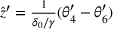
Converting capability to capacity is deterministic, with percentage yield
$δ \in [0, 1]$
. (In Section 4, we extend our analysis to the case when the conversion yield rate δ is uncertain.)
(3)
Ordering inventory and exercising reserved capacity are instantaneous, and therefore meet the demand within the same period.³
(4)
Inventory can be ordered at the beginning of either period, and any inventory left over at the end of period 1 can be carried over to period 2.
(5)
However, shortages occurred at the end of period 1 cannot be carried over to period 2.⁴
(6)
Capacity must be reserved with a supplier for either period separately—reserved capacity cannot be carried over from period 1 to period 2.⁵

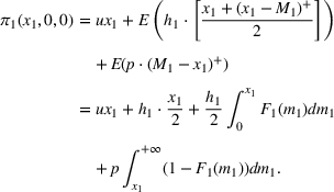
Deploying inventory, capacity, and capability

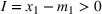
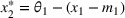
We now describe our two‐period model. At the beginning of period 1, the government decides on the level of (1) stockpile inventory x ₁, (2) backup capacity y ₁, and (3) standby capability z. As a standard modeling assumption for discrete‐time models, the uncertain demand is realized at the end of period 1; that is, m ₁ (Zipkin, 2000). We assume that the demand
$M_{i}$
in period
$i, i = 1, 2$
, follows a general cumulative probability distribution
$F_{i} (\cdot)$
with a density function
$f_{i} (\cdot)$
. Table 1 summarizes our notation.

TABLE 1
Quantities and notation for the two periods

Period 1 Period 2

Stochastic demand $M_{1} \sim F_{1}$
$M_{2} \sim F_{2}$

Realized demand m ₁ m ₂

Inventory ordered x ₁ x ₂

Capability developed z Not applicable, due to time delay

Capacity deployed y ₁
$y_{2} + δ z$
, where
$δ z$
is converted from capability

Leftover inventory
$I = {[x_{1} + y_{1} - m_{1}]}^{+}$

${[I + x_{2} + y_{2} + δ z - m_{2}]}^{+}$

Quantity available
$x_{1} + y_{1}$

$I + x_{2} + y_{2} + δ z$

Shortfall
${[m_{1} - x_{1} - y_{1}]}^{+}$

${[m_{2} - I - x_{2} - y_{2} - δ z]}^{+}$

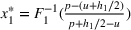
Period 1. Upon observing the realized demand m ₁, the public health authority or relief agency can deploy inventory x ₁ and reserved capacity y ₁ in turn.⁶ Using inventory alone is sufficient if the realized demand m ₁ satisfies
$m_{1} \leq x_{1}$
. However, if
$m_{1} \in (x_{1}, x_{1} + y_{1})$
, then backup capacity y ₁ will have to be used. So, the actual usage of these two resources in period 1 is
$(x_{1}, \min {m_{1} - x_{1}, y_{1}})$
. Finally, if
$m_{1} > (x_{1} + y_{1})$
, then there will be a shortfall of
${[m_{1} - (x_{1} + y_{1})]}^{+}$
in period 1.

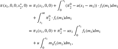
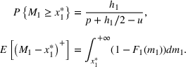
Period 2. At the beginning of period 2, the uncertain demand M ₂ is realized as m ₂ and there is inventory left over from period 1,
$I = {(x_{1} - M_{1})}^{+}$
. There is also manufacturing capacity available from converting capability,
$δ z$
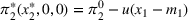
. The government decides on the level of (1) the inventory x ₂ and (2) the backup capacity y ₂. The government first uses inventory
$(I + x_{2})$
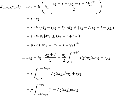
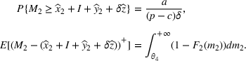
to satisfy the realized demand m ₂. Because the unit cost for using the converted capacity (from capability) is higher than the unit cost for exercising the reserved capacity (as explained in Subsection 2.3), the government will use the reserved capacity y ₂ as the second line of defense, and then use the converted capacity
$δ z$
as the third line of defense to meet the realized demand m ₂ in period 2. If m ₂ exceeds all the available resources
$(I + x_{2} + y_{2} + δ z)$
, then there will be a shortfall of
${[m_{2} - (I + x_{2} + y_{2} + δ z)]}^{+}$
in period 2.

Cost components: Inventory, capacity, and capability

The cost structure associated with inventory, capacity, and capability is as follows. (1)
Stockpile inventory x_i with cost (u, h_i ) in period i = 1, 2. Here, u is the unit cost, and
$h_{i}$
to denote the unit inventory holding cost in period i. We assume that the effective unit holding cost
$h_{i}$
satisfies
$h_{1} \leq h_{2}$
to capture the obsolescence cost of inventory (especially when the inventory has little value at the end of period 2 as in our two‐period model).⁷
(2)
Backup capacity y_i via a capacity reservation contract (r, s) in period i, i = 1, 2. Consider the case when the government develops a capacity reservation contract (cf. Brown & Lee, 2003) with a domestic or regional supplier in period i to establish a backup capacity
$y_{i}$
in period i as follows. First, the government can reserve capacity
$y_{i}$
in advance by paying the supplier r per unit to “reserve” capacity to produce one unit of the product in period i (when necessary). The reservation cost per unit r is paid upfront and is nonrefundable.⁸ The government can “exercise” the capacity reservation contract by paying the supplier an additional s per unit to produce anywhere from 0 to the maximum of
$y_{i}$
units if the need arises.
(3)
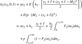
Standby capability z via capability development and deployment with cost (a, c). The government invests a to develop each unit of capability z in period 1 for conversion to production capacity for use in period 2. This capability z can be converted to
$δ z$
units of manufacturing capacity, which has a unit production cost c associated with this converted capacity. We assume
$c > s$
so that it is more economical to exercise the reserved capacity first before using the converted capacity for production as explained earlier. In addition to the costs associated with inventory, capacity, and capability, we impose a penalty p for each unit of shortfall that captures the health‐related cost inflicted on people.⁹

Performance measures

Thus, there are five decisions to be made by the government:
$(x_{1}, y_{1}, z; x_{2}, y_{2})$
for a system that integrates inventory, capacity, and capability over two time periods. Our goal is to determine the optimal decisions that minimize the total expected relevant cost
$π (x_{1}, y_{1}, z; x_{2}, y_{2})$
incurred over the two time periods. The shortfall probability and the expected shortfall are also relevant system performance measures.

ANALYSIS: INVENTORY‐, CAPACITY‐, AND CAPABILITY‐BASED SYSTEMS

We now present our analysis associated with the three nested systems in turn. We begin our analysis of a two‐period system that relies only on stockpiled inventory, so that
$y_{1} = y_{2} = z = 0$
. Next, we examine the system that entails inventory and capacity (i.e., when
$z = 0$
), followed by the analysis of the third system that uses all three resources: inventory, capacity, and capability. We compare the total relevant cost across all three systems and identify the conditions under which the government should develop a system that integrates all three resources.

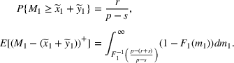
Inventory‐based system

Consider the inventory‐based system in Figure 1. Recall that, in period 1, the government decides on the stockpile inventory x ₁, which is the only resource available to satisfy period 1's uncertain demand M ₁. If the realized period‐1 demand m ₁ is smaller than x ₁, then the left‐over inventory
$I = x_{1} - m_{1} > 0$
can be carried over to period 2; otherwise,
$I = 0$
. In period 2, the government decides on the stockpile inventory x ₂ so that x ₂ together with the left‐over inventory of the previous period
$I = {(x_{1} - m_{1})}^{+}$
can be used to satisfy period 2's uncertain demand M ₂.

FIGURE 1
Inventory‐based system
$(x_{1}, 0, 0; x_{2}, 0)$
with realized demand m ₁ and m ₂ of periods 1 and 2 to be met solely from inventory

We assume that
$h_{1} \leq h_{2}$
to capture the obsolescence cost of inventory. Recall that the unit cost is u, the holding cost
$h_{i}$
, and the penalty cost p for each unit of unmet demand in either period i; the penalty cost is high by assumptions so that
$p > u + h_{2} / 2$
. We now use backward induction to determine the optimal values
$(x_{1}^{}, 0, 0; x_{2}^{}, 0)$
that minimize the expected total cost
$π (x_{1}, 0, 0; x_{2}, 0)$
.¹⁰

In period 2, the leftover inventory from period 1
$I = {[x_{1} - m_{1}]}^{+}$
is known, and the total expected relevant cost in period 2 for ordering x ₂ units of inventory is:
$\begin{matrix} π_{2} (x_{2}, 0; I) & = & u x_{2} + E (h_{2} \cdot [\frac{x_{2} + I + {(x_{2} + I - M_{2})}^{+}}{2}]) \\ + E (p \cdot {[M_{2} - (x_{2} + I)]}^{+}) \\ = & u x_{2} + h_{2} \cdot \frac{x_{2} + I}{2} + \frac{h_{2}}{2} \int_{0}^{x_{2} + I} F_{2} (m_{2}) d m_{2} \\ + p \int_{x_{2} + I}^{+ \infty} (1 - F_{2} (m_{2})) d m_{2} . \end{matrix}$
1
Notice that the initial and ending inventory are
$x_{2} + I$
and
${(x_{2} + I - M_{2})}^{+}$
; respectively. Hence, the average inventory cost throughout the period is
$h_{2} \cdot [\frac{x_{2} + I + {(x_{2} + I - M_{2})}^{+}}{2}]$
.¹¹ Observe that the relevant cost
$π_{2} (x_{2}, 0, 0)$
given in (1) possesses the same structure as the classical newsvendor problem. Hence, we use the following lemma to characterize the optimal
$x_{2}^{}$
. For ease of exposition, we denote the threshold
$θ_{1} \equiv F_{2}^{- 1} (\frac{p - (u + h_{2} / 2)}{p + h_{2} / 2})$
, where
$θ_{1} > 0$
because of our assumption that
$p > (u + h_{2} / 2)$
.¹² Lemma 1
Given the left‐over inventory from period 1
$I = {(x_{1} - m_{1})}^{+}$
, the optimal stockpile inventory in period 2 is
$x_{2}^{} = θ_{1} - I$
, where
$θ_{1} = F_{2}^{- 1} (\frac{p - (u + h_{2} / 2)}{p + h_{2} / 2})$
. Specifically, (1)
when
$m_{1} \geq x_{1}$
so that
$I = 0$
,
$x_{2}^{} = θ_{1}$
and
$π_{2}^{} (x_{2}^{}, 0, 0) = (u + \frac{h_{2}}{2}) θ_{1} + \frac{h_{2}}{2} \int_{0}^{θ_{1}} F_{2} (m_{2}) d m_{2} + p \int_{θ_{1}}^{\infty} (1 - F_{2} (m_{2})) d m_{2} \equiv π_{2}^{0}$
;
(2)
when
$m_{1} < x_{1}$
so that
$I = x_{1} - m_{1} > 0$
,
$x_{2}^{} = θ_{1} - (x_{1} - m_{1})$
and
$π_{2}^{} (x_{2}^{}, 0, 0) = π_{2}^{0} - u (x_{1} - m_{1})$
.¹³

Observe from statement 1 in Lemma 1 that, when
$m_{1} \geq x_{1}$
so that
$I = 0$
, both the optimal stockpile inventory
$x_{2}^{}$
and the optimal cost
$π_{2}^{0}$
for period 2 depend on θ₁, which is independent of x ₁ and m ₁. Armed with Lemma 1, we proceed to solve the problem at the beginning of period 1.

The total expected relevant cost* for ordering x ₁ units of inventory at the beginning of period 1 is:
$\begin{matrix} π_{1} (x_{1}, 0, 0) & = & u x_{1} + E (h_{1} \cdot [\frac{x_{1} + {(x_{1} - M_{1})}^{+}}{2}]) \\ + E (p \cdot {(M_{1} - x_{1})}^{+}) \\ = & u x_{1} + h_{1} \cdot \frac{x_{1}}{2} + \frac{h_{1}}{2} \int_{0}^{x_{1}} F_{1} (m_{1}) d m_{1} \\ + p \int_{x_{1}}^{+ \infty} (1 - F_{1} (m_{1})) d m_{1} . \end{matrix}$
2
Combining the cost
$π_{1} (x_{1}, 0, 0)$
incurred in period 1 and
$π_{2}^{} (x_{2}^{}, 0, 0)$
incurred in period 2 as stated in Lemma 1, the total expected cost for the inventory‐based system is:
$\begin{matrix} π (x_{1}, 0, 0; x_{2}^{}, 0) & = & π_{1} (x_{1}, 0, 0) + \int_{0}^{x_{1}} (π_{2}^{0} - u (x_{1} - m_{1})) \cdot f_{1} (m_{1}) d m_{1} \\ + \int_{x_{1}}^{\infty} π_{2}^{0} \cdot f_{1} (m_{1}) d m_{1} \\ = & π_{1} (x_{1}, 0, 0) + π_{2}^{0} - u x_{1} \int_{0}^{x_{1}} f_{1} (m_{1}) d m_{1} \\ + u \int_{0}^{x_{1}} m_{1} f_{1} (m_{1}) d m_{1}, \end{matrix}$
3
where
$π_{2}^{0}$
is independent of x ₁. By minimizing
$π (x_{1}, 0, 0; x_{2}^{}, 0)$
, we obtain the following. Proposition 1 Inventory‐based system

	Period 1	Period 2
Stochastic demand	$M_{1} \sim F_{1}$	$M_{2} \sim F_{2}$
Realized demand	m ₁	m ₂
Inventory ordered	x ₁	x ₂
Capability developed	z	Not applicable, due to time delay
Capacity deployed	y ₁	$y_{2} + δ z$ , where $δ z$ is converted from capability
Leftover inventory	$I = {[x_{1} + y_{1} - m_{1}]}^{+}$	${[I + x_{2} + y_{2} + δ z - m_{2}]}^{+}$
Quantity available	$x_{1} + y_{1}$	$I + x_{2} + y_{2} + δ z$
Shortfall	${[m_{1} - x_{1} - y_{1}]}^{+}$	${[m_{2} - I - x_{2} - y_{2} - δ z]}^{+}$

When the holding costs

h_{2} \geq h_{1}

and the penalty cost

p > u + h_{2} / 2

, the optimal inventory‐based system

(x_{1}^{*}, 0, 0; x_{2}^{*}, 0)

satisfies the following.

(1)
In period 1, the optimal stockpile inventory
$x_{1}^{} = F_{1}^{- 1} (\frac{p - (u + h_{1} / 2)}{p + h_{1} / 2 - u})$
so that the shortfall probability and the expected shortfall of period 1 are:
$\begin{matrix} P \{M_{1} \geq x_{1}^{}\} & = & \frac{h_{1}}{p + h_{1} / 2 - u}, \\ E [{(M_{1} - x_{1}^{})}^{+}] & = & \int_{x_{1}^{}}^{+ \infty} (1 - F_{1} (m_{1})) d m_{1} . \end{matrix}$
4

(2)
In period 2, the optimal stockpile inventory
$x_{2}^{} = F_{2}^{- 1} (\frac{p - (u + h_{2} / 2)}{p + h_{2} / 2}) - {(x_{1}^{} - m_{1})}^{+}$
so that the shortfall probability and the expected shortfall of period 2 are:
$\begin{matrix} P {M_{2} \geq [x_{2}^{} + {(x_{1}^{} - m_{1})}^{+}]} = \frac{u + h_{2}}{p + h_{2} / 2}, \\ E [{(M_{2} - x_{2}^{} - {(x_{1}^{} - m_{1})}^{+})}^{+}] = \int_{x_{2}^{} + {(x_{1}^{} - m_{1})}^{+}}^{+ \infty} (1 - F_{2} (m_{2})) d m_{2} . \end{matrix}$
5

From Proposition 1 and our assumption that the penalty cost is high so that
$p > u + h_{2} / 2 \geq u + h_{1} / 2$
, we conclude that
$x_{1}^{} > 0$
. Also, when the condition
$p > u + h_{2} / 2$
holds, it is easy to check that the optimal inventory of both periods
$x_{1}^{}$
and
$x_{2}^{}$
increases as the penalty cost p for each unit unmet demand. Consequently, both the shortfall probability and the expected shortfall of both periods decrease with an increasing penalty cost p.

By comparing periods 1 and 2, we obtain the following corollary. Corollary 1
In the optimal inventory‐based system, the shortfall probability of period 1 is lower than that of period 2, that is,
$P {M_{1} \geq x_{1}^{}} < P {M_{2} \geq [x_{2}^{} + {(x_{1}^{} - m_{1})}^{+}]}$
. Moreover, if the demand distribution is the same in both periods (i.e.,
$F_{1} (\cdot) = F_{2} (\cdot)$
), then the optimal stockpile inventory
$x_{1}^{} > x_{2}^{}$
and the expected shortfall
$E [{(M_{1} - x_{1}^{})}^{+}] < E [{(M_{2} - x_{2}^{} - {(x_{1}^{} - m_{1})}^{+})}^{+}]$
.

Corollary 1 suggests that it is optimal to keep the shortage probability for period 1 lower than that for period 2, regardless of the underlying demand distribution
$F_{i} (\cdot)$
in either period i. Also, when the demand distribution for both periods is the same, Corollary 1 implies that it is optimal to set a higher inventory level in period 1 so that the expected shortfall of period 1 is less than that of period 2. These two results are due to the fact that, in our two‐period model, left‐over inventory from period 1 can be carried over to period 2. As such, it is less risky to order more in period 1, resulting in a lower shortfall probability in period 1.

Capacity‐based system

Consider the capacity‐based system that involves inventory
$x_{i}$
and backup capacity
$y_{i}$
in period i (Figure 2).

FIGURE 2
Capacity‐based system
$(x_{1}, y_{1}, 0; x_{2}, y_{2})$
with realized demand m ₁ and m ₂ of periods 1 and 2 to be met first from inventory and only after inventory is exhausted from backup capacity.

In period 1, the government determines the stockpile inventory x ₁ and the backup capacity y ₁. Here, x ₁ is the first deployed to satisfy the realized demand m ₁, and the backup capacity y ₁ is called upon only after exhausting x ₁. Subsequently, in period 2, the government determines the stockpile inventory x ₂ and the backup capacity y ₂ after observing the left‐over inventory from period 1
$I = {(x_{1} - m_{1})}^{+}$
. The government will use the left‐over inventory from period 1
$I = {(x_{1} - m_{1})}^{+}$
and the newly acquired inventory x ₂ to satisfy the realized demand m ₂. The reserved capacity y ₂ will be exercised after exhausting
$I + x_{2}$
. As before, we use backward induction to determine the optimal values of
$({\tilde{x}}_{1}, {\tilde{y}}_{1}, 0; {\tilde{x}}_{2}, {\tilde{y}}_{2})$
that minimize the total expected cost
$π (x_{1}, y_{1}, 0; x_{2}, y_{2})$
.

Period 2. In period 2, given the left‐over inventory of period 1 as
$I = {(x_{1} - m_{1})}^{+}$
, the total expected relevant cost of period 2 for the capacity‐based system is:
$\begin{matrix} π_{2} (x_{2}, y_{2}; I) & = & u x_{2} + E (h_{2} [\frac{x_{2} + I + {(x_{2} + I - M_{2})}^{+}}{2}]) \\ + r \cdot y_{2} \\ + s \cdot E (M_{2} - (x_{2} + I) | M_{2} \in [x_{2} + I, x_{2} + I + y_{2}]) \\ + s \cdot E (y_{2} | M_{2} \geq (x_{2} + I + y_{2})) \\ + p \cdot E ({[M_{2} - (x_{2} + I + y_{2})]}^{+}) \\ = & u x_{2} + h_{2} \cdot \frac{x_{2} + I}{2} + \frac{h_{2}}{2} \int_{0}^{x_{2} + I} F_{2} (m_{2}) d m_{2} + r y_{2} \\ - s \int_{x_{2} + I}^{x_{2} + I + y_{2}} F_{2} (m_{2}) d m_{2} + s y_{2} \\ + p \int_{x_{2} + I + y_{2}}^{+ \infty} (1 - F_{2} (m_{2})) d m_{2} . \end{matrix}$
6

The first two terms in (6) are the ordering and holding costs as in (1). The third term
$r \cdot y_{2}$
corresponds to the upfront backup capacity reservation cost for period 2. This backup capacity is called upon only when demand
$M_{2} > x_{2} + I$
. Specifically, as shown in Figure 2, when
$M_{2} \in [x_{2} + I, x_{2} + I + y_{2}]$
, the fourth term represents the cost for exercising
$(M_{2} - (x_{2} + I))$
units of the backup capacity to satisfy the remaining demand
$(M_{2} - (x_{2} + I))$
at s per unit. The fifth term
$s \cdot y_{2}$
captures the cost of using all of the backup capacity when
$M_{2} \geq x_{2} + I + y_{2}$
, and the last term corresponds to the penalty cost of the shortfall
${[M_{2} - (x_{2} + I + y_{2})]}^{+}$
. We obtain the optimal
$({\tilde{x}}_{2}, {\tilde{y}}_{2})$
by minimizing
$π_{2} (x_{2}, y_{2}, 0)$
as given in the following lemma. Lemma 2
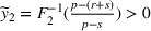
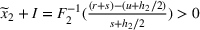
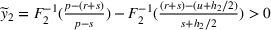
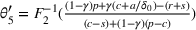
In the capacity‐based system, given any inventory left over from period 1
$I = {(x_{1} - m_{1})}^{+}$
, the optimal
$({\tilde{x}}_{2}, {\tilde{y}}_{2})$
in period 2 has the following properties: (1)
If
$r \leq u + h_{2} / 2 - s$
, then
${\tilde{x}}_{2} + I = 0$
and
${\tilde{y}}_{2} = F_{2}^{- 1} (\frac{p - (r + s)}{p - s}) > 0$
.
(2)
If
$r \in (u + h_{2} / 2 - s, \frac{(p - s) (h_{2} + u)}{h_{2} / 2 + p})$
, then
${\tilde{x}}_{2} + I = F_{2}^{- 1} (\frac{(r + s) - (u + h_{2} / 2)}{s + h_{2} / 2}) > 0$
and
${\tilde{y}}_{2} = F_{2}^{- 1} (\frac{p - (r + s)}{p - s}) - F_{2}^{- 1} (\frac{(r + s) - (u + h_{2} / 2)}{s + h_{2} / 2}) > 0$
.
(3)
If
$r \geq \frac{(p - s) (h_{2} + u)}{h_{2} / 2 + p}$
, then
${\tilde{x}}_{2} + I = F_{2}^{- 1} (\frac{p - (u + h_{2} / 2)}{p + h_{2} / 2}) > 0$
and
${\tilde{y}}_{2} = 0$
.

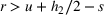
Lemma 2 captures the trade‐off between inventory and capacity in period 2. The first statement indicates that inventory is not needed when the capacity reservation and exercise cost
$r + s \leq u + \frac{h_{2}}{2}$
. This is because when the unit reservation cost and the exercise cost are lower than the unit cost and the average holding cost, it is more economical to reserve capacity instead of keeping inventory. However, in practice, it is more likely to have
$r + s > u + \frac{h_{2}}{2}$
so that inventory is needed. Specifically, the second statement implies that it is optimal to leverage both the stockpile inventory and backup capacity only when the reservation cost r is moderate (i.e.,
$r \in (u + h_{2} / 2 - s, \frac{(p - s) (h_{2} + u)}{h_{2} / 2 + p})$
). Finally, the third statement of the lemma implies that capacity is not needed when the reservation cost r is sufficiently high, and in this case, the optimal
${\tilde{x}}_{2}$
under the capacity‐based system is the same as
$x_{2}^{}$
under the inventory‐based system.

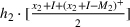
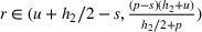
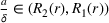
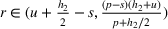
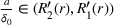
Denote the thresholds
$θ_{1} = F_{2}^{- 1} (\frac{p - (u + h_{2} / 2)}{p + h_{2} / 2})$
,
$θ_{2} = F_{2}^{- 1} (\frac{(r + s) - (u + h_{2} / 2)}{s + h_{2} / 2})$
, and
$θ_{3} = F_{2}^{- 1} (\frac{p - (r + s)}{p - s})$
. By substituting the optimal
$({\tilde{x}}_{2}, {\tilde{y}}_{2})$
from Lemma 2 into (6), we can retrieve the corresponding optimal cost
$π_{2} ({\tilde{x}}_{2}, {\tilde{y}}_{2}; I)$
in period 2 as:
$\begin{matrix} π_{2} ({\tilde{x}}_{2}, {\tilde{y}}_{2} | I = 0) \equiv {\tilde{π}}_{2}^{0}, where \end{matrix}$
7

$\begin{matrix} {\tilde{π}}_{2}^{0} & = \{\begin{matrix} (r + s) \cdot θ_{3} - s \int_{0}^{θ_{3}} F_{2} (m_{2}) d m_{2} + p \int_{θ_{3}}^{+ \infty} (1 - F_{2} (m_{2})) d m_{2} & r \leq u + h_{2} / 2 - s; \\ (u + h_{2} / 2) θ_{2} + \frac{h_{2}}{2} \int_{0}^{θ_{2}} F_{2} (m_{2}) d m_{2} + (r + s) (θ_{3} - θ_{2}) \\ - s \int_{θ_{2}}^{θ_{3}} F_{2} (m_{2}) d m_{2} + p \int_{θ_{3}}^{+ \infty} (1 - F_{2} (m_{2})) d m_{2} & r \in (u + h_{2} / 2 - s, \frac{(p - s) (h_{2} + u)}{h_{2} / 2 + p}); \\ (u + h_{2} / 2) θ_{1} + \frac{h_{2}}{2} \int_{0}^{θ_{1}} F_{2} (m_{2}) d m_{2} + p \int_{θ_{1}}^{+ \infty} (1 - F_{2} (m_{2})) d m_{2} \equiv π_{2}^{0} & r \geq \frac{(p - s) (h_{2} + u)}{h_{2} / 2 + p}; \end{matrix} \\ π_{2} ({\tilde{x}}_{2}, {\tilde{y}}_{2} | I = x_{1} - m_{1} > 0) = {\tilde{π}}_{2}^{0} - u (x_{1} - m_{1}) . \end{matrix}$
8
From (7) and (8), we conclude that when
$I = 0$
, the optimal cost of period 2
${\tilde{π}}_{2}^{0}$
is independent of the government decision
$(x_{1}, y_{1})$
for period 1 and the realized demand m ₁ of period 1. Also, when the reservation cost r is sufficiently high so that the optimal
${\tilde{y}}_{2} = 0$
, then the optimal cost of the capacity‐based system would be the same as that of the inventory‐based system. Armed with the optimal cost in period 2 as given in (7) and (8), we proceed to analyze period 1's problem.

Period 1. The expected relevant cost incurred in period 1 can be expressed as:
$\begin{matrix} π_{1} (x_{1}, y_{1}, 0) & = & u x_{1} + E (h_{1} [\frac{x_{1} + {(x_{1} - M_{1})}^{+}}{2}]) + r \cdot y_{1} \\ + s \cdot E (M_{1} - x_{1} | M_{1} \in [x_{1}, x_{1} + y_{1}]) \\ + s \cdot E (y_{1} | M_{1} \geq (x_{1} + y_{1})) + p \cdot E ({[M_{1} - (x_{1} + y_{1})]}^{+}) \\ = & u x_{1} + h_{1} \cdot \frac{x_{1}}{2} + \frac{h_{1}}{2} \int_{0}^{x_{1}} F_{1} (m_{1}) d m_{1} + r y_{1} \\ - s \int_{x_{1}}^{x_{1} + y_{1}} F_{1} (m_{1}) d m_{1} + s y_{1} \\ + p \int_{x_{1} + y_{1}}^{+ \infty} (1 - F_{1} (m_{1})) d m_{1} . \end{matrix}$
9
Combining the above cost and the optimal expected cost for this system in period 2
$π_{2} ({\tilde{x}}_{2}, {\tilde{y}}_{2}; I)$
, the total expected cost is:
$\begin{matrix} π (x_{1}, y_{1}, 0; {\tilde{x}}_{2}, {\tilde{y}}_{2}) & = & π_{1} (x_{1}, y_{1}, 0) + \int_{0}^{x_{1}} ({\tilde{π}}_{2}^{0} - u (x_{1} - m_{1})) \cdot f_{1} (m_{1}) d m_{1} \\ + \int_{x_{1}}^{\infty} {\tilde{π}}_{2}^{0} \cdot f_{1} (m_{1}) d m_{1} \\ = & π_{1} (x_{1}, y_{1}, 0) + {\tilde{π}}_{2}^{0} - u x_{1} \int_{0}^{x_{1}} f_{1} (m_{1}) d m_{1} \\ + u \int_{0}^{x_{1}} m_{1} f_{1} (m_{1}) d m_{1}, \end{matrix}$
10

where
${\tilde{π}}_{2}^{0}$
is independent of x ₁. By minimizing the total expected cost
$π (x_{1}, y_{1}, 0; {\tilde{x}}_{2}, {\tilde{y}}_{2}, 0)$
, we obtain the optimal government decision in the following proposition. Proposition 2 Capacity‐based system

Under the capacity‐based system, the optimal

({\tilde{x}}_{1}, {\tilde{y}}_{1}, 0; {\tilde{x}}_{2}, {\tilde{y}}_{2})

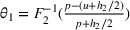
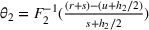
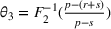
satisfies the following:

(1)
In period 1, the optimal stockpile inventory
${\tilde{x}}_{1}$
and the backup capacity
${\tilde{y}}_{1}$
are: (a)
If
$r \leq u + h_{1} / 2 - s$
, then
${\tilde{x}}_{1} = 0$
,
${\tilde{y}}_{1} = F_{1}^{- 1} (\frac{p - (r + s)}{p - s}) > 0$
.
(b)
If
$r \in (u + h_{1} / 2 - s, \frac{h_{1} (p - s)}{p - u + h_{1} / 2})$
, then
${\tilde{x}}_{1} = F_{1}^{- 1} (\frac{r + s - (u + h_{1} / 2)}{h_{1} / 2 + s - u}) > 0$
and
${\tilde{y}}_{1} = F_{1}^{- 1} (\frac{p - (r + s)}{p - s}) - F_{1}^{- 1} (\frac{r + s - (u + h_{1} / 2)}{h_{1} / 2 + s - u}) > 0$
.
(c)
If
$r \geq \frac{h_{1} (p - s)}{p - u + h_{1} / 2}$
, then
${\tilde{x}}_{1} = F_{1}^{- 1} (\frac{p - (u + h_{1} / 2)}{p - u + h_{1} / 2}) > 0$
and
${\tilde{y}}_{1} = 0$
.
Also, when
$r < \frac{h_{1} (p - s)}{p - u + h_{1} / 2}$
, the shortfall probability and the expected shortfall of period 1 under capacity‐based system are
$\begin{matrix} P {M_{1} \geq {\tilde{x}}_{1} + {\tilde{y}}_{1}} & = & \frac{r}{p - s}, \\ E [{(M_{1} - ({\tilde{x}}_{1} + {\tilde{y}}_{1}))}^{+}] & = & \int_{F_{1}^{- 1} (\frac{p - (r + s)}{p - s})}^{\infty} (1 - F_{1} (m_{1})) d m_{1} . \end{matrix}$
11
However, when
$r \geq \frac{h_{1} (p - s)}{p - u + h_{1} / 2}$
, the shortfall probability and the expected shortfall of period 1 under capacity‐based system are the same as the inventory‐based system, which are given by (4).
(2)
In period 2, the optimal
$({\tilde{x}}_{2}, {\tilde{y}}_{2})$
is as given by Lemma 2. Also, when
$r < \frac{(p - s) (h_{2} + u)}{h_{2} / 2 + p}$
, the shortfall probability and the expected shortfall of period 2 under capacity‐based system are
$\begin{matrix} P {M_{2} \geq {\tilde{x}}_{2} + I + {\tilde{y}}_{2}} & = & \frac{r}{p - s}, \\ E [{(M_{2} - ({\tilde{x}}_{2} + I + {\tilde{y}}_{2}))}^{+}] & = & \int_{F_{2}^{- 1} (\frac{p - (r + s)}{p - s})}^{\infty} (1 - F_{2} (m_{2})) d m_{2} . \end{matrix}$
12
However, when
$r \geq \frac{(p - s) (h_{2} + u)}{h_{2} / 2 + p}$
, the shortfall probability and the expected shortfall of period 2 under capacity‐based system are the same as the inventory‐based system, which are given by (5).

From Proposition 2, we observe that the optimal decision
$({\tilde{x}}_{1}, {\tilde{y}}_{1})$
in period 1 has a structure similar to
$({\tilde{x}}_{2}, {\tilde{y}}_{2})$
of period 2 given by Lemma 2. So, it is optimal to leverage both the stockpile inventory and backup capacity only when the reservation cost r is moderate. Otherwise, when the reservation cost r is too high capacity is not needed and when it is too low, inventory is not needed. In particular, statement 1(c) reveals that when
$r \geq \frac{h_{1} (p - s)}{p - u + h_{1} / 2}$
, the optimal
${\tilde{x}}_{1}$
is the same as
$x_{1}^{}$
for the inventory‐based system as stated in Proposition 1. When the reservation cost r is moderate (i.e.,
$r \in (u + h_{2} / 2 - s, \frac{h_{1} (p - s)}{p - u + h_{1} / 2})$
) the government should leverage both inventory and capacity in periods 1 and 2. Then, we can compare the optimal decisions of the two periods to obtain the following. Corollary 2
Suppose the reservation cost
$r \in (u + h_{2} / 2 - s, \frac{h_{1} (p - s)}{p - u + h_{1} / 2})$
so that the government should leverage both inventory and capacity under the capacity‐based system in both periods. (1)*
Then the shortfall probability of period 1 is the same as period 2, that is,
$P {M_{1} \geq {\tilde{x}}_{1} + {\tilde{y}}_{1}} = P {M_{2} \geq {\tilde{x}}_{2} + {(x_{1} - m_{1})}^{+} + {\tilde{y}}_{2}} = \frac{r}{p - s}$
.
(2)
Also, if the demand distribution is the same in both periods (i.e.,
$F_{1} (\cdot) = F_{2} (\cdot)$
), then the optimal stockpile inventory
${\tilde{x}}_{1} > {\tilde{x}}_{2}$
and the backup capacity
${\tilde{y}}_{1} < {\tilde{y}}_{2}$
. Also, the expected shortfalls of the two periods are the same, that is,
$E [{(M_{1} - ({\tilde{x}}_{1} + {\tilde{y}}_{1}))}^{+}] = E [{(M_{2} - ({\tilde{x}}_{2} + {({\tilde{x}}_{1} - m_{1})}^{+} + {\tilde{y}}_{2}))}^{+}]$
.

When the reservation cost r is moderate, Corollary 2 for the capacity‐based system generates results different from those for the inventory‐based system. Under the capacity‐based system, the government should ensure the shortfall probability of the two periods at the same level regardless of the demand distribution. Also, when the demand distribution for both periods are the same (i.e.,
$F_{1} (\cdot) = F_{2} (\cdot)$
), it is optimal for the government to set a higher stockpile inventory level in period 1 and a higher backup capacity level in period 2. This is because the inventory in period 1 can be carried over to period 2, but not the reserved capacity. Also, when the demand distribution is the same, the shortfall probability and the expected shortfalls of the two periods are equal.

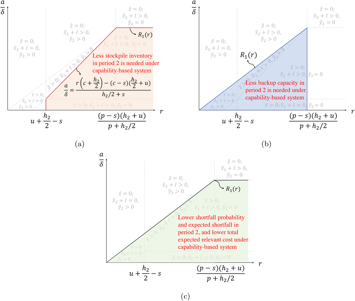
Comparing capacity‐based versus inventory‐based systems

We now compare the performance between the optimal inventory‐based system and capacity‐based system as stated in Propositions 1 and 2 as follows. Corollary 3
Comparing with the optimal inventory‐based system
$(x_{1}^{}, 0, 0; x_{2}^{}, 0)$
, the optimal capacity‐based system
$({\tilde{x}}_{1}, {\tilde{y}}_{1}, 0; {\tilde{x}}_{2}, {\tilde{y}}_{2})$
has the following properties: (1)
Stockpile inventory. In period 1, less inventory is needed under the capacity‐based system (i.e.,
${\tilde{x}}_{1} < x_{1}^{}$
) if and only if
$r < \frac{h_{1} (p - s)}{p - u + h_{1} / 2}$
. In period 2, given the same left‐over inventory I, less inventory is needed under the capacity‐based system (i.e.,
${\tilde{x}}_{2} < x_{2}^{}$
) if and only if
$r < \frac{(p - s) (h_{2} + u)}{h_{2} / 2 + p}$
.
(2)
Shortfall probability and expected shortfall. In period 1, the shortfall probability and the expected shortfall are both strictly lower under the capacity‐based system (i.e.,
$P {M_{1} \geq {\tilde{x}}_{1} + {\tilde{y}}_{1}} < P {M_{1} \geq x_{1}^{}}$
and
$E [{(M_{1} - ({\tilde{x}}_{1} + {\tilde{y}}_{1}))}^{+}] < E [{(M_{1} - x_{1}^{})}^{+}]$
) if and only if the reservation cost
$r < \frac{h_{1} (p - s)}{p - u + h_{1} / 2}$
. In period 2, the shortfall probability and the expected shortfall are both strictly lower under the capacity‐based system (i.e.,
$P {M_{2} \geq {\tilde{x}}_{2} + I + {\tilde{y}}_{2}} < P {M_{2} \geq x_{2}^{} + I}$
and
$E [{(M_{2} - ({\tilde{x}}_{2} + I + {\tilde{y}}_{2}))}^{+}] < E [{(M_{2} - (x_{2}^{} + I))}^{+}]$
) if and only if the reservation cost
$r < \frac{(p - s) (h_{2} + u)}{h_{2} / 2 + p}$
.
(3)
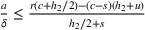
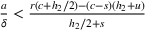
Expected relevant cost. The capacity‐based system incurs a strictly lower relevant cost than the inventory‐based system (i.e.,
$π ({\tilde{x}}_{1}, {\tilde{y}}_{1}, 0; {\tilde{x}}_{2}, {\tilde{y}}_{2}) < π (x_{1}^{}, 0, 0; x_{2}^{}, 0)$
) when
$r < \frac{(p - s) (h_{2} + u)}{h_{2} / 2 + p}$
.

Corollary 3 has the following implications. The extra option of backup capacity can lower the relevant cost when
$r < \frac{(p - s) (h_{2} + u)}{h_{2} / 2 + p}$
as stated in statement 3 of Corollary 3. Still, statements 1 and 2 offer two interesting insights. First, it is not necessarily true that the capacity‐based system will always reduce the inventory level and outperform the inventory‐based system. Specifically, statement 1 states that the capacity‐based system can result in lower inventory only when the reservation cost r is below certain thresholds in both periods. Second, it is not necessarily true that the capacity‐based system will always reduce the shortfall probability and the expected shortfalls. Specifically, statement 2 shows that the capacity‐based system can reduce the shortfall probability and the expected shortfalls only when the reservation cost r is below certain thresholds. Hence, Corollary 3 implies that the capacity‐based system dominates the inventory‐based system in terms of stockpile inventory and shortfall‐related performances only when the cost structure of the backup capacity
$(r, s)$
is sufficiently low.

Capability‐based system

Consider the capability‐based system
$(x_{1}, y_{1}, z; x_{2}, y_{2})$
depicted in Figure 3.

FIGURE 3
Capability‐based system
$(x_{1}, y_{1}, z; x_{2}, y_{2})$
with realized demand m ₁ and m ₂ of periods 1 and 2

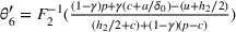
Because capability involves R&D and other technology development activities, we introduce two salient features to distinguish the capability‐based system from the other two systems as explained in Section 3: (1) We assume that capability conversion is a time‐consuming process that takes the entire first period to convert the standby capability into production capacity for use in the second period. (Due to this delay, we consider capability in the first period only.) (2) We assume that the conversion yield from capability to capacity is δ, where
$δ < 1$
, where δ is fixed and deterministic—in Section 5, we extend our analysis to the case when δ is uncertain.

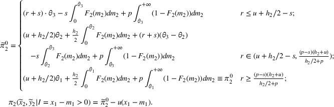
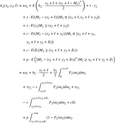
Observe from Figure 3 that the government determines the stockpile inventory x ₁, the backup capacity y ₁, and the standby capability z in period 1. Here, the three‐tiered response follows a sequence similar to what we saw before.

The upfront investment cost for developing the standby capability z in period 1 is
$a \cdot z$
, where a represents the per‐unit fixed development cost. Converting the standby capability z into production capacity
$δ z$
will take the entire period 1, and the unit cost for using the converted capacity is c. In period 2, the government first observes the left‐over inventory from period 1
$I = {(x_{1} - m_{1})}^{+}$
, and then determines the stockpile inventory level x ₂ and the backup capacity level y ₂. Again, the government will first use the left‐over inventory
$I = {(x_{1} - m_{1})}^{+}$
and the newly acquired inventory x ₂, then deploy backup capacity y ₂ as needed. The converted capacity (from period 1)
$δ z$
will be called upon after exhausting
$I + x_{2} + y_{2}$
.

As before, we use backward induction to determine the optimal
$({\hat{x}}_{1}, {\hat{y}}_{1}, z; {\hat{x}}_{1}, {\hat{y}}_{2})$
that minimizes the total expected cost
$π (x_{1}, y_{1}, z; x_{2}, y_{2})$
.

Period 2. In period 2, the leftover inventory from period 1
$I = {(x_{1} - m_{1})}^{+}$
is known. Hence, the total expected relevant cost incurred in period 2 for the capability‐based system is:
$\begin{matrix} π_{2} (x_{2}, y_{2}; I) & = & u x_{2} + E (h_{2} \cdot \frac{x_{2} + I + {(x_{2} + I - M_{2})}^{+}}{2}) + r \cdot y_{2} \\ + s \cdot E ((M_{2} - (x_{2} + I)) | M_{2} \in [x_{2} + I, x_{2} + I + y_{2}]) \\ + s \cdot E (y_{2} | M_{2} \geq (x_{2} + I + y_{2})) \\ + c \cdot E ((M_{2} - (x_{2} + I + y_{2})) | M_{2} \in [x_{2} + I + y_{2}, \\ x_{2} + I + y_{2} + δ z]) \\ + c \cdot E (δ z | M_{2} \geq (x_{2} + I + y_{2} + δ z)) \\ + p \cdot E ({[M_{2} - (x_{2} + I + y_{2} + δ z)]}^{+} | M_{2} \geq x_{2} + I + y_{2} + δ z) \\ = & u x_{2} + h_{2} \cdot \frac{x_{2} + I}{2} + \frac{h_{2}}{2} \int_{0}^{x_{2} + I} F_{2} (m_{2}) d m_{2} \\ + r y_{2} - s \int_{x_{2} + I}^{x_{2} + I + y_{2}} F_{2} (m_{2}) d m_{2} + s y_{2} \\ - c \int_{x_{2} + I + y_{2}}^{x_{2} + I + y_{2} + δ z} F_{2} (m_{2}) d m_{2} + c δ z \\ + p \int_{x_{2} + I + y_{2} + δ z}^{+ \infty} (1 - F_{2} (m_{2})) d m_{2} . \end{matrix}$
13
Observe that the first five terms in (13) capture the various costs associated with the stockpile inventory x ₂ and backup capacity y ₂ as in the capacity‐based system that are given in (7). The remaining terms are attributed to the standby capability z established in period 1. In Figure 3, note that the standby capability can be converted to production capacity
$δ z$
in period 2 and the converted capacity will be deployed for production only when demand
$M_{2} > (x_{2} + I + y_{2})$
(i.e., after both the inventory and backup capacity are exhausted). Specifically, when
$M_{2} \in [x_{2} + I + y_{2}, x_{2} + I + y_{2} + δ z]$
, the first of the remaining terms represents the cost of deploying the “converted capacity” to meet the shortfall
$M_{2} - (x_{2} + I + y_{2})$
for the given yield rate δ. Similarly, when
$M > x_{2} + I + y_{2} + δ z$
, the first term of the last line captures the cost of using all converted capacity
$δ z$
. The last term is the penalty for the shortfall
${[M_{2} - (x_{2} + I + y_{2} + δ z)]}^{+}$
.

By differentiating
$π_{2} (x_{2}, y_{2}; I)$
with respect to x ₂ and y ₂, we can check that both the optimal
$({\hat{x}}_{2}, {\hat{y}}_{2})$
and
${\hat{π}}_{2} ({\hat{x}}_{2}, {\hat{y}}_{2}; I)$
depend on the capability level z established in period 1. Analogous to the inventory‐based and capacity‐based systems, we define the optimal relevant cost of the capability‐based system for the case when
$I = 0$
as
${\hat{π}}_{2}^{0}$
(i.e.,
${\hat{π}}_{2}^{0} \equiv π_{2} ({\hat{x}}_{2}, {\hat{y}}_{2}; I = 0)$
) so that
${\hat{π}}_{2}^{0}$
is independent of x ₁ and m ₁. Also, we can obtain that for the case when
$I = x_{1} - m_{1} > 0$
, the optimal
$π_{2} ({\hat{x}}_{2}, {\hat{y}}_{2}; I = x_{1} - m_{1} > 0) = {\hat{π}}_{2}^{0} - u (x_{1} - m_{1})$
. We next proceed to analyze period 1's problem.

Period 1. The total expected relevant cost of period 1 for the capability‐based system is:
$\begin{matrix} π_{1} (x_{1}, y_{1}, z) & = & u x_{1} + E (h_{1} [\frac{x_{1} + {[x_{1} - M_{1}]}^{+}}{2}]) + r \cdot y_{1} \\ + s \cdot E (M_{1} - x_{1} | M_{1} \in [x_{1}, x_{1} + y_{1}]) \\ + s \cdot E (y_{1} | M_{1} \geq (x_{1} + y_{1})) + a \cdot z \\ + p \cdot E ({[M_{1} - (x_{1} + y_{1})]}^{+}) \\ = & u x_{1} + h_{1} \cdot \frac{x_{1}}{2} + \frac{h_{1}}{2} \int_{0}^{x_{1}} F_{1} (m_{1}) d m_{1} + r y_{1} \\ - s \int_{x_{1}}^{x_{1} + y_{1}} F_{1} (m_{1}) d m_{1} + s y_{1} \\ + a \cdot z + p \int_{x_{1} + y_{1}}^{+ \infty} (1 - F_{1} (m_{1})) d m_{1} . \end{matrix}$
14
Notice that
$π_{1} (x_{1}, y_{1}, z)$
given in (14) resembles the cost presented in (9) under the capacity‐based system except that there is an additional upfront development cost
$a \cdot z$
for developing the standby capability z. Because it takes the entire period to convert capability in period 1, only the stockpile inventory x ₁ and backup capacity y ₁ can be used to satisfy period 1's demand. Hence, by considering the optimal expected cost of period 2, the total expected cost for the capability‐based system over both time periods can be expressed as:
$\begin{matrix} π (x_{1}, y_{1}, z; {\hat{x}}_{2}, {\hat{y}}_{2}) & = & π_{1} (x_{1}, y_{1}, z) \\ + \int_{0}^{x_{1}} {\hat{π}}_{2} ({\hat{x}}_{2}, {\hat{y}}_{2}; I = x_{1} - m_{1}) \cdot f_{1} (m_{1}) d m_{1} \\ + \int_{x_{1}}^{\infty} {\hat{π}}_{2} ({\hat{x}}_{2}, {\hat{y}}_{2}; I = 0) \cdot f_{1} (m_{1}) d m_{1} \end{matrix}$
15
To determine the optimal period 1's decision
$({\hat{x}}_{1}, {\hat{y}}_{1}, \hat{z})$
that minimizes the total cost given in (15), we differentiate
$π (x_{1}, y_{1}, z; {\hat{x}}_{2}, {\hat{y}}_{2})$
with respect to x ₁, y ₁, z. By considering Sections 1 and 2 in the Supporting Information that are associated with period 2's optimal decision
$({\hat{x}}_{2}, {\hat{y}}_{2})$
, we can characterize the optimal decisions in the following proposition. In preparation, let
$θ_{4} = F_{2}^{- 1} (\frac{(p - c) - a / δ}{p - c})$
,
$θ_{5} = F_{2}^{- 1} (\frac{c + a / δ - (r + s)}{c - s})$
, and
$θ_{6} = F_{2}^{- 1} (\frac{c + a / δ - (u + h_{2} / 2)}{h_{2} / 2 + c})$
. Also, we define two terms
$R_{1} (r)$
and
$R_{2} (r)$
that will prove useful, where:
$\begin{matrix} R_{1} (r) \equiv \{\begin{matrix} \frac{r (p - c)}{p - s} & r \leq \frac{(p - s) (h_{2} + u)}{p + h_{2} / 2} \\ \frac{(p - c) (h_{2} + u)}{p + h_{2} / 2} & r \geq \frac{(p - s) (h_{2} + u)}{p + h_{2} / 2} \end{matrix}, \\ R_{2} (r) \equiv \{\begin{matrix} r + s - c & r \leq u + h_{2} / 2 - s \\ u + h_{2} / 2 - c & r \geq u + h_{2} / 2 - s . \end{matrix} \end{matrix}$
16
Proposition 3 Capability‐based system

Under the capability‐based system, the optimal

({\hat{x}}_{1}, {\hat{y}}_{1}, \hat{z}; {\hat{x}}_{2}, {\hat{y}}_{2})

satisfies the following:

(1)
In period 1, the optimal stockpile inventory
${\hat{x}}_{1}$
and the backup capacity
${\hat{y}}_{1}$
under the capability system are the same as the optimal
${\tilde{x}}_{1}$
and
${\tilde{y}}_{1}$
under the capacity‐based system as characterized in the first statement of Proposition 2. Also, the optimal standby capability level
$\hat{z}$
satisfies: (a)
if
$\frac{a}{δ} \geq R_{1} (r)$
, then
$\hat{z} = 0$
;
(b)
if
$\frac{a}{δ} \in (R_{2} (r), R_{1} (r))$
, then
$0 < \hat{z} < \frac{θ_{4}}{δ}$
. Specifically, (1) if
$\frac{a}{δ} \geq \frac{r (c + h_{2} / 2) - (c - s) (h_{2} + u)}{h_{2} / 2 + s}$
,
$\hat{z} = \frac{1}{δ} (θ_{4} - θ_{5})$
; (2) if
$\frac{a}{δ} \leq \frac{r (c + h_{2} / 2) - (c - s) (h_{2} + u)}{h_{2} / 2 + s}$
,
$\hat{z} = \frac{1}{δ} (θ_{4} - θ_{6})$
;
(c)
if
$\frac{a}{δ} \leq R_{2} (r)$
, then
$\hat{z} = \frac{θ_{4}}{δ}$
.
Next, because only
${\hat{x}}_{1}$
and
${\hat{y}}_{1}$
can be used in period 1 to satisfy demand in period 1, the corresponding shortfall probability and the expected shortfall of period 1 under the capability‐based system are the same as the capacity‐based system as shown in the first statement of Proposition 2.
(2)
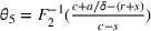
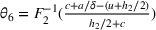
In period 2, the optimal decisions satisfy: (1) if
$\frac{a}{δ} \leq R_{2} (r)$
, then the optimal
${\hat{x}}_{2} + I = 0$
and
${\hat{y}}_{2} = 0$
; (2) if
$\frac{a}{δ} \geq R_{1} (r)$
, then the optimal
$({\hat{x}}_{2}, {\hat{y}}_{2})$
under the capability‐based system is the same as
$({\tilde{x}}_{2}, {\tilde{y}}_{2})$
under the capacity‐based system as given by Lemma 2; (3) if
$\frac{a}{δ} \in (R_{2} (r), R_{1} (r))$
, and (a)
if
$r \leq u + \frac{h_{2}}{2} - s$
, then
${\hat{x}}_{2} + I = 0$
and
${\hat{y}}_{2} = θ_{5}$
;
(b)
if
$r \in (u + \frac{h_{2}}{2} - s, \frac{(p - s) (h_{2} + u)}{p + h_{2} / 2})$
, then
${\hat{x}}_{2} + I = θ_{2}$
and
${\hat{y}}_{2} = θ_{5} - θ_{2}$
when
$\frac{a}{δ} \geq \frac{r (c + h_{2} / 2) - (c - s) (h_{2} + u)}{h_{2} / 2 + s}$
; while
${\hat{x}}_{2} + I = θ_{6}$
and
${\hat{y}}_{2} = 0$
when
$\frac{a}{δ} < \frac{r (c + h_{2} / 2) - (c - s) (h_{2} + u)}{h_{2} / 2 + s}$
;
(c)
if
$r \geq \frac{(p - s) (h_{2} + u)}{p + h_{2} / 2}$
, then
${\hat{x}}_{2} + I = θ_{6}$
and
${\hat{y}}_{2} = 0$
.
Also, when
$\frac{a}{δ} < R_{1} (r)$
, the shortfall probability and the expected shortfall of period 2 under capability‐based system can be expressed as:
$\begin{matrix} P {M_{2} \geq {\hat{x}}_{2} + I + {\hat{y}}_{2} + δ \hat{z}} & = & \frac{a}{(p - c) δ}, \\ E [{(M_{2} - ({\hat{x}}_{2} + I + {\hat{y}}_{2} + δ \hat{z}))}^{+}] & = & \int_{θ_{4}}^{+ \infty} (1 - F_{2} (m_{2})) d m_{2} . \end{matrix}$
17
However, when
$\frac{a}{δ} \geq R_{1} (r)$
, the shortfall probability and the expected shortfall of period 2 under capability‐based system are as same as the capacity‐based system as stated in the second statement of Proposition 2.

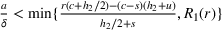
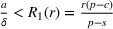
The first statement of Proposition 3 implies that in period 1, the optimal stockpile inventory and backup capacity under the capability‐based system are the same as under the capacity‐based system. This result is because it takes the entire period 1 to convert the capability to capacity, which can only be used in period 2. Hence, the shortfall probability and the expected shortfall of period 1 under the capability‐based system are the same as under the capacity‐based system.

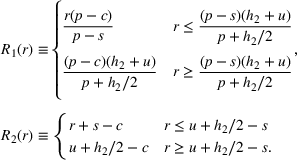
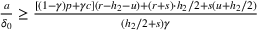
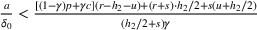
Next, we use Figure 4 to illustrate the optimal capability
$\hat{z}$
to be established in period 1 together with the optimal inventory and capacity
$({\hat{x}}_{2}, {\hat{y}}_{2})$
to be deployed in period 2. Proposition 3 and Figure 4 characterize the trade‐off among three resources z, x ₂, and y ₂. The first statement of Proposition 3 implies that the standby capability z is not needed when
$\frac{a}{δ}$
is sufficiently high (i.e., when
$\frac{a}{δ} \geq R_{1} (r)$
). Hence, when
$\hat{z} = 0$
, the trade‐off between the inventory x ₂ and capacity y ₂ of period 2 is the same as the capacity‐based system. This is as shown in the top portion of Figure 4. This result is due to the fact that
$\frac{a}{δ}$
captures the effective developing cost of the standby capability z, which is high when the developing cost of the standby capability a is high or the conversion rate δ is low. Hence, when
$\frac{a}{δ}$
is higher than
$R_{1} (r)$
, it is more economical to leverage the stockpile inventory x ₂ and backup capacity y ₂ in period 2 instead of developing the capability z in period 1.

FIGURE 4
Optimal
$\hat{z}$
of period 1 together the optimal
$({\hat{x}}_{2}, {\hat{y}}_{2})$
of period 2 under the capability‐based system

Statement 2 of Proposition 3 also suggests that, when
$\frac{a}{δ}$
is sufficiently low (i.e.,
$\frac{a}{δ} \leq R_{2} (r)$
), the stockpile inventory and the backup capacity of period 2 may not be needed (i.e.,
${\hat{x}}_{2} + I = {\hat{y}}_{2} = 0$
). This is because, with a low effective development cost, it is more economical for the government to develop the standby capability in period 1 and convert it to production capacity for use in period 2. This is as shown in the bottom right of Figure 4. Finally, when the effective development cost is moderate (i.e.,
$\frac{a}{δ} \in (R_{2} (r), R_{1} (r))$
), the government should develop standby capability in period 1 and convert it for capacity for use in period 2. Moreover, the government should also leverage some extra resources (stockpile inventory and/or backup capacity) in period 2, which depend on the reservation cost r. In particular, the government should develop a three‐tiered system that has
$\hat{z} > 0$
and
${\hat{x}}_{2}, {\hat{y}}_{2} > 0$
only when the backup capacity reservation cost r and the effective standby capability development cost
$\frac{a}{δ}$
are both moderate (as shown in the unshaded area in Figure 4).

Next, by focusing on the case when the government raises all three resources in period 1 (i.e.,
${\hat{x}}_{1}, {\hat{y}}_{1}, z > 0$
), we can compare the optimal government decisions across two periods as follows: Corollary 4
Suppose the capacity reservation cost
$r \in (u + h_{1} / 2 - s, \frac{h_{1} (p - s)}{p - u + h_{1} / 2})$
and the effective capability developing cost
$\frac{a}{δ} < R_{1} (r)$
so that all three resources (inventory, capacity, capability) would be developed in period 1 under the capability‐based system. Then, (1)
the shortfall probability in period 1 is higher than that of period 2, that is,
$P {M_{1} \geq {\hat{x}}_{1} + {\hat{y}}_{1}} = \frac{r}{p - s} > P {M_{2} \geq {\hat{x}}_{2} + I + {\hat{y}}_{2} + δ \hat{z}} = \frac{a}{(p - c) δ}$
;
(2)
if the demand distribution is the same in both periods (i.e.,
$F_{1} (\cdot) = F_{2} (\cdot)$
), then the optimal stockpile inventory
${\hat{x}}_{1} > {\hat{x}}_{2}$
and the total amount of inventory and capacity
${\hat{x}}_{1} + {\hat{y}}_{1} > {\hat{x}}_{2} + {\hat{y}}_{2}$
. Also, the expected shortfall in period 2 is smaller than that of period 1, that is,
$E [{(M_{2} - ({\hat{x}}_{2} + I + {\hat{y}}_{2} + δ \hat{z}))}^{+}] < E [{(M_{1} - ({\hat{x}}_{1} + {\hat{y}}_{1}))}^{+}]$
.

When the reservation cost r of the backup capacity is moderate and the effective capability developing cost
$\frac{a}{δ}$
is below
$R_{1} (r)$
so that the government would leverage all three resources in period 1, Corollary 4 generates new results that are different from those under the inventory‐based system (Corollary 1) and capacity‐based system (Corollary 2) as follows. First, under the capability‐based system, statement 1 asserts that the shortfall probability of period 2 is lower than period 1 regardless of the demand distribution. Compared to the previous two systems, the capability‐based system provides an extra option—production capacity
$δ z$
converted from standby capability developed in period 1. This additional capacity can be used for period 2 to further reduce the shortfall probability. Also, when the demand distributions for both periods are the same, statement 2 reveals that it is optimal for the government to set a higher stockpile inventory level (i.e.,
${\hat{x}}_{1}$
) in period 1, ensuring a higher level of the total stockpile inventory and backup capacity (i.e.,
${\hat{x}}_{1} + {\hat{y}}_{1}$
) in period 1. Also, when the capability developed in period 1 can only be used in period 2 and when the inventory in period 1 can be carried over to period 2, the expected shortfall of period 2 is lower than that of period 1.

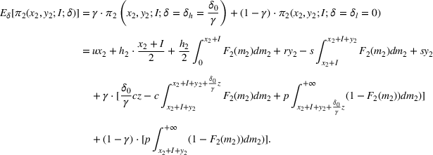
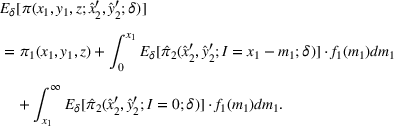
Comparing capability‐ and capacity‐based systems

We now compare the optimal capacity‐based system and the optimal capability‐based system by comparing the results in Propositions 2 and 3. Corollary 5
Relative to the optimal capacity‐based system
$({\tilde{x}}_{1}, {\tilde{y}}_{1}, 0; {\tilde{x}}_{2}, {\tilde{y}}_{2})$
, the optimal capability‐based system
$({\hat{x}}_{1}, {\hat{y}}_{1}, \hat{z}; {\hat{x}}_{2}, {\hat{y}}_{2})$
possesses the following properties: (1)
Stockpile inventory. In period 1, the inventory level under the capability‐based system is the same as that under the capacity‐based system (i.e.,
${\hat{x}}_{1} = {\tilde{x}}_{1}$
). In period 2, given the same left‐over inventory I, less inventory is needed under the capability‐based system (i.e.,
${\hat{x}}_{2} < {\tilde{x}}_{2}$
) if and only if the capacity reservation cost
$r > u + h_{2} / 2 - s$
and the effective capability development cost
$\frac{a}{δ} < \min {\frac{r (c + h_{2} / 2) - (c - s) (h_{2} + u)}{h_{2} / 2 + s}, R_{1} (r)}$
.
(2)
Backup capacity. In period 1, the capacity level under the capability‐based system is the same as that under the capacity‐based system, (i.e.,
${\hat{y}}_{1} = {\tilde{y}}_{1}$
). In period 2, less capacity is needed under the capability‐based system (i.e.,
${\hat{y}}_{2} < {\tilde{y}}_{2}$
) if and only if the capacity reservation cost
$r < \frac{(p - s) (h_{2} + u)}{p + h_{2} / 2}$
and the effective capability development cost
$\frac{a}{δ} < R_{1} (r) = \frac{r (p - c)}{p - s}$
.
(3)
Shortfall probability and expected shortfall. In period 1, both the shortfall probability and the expected shortfall under the capability‐based system are the same as those under the capacity‐based system (i.e.,
$P {M_{1} \geq {\hat{x}}_{1} + {\hat{y}}_{1}} = P {M_{1} \geq {\tilde{x}}_{1} + {\tilde{y}}_{1}}$
and
$E [{(M_{1} - ({\hat{x}}_{1} + {\hat{y}}_{1}))}^{+}] = E [{(M_{1} - ({\tilde{x}}_{1} + {\tilde{y}}_{1}))}^{+}]$
). In period 2, the shortfall probability and the expected shortfall under the capability‐based system are both strictly lower than those under the capacity‐based system (i.e.,
$P {M_{2} \geq {\hat{x}}_{2} + I + {\hat{y}}_{2} + δ \hat{z}} < P {M_{2} \geq {\tilde{x}}_{2} + I + {\tilde{y}}_{2}}$
and
$E [{(M_{2} - ({\hat{x}}_{2} + I + {\hat{y}}_{2} + δ \hat{z}))}^{+}] < E [{(M_{2} - ({\tilde{x}}_{2} + I + {\tilde{y}}_{2}))}^{+}]$
) if and only if the effective capability development cost
$\frac{a}{δ} < R_{1} (r)$
.
(4)
Expected relevant cost. The capability‐based system incurs a strictly lower total relevant cost than the capacity‐based system (i.e.,
$π ({\hat{x}}_{1}, {\hat{y}}_{1}, \hat{z}; {\hat{x}}_{2}, {\hat{y}}_{2}) < π ({\tilde{x}}_{1}, {\tilde{y}}_{1}, 0; {\tilde{x}}_{2}, {\tilde{y}}_{2})$
) if and only if the effective capability
$\frac{a}{δ} < R_{1} (r)$
.

Corollary 5 has the following implications. First, because there is an extra option (converted production capacity
$δ z$
from standby capability developed in period 1) can be used to satisfy the demand in period 2, the capability‐based system can enable the government to reduce the relevant cost only when the effective development cost
$\frac{a}{δ} < R_{1} (r)$
. This is as stated in statement 4 of Corollary 5. Next, even though there is an extra option to develop capability, statement 3 reveals that the capability‐based system can reduce the shortfall probability and the expected shortfalls in period 2 only when the effective development cost
$\frac{a}{δ} < R_{1} (r)$
. The condition
$\frac{a}{δ} < R_{1} (r)$
is depicted in the shaded area of Figure 5c within which the capability‐based system outperforms the capacity‐based system in terms of the total cost, shortfall probability, and expected shortfall as captured in statements 3 and 4.

FIGURE 5
Comparison: Capability‐based and capacity‐based systems. (a) Comparison: Stockpile inventory in period 2. (b) Comparison: Backup capacity in period 2. (c) Comparison: Shortfall probability and expected shortfall in period 2 and expected total cost

Statements 1 and 2 of Corollary 5 offer the following insights. Statement 1 states that the capability‐based system can result in a lower inventory level in period 2 than that of the capacity‐based system only when the capacity reservation cost
$r > (u + h_{2} / 2 - s)$
and the effective capability development cost
$\frac{a}{δ} < R_{1} (r)$
(as illustrated in the shaded area of Figure 5a). This result can be explained as follows. When the capacity reservation cost r is too low, the stockpile inventory is less economical than the backup capacity so that the government will always set the inventory level to be zero under both capacity‐based and capability‐based systems. Hence, the government will leverage the stockpile inventory only when the capacity reservation cost r is above a certain threshold. Second, when the effective capability development cost
$\frac{a}{δ}$
is sufficiently low, it is more economical for the government to develop more standby capability in period 1 and convert it for use in period 2 so as to reduce the stockpile inventory level in period 2.

Finally, Statement 2 of Corollary 5 states that the capability‐based system can result in a lower capacity level in period 2 than that of the capacity‐based system only when both the capacity reservation cost r and the effective capability development cost
$\frac{a}{δ}$
are below certain thresholds. It is because, when the capacity reservation cost r is too high, capacity is not economical under both capacity‐based and capability‐based systems. Hence, the government will leverage the backup capacity only when r is below a certain threshold. Also, when the effective capability development cost
$\frac{a}{δ}$
is sufficiently low, it is more economical for the government to develop more standby capability in period 1 and convert it for use in period 2 so as to reduce the backup capacity levels in period 2. This is illustrated in the shaded area of Figure 5b.

UNCERTAIN CAPABILITY CONVERSION YIELD

Recall from Subsection 4.3 that the yield δ for converting the standby capability z is deterministic. However, when the capability is based on unproven R&D technologies, the conversion yield δ is likely to be uncertain. We now extend our analysis to the case when the conversion yield δ is uncertain. For tractability, we assume that the conversion yield δ follows a two‐point distribution, one point representing failed conversion. as with an unproven technology, for instance, in converting biotech R&D projects into drugs for FDA approval. (We will numerically examine the case when the conversion does not fail in either case.)

We assume that the conversion yield
$δ = δ_{h}$
with probability γ and the conversion would fail with
$δ = δ_{l} = 0$
with probability
$(1 - γ)$
. Define the term
$δ_{0} = γ \cdot δ_{h}$
so that we can express
$δ_{h} = δ_{0} / γ$
. In doing so, the expected conversion yield is equal to δ₀ because
$γ δ_{h} + (1 - γ) δ_{l} = δ_{0}$
. (Observe that when
$γ = 1$
, this case reduces to the base model where the deterministic yield rate
$δ = δ_{0}$
.)

Because uncertain yield δ affects the capability z primarily, it suffices to focus our analysis on the capability‐based system
$(x_{1}, y_{1}, z; x_{2}, y_{2})$
. To proceed, let us first analyze period 2's problem.

Period 2. For any realized yield δ associated with capability z established in period 1, the ex post relevant cost
$π_{2} (x_{2}, y_{2}; I; δ)$
in period 2 associated with any given decision
$(x_{2}, y_{2})$
and leftover inventory I is as given in (13). Hence, when δ is still uncertain at the beginning of period 2, the ex ante expected relevant cost of period 2 is
$E_{δ} [π_{2} (x_{2}, y_{2}; I; δ)]$
, where:
$\begin{matrix} E_{δ} [π_{2} (x_{2}, y_{2}; I; δ)] = & γ \cdot π_{2} (x_{2}, y_{2}; I; δ = δ_{h} = \frac{δ_{0}}{γ}) + (1 - γ) \cdot π_{2} (x_{2}, y_{2}; I; δ = δ_{l} = 0) \\ = & u x_{2} + h_{2} \cdot \frac{x_{2} + I}{2} + \frac{h_{2}}{2} \int_{0}^{x_{2} + I} F_{2} (m_{2}) d m_{2} + r y_{2} - s \int_{x_{2} + I}^{x_{2} + I + y_{2}} F_{2} (m_{2}) d m_{2} + s y_{2} \\ + γ \cdot [\frac{δ_{0}}{γ} c z - c \int_{x_{2} + I + y_{2}}^{x_{2} + I + y_{2} + \frac{δ_{0}}{γ} z} F_{2} (m_{2}) d m_{2} + p \int_{x_{2} + I + y_{2} + \frac{δ_{0}}{γ} z}^{+ \infty} (1 - F_{2} (m_{2})) d m_{2})] \\ + (1 - γ) \cdot [p \int_{x_{2} + I + y_{2}}^{+ \infty} (1 - F_{2} (m_{2})) d m_{2})] . \end{matrix}$
18
By noting that
$\frac{\partial E_{δ} [π_{2} (x_{2}, y_{2}; I; δ)]}{\partial x_{2}}$
and
$\frac{\partial E_{δ} [π_{2} (x_{2}, y_{2}; I; δ)]}{\partial y_{2}}$
resemble that of the base model, the optimal
$({\hat{x}}_{2}^{'}, {\hat{y}}_{2}^{'})$
would also depend on the capability level z established in period 1.

Period 1's problem. Because the standby capability cannot be converted for use in period 1, the expected relevant cost of period 1
$π_{1} (x_{1}, y_{1}, z)$
is the same as in the base case as stated in (14). Hence, by incorporating the optimal expected cost in period 2 based on
$({\hat{x}}_{2}^{'}, {\hat{y}}_{2}^{'})$
given in (18), the total relevant ex ante expected relevant cost over both periods can be expressed as:
$\begin{matrix} E_{δ} [π (x_{1}, y_{1}, z; {\hat{x}}_{2}^{'}, {\hat{y}}_{2}^{'}; δ)] \\ = π_{1} (x_{1}, y_{1}, z) + \int_{0}^{x_{1}} E_{δ} [{\hat{π}}_{2} ({\hat{x}}_{2}^{'}, {\hat{y}}_{2}^{'}; I = x_{1} - m_{1}; δ)] \cdot f_{1} (m_{1}) d m_{1} \\ + \int_{x_{1}}^{\infty} E_{δ} [{\hat{π}}_{2} ({\hat{x}}_{2}^{'}, {\hat{y}}_{2}^{'}; I = 0; δ)] \cdot f_{1} (m_{1}) d m_{1} . \end{matrix}$
19
Observe that (19) resembles (15). Hence, it is easy to check that the optimal
$({\hat{x}}_{1}^{'}, {\hat{y}}_{1}^{'})$
is the same as the base case with a fixed yield rate, which is characterized in Proposition 3.

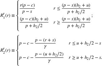
Optimal decisions under uncertain conversion yield

To derive the optimal decisions
${\hat{z}}^{'}$
and
$({\hat{x}}_{2}^{'}, {\hat{y}}_{2}^{'})$
, we need to differentiate
$E_{δ} [π (x_{1}, y_{1}, z; {\hat{x}}_{2}, {\hat{y}}_{2}; δ)]$
with respect to z, and by also considering the first order derivatives of
$E_{δ} [π_{2} (x_{2}, y_{2}; I; δ)]$
with respect to x ₂ and y ₂ as given in Equations (EC.3) and (EC.4) in the Supporting Information. Analogous to the base case and in preparation, let
$θ_{4}^{'} = F_{2}^{- 1} (\frac{(p - c) - a / δ_{0}}{p - c})$
,
$θ_{5}^{'} = F_{2}^{- 1} (\frac{(1 - γ) p + γ (c + a / δ_{0}) - (r + s)}{(c - s) + (1 - γ) (p - c)})$
, and
$θ_{6}^{'} = F_{2}^{- 1} (\frac{(1 - γ) p + γ (c + a / δ_{0}) - (u + h_{2} / 2)}{(h_{2} / 2 + c) + (1 - γ) (p - c)})$
. It is easy to check that
$θ_{4}^{'}$
is independent of γ, while
$θ_{5}^{'}$
and
$θ_{6}^{'}$
are decreasing in γ. Also, we define two new thresholds
$R_{1}^{'} (r)$
and
$R_{2}^{'} (r)$
, where:
$\begin{matrix} R_{1}^{'} (r) \equiv \{\begin{matrix} \frac{r (p - c)}{p - s} & r \leq \frac{(p - s) (h_{2} + u)}{p + h_{2} / 2} \\ \frac{(p - c) (h_{2} + u)}{p + h_{2} / 2} & r \geq \frac{(p - s) (h_{2} + u)}{p + h_{2} / 2} \end{matrix}; \\ R_{2}^{'} (r) \equiv \{\begin{matrix} p - c - \frac{p - (r + s)}{γ} & r \leq u + h_{2} / 2 - s \\ p - c - \frac{p - (u + h_{2} / 2)}{γ} & r \geq u + h_{2} / 2 - s . \end{matrix} \end{matrix}$
20
Observe that
$R_{1}^{'} (r)$
and
$R_{2}^{'} (r)$
are analogous to
$R_{1} (r)$
and
$R_{2} (r)$
as in the base model. Specifically, while
$R_{1}^{'} (r)$
is independent of γ,
$R_{2}^{'} (r)$
is increasing in γ. By using these two thresholds, we can characterize the optimal government decision
$({\hat{x}}_{1}^{'}, {\hat{y}}_{1}^{'}, {\hat{z}}^{'}; {\hat{x}}_{2}^{'}, {\hat{y}}_{2}^{'})$
with uncertain yield as follows. Proposition 4 Capability‐based system with uncertain yield

Under the capability‐based system with uncertain conversion yield so that

δ = δ_{h} = δ_{0} / γ

with probability γ (

γ \in (0, 1]

) and

δ = δ_{l} = 0

with probability

1 - γ

, the optimal decision

({\hat{x}}_{1}^{'}, {\hat{y}}_{1}^{'}, {\hat{z}}^{'}; {\hat{x}}_{2}^{'}, {\hat{y}}_{2}^{'})

can be described as follows:

(1)

In period 1, the optimal inventory

{\hat{x}}_{1}^{'}

and optimal capacity

{\hat{y}}_{1}^{'}

are the same as the optimal

{\hat{x}}_{1}

and

{\hat{y}}_{1}

for the base model as stated in Proposition 3 (when we set the fixed yield

δ = δ_{0}

, where δ₀ is the expected yield in the uncertain yield case). Also, the optimal capability

{\hat{z}}^{'}

satisfies:

(a)

\frac{a}{δ_{0}} \geq R_{1}^{'} (r)

, then

{\hat{z}}^{'} = 0

;

(b)

\frac{a}{δ_{0}} \in (R_{2}^{'} (r), R_{1}^{'} (r))

, then

0 < {\hat{z}}^{'} < \frac{θ_{4}^{'}}{δ_{0} / γ}

. Specifically,

(i)

\frac{a}{δ_{0}} \geq \frac{[(1 - γ) p + γ c] (r - h_{2} - u) + (r + s) \cdot h_{2} / 2 + s (u + h_{2} / 2)}{(h_{2} / 2 + s) γ}

{\hat{z}}^{'} = \frac{1}{δ_{0} / γ} (θ_{4}^{'} - θ_{5}^{'})

and

{\hat{z}}^{'}

is increasing in γ;

(ii)

\frac{a}{δ_{0}} \leq \frac{[(1 - γ) p + γ c] (r - h_{2} - u) + (r + s) \cdot h_{2} / 2 + s (u + h_{2} / 2)}{(h_{2} / 2 + s) γ}

{\hat{z}}^{'} = \frac{1}{δ_{0} / γ} (θ_{4}^{'} - θ_{6}^{'})

and

{\hat{z}}^{'}

is increasing in γ;

(c)

\frac{a}{δ_{0}} \leq R_{2}^{'} (r)

, then

{\hat{z}}^{'} = \frac{θ_{4}^{'}}{δ_{0} / γ}

and

{\hat{z}}^{'}

is increasing in γ.

(2)

In period 2, the optimal decisions satisfy: (1) if

\frac{a}{δ_{0}} \leq R_{2}^{'} (r)

, then the optimal

{\hat{x}}_{2}^{'} + I = 0

and

{\hat{y}}_{2}^{'} = 0

; (2) if

\frac{a}{δ_{0}} \geq R_{1}^{'} (r)

, then the optimal

({\hat{x}}_{2}^{'}, {\hat{y}}_{2}^{'})

is the same as

({\tilde{x}}_{2}, {\tilde{y}}_{2})

under the capacity‐based system as given by Lemma 2; (3) if

\frac{a}{δ_{0}} \in (R_{2}^{'} (r), R_{1}^{'} (r))

, we have the following three cases:

(a)

r \leq u + \frac{h_{2}}{2} - s

, then

{\hat{x}}_{2}^{'} + I = 0

{\hat{y}}_{2}^{'} = θ_{5}^{'}

and

{\hat{y}}_{2}^{'}

is decreasing in γ.

(b)

r \in (u + \frac{h_{2}}{2} - s, \frac{(p - s) (h_{2} + u)}{p + h_{2} / 2})

, then:

(i)

when

\frac{a}{δ_{0}} \geq \frac{[(1 - γ) p + γ c] (r - h_{2} - u) + (r + s) \cdot h_{2} / 2 + s (u + h_{2} / 2)}{(h_{2} / 2 + s) γ}

{\hat{x}}_{2}^{'} + I = θ_{2}

{\hat{y}}_{2}^{'} = θ_{5}^{'} - θ_{2}

{\hat{x}}_{2}^{'}

is independent of γ, and

{\hat{y}}_{2}^{'}

is decreasing in γ; and

(ii)

when

\frac{a}{δ_{0}} < \frac{[(1 - γ) p + γ c] (r - h_{2} - u) + (r + s) \cdot h_{2} / 2 + s (u + h_{2} / 2)}{(h_{2} / 2 + s) γ}

{\hat{x}}_{2}^{'} + I = θ_{6}^{'}

{\hat{y}}_{2}^{'} = 0

, and

{\hat{x}}_{2}^{'}

is decreasing in γ.

(c)

r \geq \frac{(p - s) (h_{2} + u)}{p + h_{2} / 2}

, then

{\hat{x}}_{2}^{'} + I = θ_{6}^{'}

{\hat{y}}_{2}^{'} = 0

, and

{\hat{x}}_{2}^{'}

is decreasing in γ.

Proposition 4 resembles Proposition 3. Hence, the optimal government decision

({\hat{x}}_{1}^{'}, {\hat{y}}_{1}^{'}, {\hat{z}}^{'}; {\hat{x}}_{2}^{'}, {\hat{y}}_{2}^{'})

under uncertain yield possesses the same structure as in the base model when the fixed yield

δ = δ_{0}

, where δ₀ is the expected yield in the uncertain yield case.

To examine the impact of conversion yield uncertainty level γ on those optimal decisions

({\hat{x}}_{1}^{'}, {\hat{y}}_{1}^{'}, {\hat{z}}^{'}; {\hat{x}}_{2}^{'}, {\hat{y}}_{2}^{'})

as stated in Proposition 4, let us first observe from statement 1 asserting that conversion yield uncertainty has no impact on the optimal level of stockpile inventory and backup capacity

({\hat{x}}_{1}^{'}, {\hat{y}}_{1}^{'})

in period 1. This is because, the conversion process takes up the entire period 1, so the conversion outcome would not affect the optimal decisions in period 1.

We now examine the impact of yield uncertainty γ on the optimal decisions in period 2; namely, the optimal level of the standby capability

{\hat{z}}^{'}

determined in period 1, and the optimal inventory and capacity

({\hat{x}}_{2}^{'}, {\hat{y}}_{2}^{'})

in period 2. For ease of exposition, we use Figure 6 to illustrate Proposition 4. Here, panel (a) examines the case when

γ < 1

so that the yield rate is uncertain, and panel (b) deals with the benchmark case when

γ = 1

so that the yield rate is fixed (i.e.,

δ = δ_{0}

).¹⁴

FIGURE 6

Comparison: Optimal government decisions on z and

(x_{2}, y_{2})

. (a)

γ < 1

so that the yield rate is uncertain. (b)

γ = 1

so that the yield rate is fixed at δ₀.

First, recall from above that

R_{1}^{'} (r)

is independent of γ and that

R_{1}^{'} (r) = R_{1} (r)

. This observation and statement 1(a) imply that, when

\frac{a}{δ_{0}} \geq R_{1}^{'} (r)

{\hat{z}}^{'} = 0

. This result implies that, when the fixed unit cost a for developing capability is high or when the expected conversion yield δ₀ is low so that

\frac{a}{δ_{0}} \geq R_{1}^{'} (r)

, developing capability is never optimal. Also, because

R_{1}^{'} (r)

is independent of yield uncertainty γ, this condition is also independent of γ, which explains why the regions for

{\hat{z}}^{'} = 0

(i.e., zones # 1, 4, and 7) in both panels of Figure 6 are not affected by γ.

Next, recall from above that the threshold

R_{2}^{'} (r)

is increasing in γ. This observation along with statement 1 and statement 2(1) (i.e., when

\frac{a}{δ_{0}} \leq R_{2}^{'} (r)

) explains why the region for

{\hat{z}}^{'} > 0, {\hat{x}}_{2}^{'} + I = 0

and

{\hat{y}}_{2}^{'} = 0

as depicted in zone #3 would “expand” as γ (i.e., as conversion yield uncertainty) increases, which is evident when we compare the size of zone #3 between panel (b) and panel (a) in Figure 6. In other words, when the fixed unit cost a for developing capacity is low or when the expected yield δ₀ is high so that

\frac{a}{δ_{0}} \leq R_{2}^{'} (r)

, it is optimal (i.e., more cost‐effective) for the government to develop and convert capability without the need to leverage any stockpile inventory and backup capacity in period 2.

Finally, by using the process of elimination, it is easy to observe the remaining zones # 2, 5, 6 in Figure 6 would “contract” as γ increases (through a direct comparison between panel (b) and panel (a)). This implies that, when the conversion yield is uncertain (i.e., as γ decreases), it is more likely that the government should leverage stockpile inventory and/or backup capacity in period 2 in addition to using the converted capability.

Impact of uncertain conversion yield

By focusing on the case when

\frac{a}{δ_{0}} < R_{1}^{'} (r)

so that the standby capability is needed (i.e., when

{\hat{z}}^{'} > 0

),¹⁵ we can use the results stated in Proposition 4 to examine the impact of yield uncertainty γ on the optimal government decision on

{\hat{z}}^{'}

and

({\hat{x}}_{2}^{'}, {\hat{y}}_{2}^{'})

. To do so, we first use the base model to establish a “benchmark case” by setting the fixed yield

δ = δ_{0}

. Then, because the “expected yield” in the uncertain yield case is equal to δ₀, we can compare the results as stated in Propositions 4 and 3 to examine the impact of conversion yield uncertainty (γ) on the optimal decisions. Corollary 6 summarizes our findings based on this direct comparison. Corollary 6

Suppose

\frac{a}{δ_{0}} < R_{1}^{'} (r)

so that the government will leverage the standby capability in period 1 (i.e.,

{\hat{z}}^{'} > 0

). Then, relative to the optimal capability‐based system

({\hat{x}}_{1}, {\hat{y}}_{1}, \hat{z}; {\hat{x}}_{2}, {\hat{y}}_{2})

for the base case with a fixed yield rate δ₀, the optimal capability‐based system

({\hat{x}}_{1}^{'}, {\hat{y}}_{1}^{'}, {\hat{z}}^{'}; {\hat{x}}_{2}^{'}, {\hat{y}}_{2}^{'})

for the case when the yield rate δ is uncertain (with probability

γ < 1

δ = δ_{h} = δ_{0} / γ

and with probability

1 - γ > 0

δ = δ_{l} = 0

so that the expected yield equals δ₀) possesses the following properties:

(1)

Stockpile inventory. In period 1, yield uncertainty has no impact on the optimal inventory level, that is,

{\hat{x}}_{1}^{'} = {\hat{x}}_{1}

. In period 2, given the same leftover inventory I, when capacity is reserved in period 2 (i.e.,

{\hat{y}}_{2} > 0

{\hat{x}}_{2}^{'} = {\hat{x}}_{2}

so that yield uncertainty has no impact on the optimal inventory level. However, when no capacity is reserved in period 2 (i.e.,

{\hat{y}}_{2} = 0

{\hat{x}}_{2}^{'} \geq {\hat{x}}_{2}

so that yield uncertainty creates the need to stock more in period 2.

(2)

Backup capacity. In period 1, yield uncertainty has no impact on the reserved capacity level, that is,

{\hat{y}}_{1}^{'} = {\hat{y}}_{1}

. However, in period 2,

{\hat{y}}_{2}^{'} \geq {\hat{y}}_{2}

so that yield uncertainty creates the need to reserve a higher capacity in period 2.

(3)

Standby capability. In period 1,

{\hat{z}}^{'} \leq \hat{z}

. Hence, conversion yield uncertainty creates negative incentives. It is optimal for the government to develop a lower standby capability level in period 1.

(4)

Shortfall probability and expected shortfall. In period 1, yield uncertainty has no impact on the shortfall probability and expected shortfall, that is,

P {M_{1} \geq {\hat{x}}_{1}^{'} + {\hat{y}}_{1}^{'}} = P {M_{1} \geq {\hat{x}}_{1} + {\hat{y}}_{1}}

and

E [{(M_{1} - ({\hat{x}}_{1}^{'} + {\hat{y}}_{1}^{'}))}^{+}] = E [{(M_{1} - ({\hat{x}}_{1} + {\hat{y}}_{1}))}^{+}]

. However, in period 2, the shortfall probability and the expected shortfall are both higher for the case when the yield rate is uncertain, that is,

P {M_{2} \geq ({\hat{x}}_{2}^{'} + I + {\hat{y}}_{2}^{'} + δ {\hat{z}}^{'})} > P {M_{2} \geq {\hat{x}}_{2} + I + {\hat{y}}_{2} + δ_{0} \hat{z}} = \frac{a}{δ_{0} (p - c)}

and

E [{(M_{2} - ({\hat{x}}_{2}^{'} + I + {\hat{y}}_{2}^{'} + δ {\hat{z}}^{'}))}^{+}] > E [{(M_{2} - ({\hat{x}}_{2} + I + {\hat{y}}_{2} + δ_{0} \hat{z}))}^{+}] = \int_{θ_{4}^{'}}^{+ \infty} (1 - F_{2} (m_{2})) d m_{2}

Corollary 6 reveals the impact of conversion yield uncertainty on inventory, capacity, and capability. First, under favorable conditions for developing capability (i.e., when

\frac{a}{δ_{0}} < R_{1}^{'} (r)

as stated in statement 1 of Proposition 4), the conversion yield uncertainty has no impact on the optimal decisions in period 1. However, uncertain conversion yield creates additional incentives for the government to order more inventory and reserve a higher capacity in period 2. At the same time, uncertain conversion yield discourages the government to develop more capability. Also, the last statement of Corollary 6 implies that conversion yield uncertainty would generate a higher shortfall.

Numerical study

We have obtained analytical results for the case when the capability conversion may fail; that is,

δ = δ_{l} = 0

with probability

(1 - γ)

. However, the analysis for the general case when the conversion would never fail completely (i.e., when

δ_{l} > 0

) is mathematically intractable. For this reason, we conduct numerical analysis to examine the impact of uncertain conversion yield on the optimal decisions regarding inventory, capacity, and capability for the general case.

We construct our numerical study of the general case based on the following two‐point distribution: with probability

(1 - γ)

δ = δ_{l} \equiv d

(where d is a parameter); and with probability γ,

δ = δ_{h} \equiv \frac{δ_{0}}{γ} - \frac{1 - γ}{γ} d

. To ensure

δ_{l} < δ_{h}

, the parameter

d < δ_{0}

. Using this setup, it is easy to check that the expected yield equals

δ_{0} = γ δ_{h} + (1 - γ) δ_{l}

. Hence, our general case will reduce to our extension case in Section 5 when

d = 0

, and this general case will further reduce to our base model (with deterministic yield

δ = δ_{0}

) when

d = 0

and

γ = 1

. By using this setup, we can compare our results for the general case against the base model numerically.

Because it takes period 1 to convert the standby capability, we can use the same approach presented in Section 5.1 to show analytically that the inventory and capacity in period 1 (i.e.,

{\hat{x}}_{1}^{'}

and

{\hat{y}}_{1}^{'}

) are the same as that of the base model as stated in Proposition 3 for the general case. Therefore, it suffices to conduct our numerical study by focusing on the optimal decisions regarding the inventory

{\hat{x}}_{2}^{'}

and capacity

{\hat{y}}_{2}^{'}

in period 2, and the optimal capability

{\hat{z}}^{'}

in period 1.

Our setup for the general case enables us to compare our numerical results and analytical results in a consistent manner. To elaborate, observe that the “gap”; that is,

(δ_{h} - δ_{l})

, between the higher yield

δ_{h} = \frac{δ_{0}}{γ} - \frac{1 - γ}{γ} d

and the lower yield

δ_{l} = d

becomes “narrower” when the lower yield rate d increases or when the chance of getting the higher yield rate γ increases. Therefore, as d or γ increases, the level of conversion uncertainty decreases. Thus, by varying the values of d and γ, we can examine the impact of uncertainty level on the optimal inventory and capacity

{\hat{x}}_{2}^{'}, {\hat{y}}_{2}^{'}

in period 2 and the optimal capability

{\hat{z}}^{'}

in period 1.

We conducted the numerical analysis by setting the cost components

(u, h_{2}) = (900, 600)

(r, s) = (500, 1100)

(a, c) = (200, 1200)

, and

p = 2000

, and the expected yield

δ_{0} = 0.5

. In Figure 7, we report the optimal decisions

{\hat{x}}_{2}^{'}, {\hat{y}}_{2}^{'}

and

{\hat{z}}^{'}

for the general case based on two sets of numerical experiments: (1) we set

γ = 0.5

and vary d from 0 to δ₀; and (2) we set

d = 0.3

and vary γ from 0.001 to 1. Also, we establish benchmarks in Figure 7 by plotting the optimal decisions

{\hat{x}}_{2}, {\hat{y}}_{2}

, and

\hat{z}

for the base model (with deterministic yield

δ = δ_{0}

) by using the results as stated in Proposition 3. We also conducted numerical experiments using different parameter values. The structural results remain the same and are omitted.

FIGURE 7

Numerical comparison. (a) The impact of the lower yield rate d on the optimal decisions regarding the inventory

{\hat{x}}_{2}^{'}

and capacity

{\hat{y}}_{2}^{'}

in period 2, and the capability

{\hat{z}}^{'}

in period 1. (b) The impact of the probability of getting the high conversion yield γ on the optimal decisions regarding the inventory

{\hat{x}}_{2}^{'}

and capacity

{\hat{y}}_{2}^{'}

in period 2, and the capability

{\hat{z}}^{'}

in period 1

By comparing the values of

{\hat{x}}_{2}^{'}, {\hat{y}}_{2}^{'}

, and

{\hat{z}}^{'}

for the general case against their corresponding benchmarks

{\hat{x}}_{2}, {\hat{y}}_{2}

, and

\hat{z}

for the base model as shown in both panels of Figure 7, we find that

{\hat{x}}_{2}^{'} \geq {\hat{x}}_{2}, {\hat{y}}_{2}^{'} \geq {\hat{y}}_{2}

and

{\hat{z}}^{'} \leq \hat{z}

. This numerical result reveals that our analytical results as stated in Corollary 6 established for the special case that has

d = 0

continue to hold for the general case that has

d > 0

as shown in Figure 7a. Also, we obtain consistent results for different values of γ as shown in Figure 7b. Therefore, the results stated in Corollary 6 continue to hold for the general case: when the yield conversion becomes uncertain, it is optimal for the government to increase the inventory and capacity levels in period 2, and reduce the capability level in period 1.

Finally, recall that the level of yield conversion uncertainty is decreased when d or γ increases. Observe from Figure 7a,b that the optimal inventory

{\hat{x}}_{2}^{'}

and capacity

{\hat{y}}_{2}^{'}

are decreasing, whereas the optimal capability level

{\hat{z}}^{'}

is increasing when d or γ increases. Hence, when the level of conversion yield uncertainty decreases, the government can afford to leverage capability more and rely on inventory and capacity less.

CONCLUSION

Drawing lessons from the shortcomings of the inventory‐based national stockpiles during the COVID‐19 pandemic, we examined if and when how a proactive three‐tiered integrating stockpile inventory, backup capacity, and standby capability would perform. By analyzing a two‐period model, we obtained the following main results: (1) Adding capacity to inventory can reduce inventory that can become obsolete, reduce the shortfall probability, and reduce the total expected cost. (2) Adding capability in period 1 lowers the shortfall probability in period 2 due to the additional converted capacity that becomes available, and it can be more cost‐effective. (3) capability conversion uncertainty necessitates more inventory and reserved capacity in period 2, while creating a disincentive for developing more capability in period 1.

We mapped out our main results by successively adding capacity and capability successively to the inventory‐only system. Doing so allowed us to compare the incremental benefit by way of cost, expected shortfalls, and shortfall probability. This system performance evaluation can be useful for any public health government agency or humanitarian organization to develop an efficient response system by integrating all three resources (inventory, capacity, and capability) instead of treating them in isolation.

Our paper represents only an initial attempt to present, model, and analyze a three‐tiered integrated system via a two‐period model, and offers many opportunities for further research: (1)

Strategic humanitarian operations: Humanitarian operations deal with a pre‐positioned inventory to meet the needs if a large disaster of any size were to occur anywhere in the region under consideration. The natural question is how to deploy capacity and capability to bolster inventory (in different locations) for responding to disasters and recovering afterward.

(2)

A multi‐period view: Our model is a two‐period model, with the periods being notional and not necessarily equal in duration. We can change the model to multiple months or years (so that the time periods of equal length), particularly for slow‐onset disasters like droughts. Moreover, such an extension could incorporate the stockpile products perishing, or becoming obsolete. We could even consider a multi‐period view over days to include the spread of the pandemic with an epidemiology model like the Susceptible‐Infected‐and‐Recovered (SIR) model to predict demand.

(3)

Capability conversion yield: For tractability, we have considered the two‐point distribution to capture uncertain capability conversion yield. Besides the idea of exploring more general distributions, future research could examine whether (and how) the government should offer performance‐based subsidies to encourage research organizations to develop capability with a higher and/or a more reliable conversion yield.

(4)

Other views of capability: Our paper looks at capability only from the narrow viewpoint of being able to create manufacturing capacity only for the specific items needed for the pandemic. In reality, such capability entails building knowledge and job skills for producing a variety of products and services for multiple industries. Further research could also extend the idea of the flexibility of capacity to capability. See Chopra et al. (2021) for an argument about the flexibility afforded by “industrial commons.”

These ideas for future research indicate that viewing inventory, capacity, and capability in an integrated manner can be an exciting area of study, maybe even beyond planning responses to future pandemics, humanitarian disasters, and disruptions in general.

Footnotes

ACKNOWLEDGMENTS

The authors gratefully thank the Department Editor (Sushil Gupta), an anonymous Senior Editor, and two anonymous reviewers for their invaluable suggestions that have shaped this paper. Jiayi Joey Yu acknowledges the support from the National Natural Science Foundation of China (Grant Numbers: 72101057, 72222010, and 72091211). Musen Kingsley Li acknowledges the support from the National Natural Science Foundation of China (Grant Number: 72201159).

1

The White House report is available at: https://www.whitehouse.gov/wp‐content/uploads/2021/06/100‐day‐supply‐chain‐review‐report.pdf

2

A disease can be declared an epidemic when it spreads over a wide area, and many individuals are taken ill at the same time. If the spread escalates further, an epidemic can become a pandemic, affecting an even wider geographical area and a significant portion of the population. Source:https://www.merriam‐webster.com/words‐at‐play/epidemic‐vs‐pandemic‐difference

3

This assumption enables us to assume that the lead time for ordering inventory and exercising the reserve capacity is much shorter than the time needed to convert capability to manufacturing capacity.

4

This assumption is realistic in the disaster relief setting because the demand is either fulfilled within the period or not at all.

5

Alternatively, the government can reserve the capacity at the beginning of period 1 for both periods. However, in practice, capacity reservation is only valid for a limited period for fear of missing out better opportunities.

6

Additional capacity from capability conversion is not yet available until period 2, even though the conversion process has started in period 1.

7

We thank an anonymous reviewer for this suggestion. The assumption that

h_{1} \leq h_{2}

captures the relative value of inventory over time. Specifically, holding inventory in period 2 is more costly because its value will drop to almost zero by the end of period 2 (which we scale this remaining value to zero for ease of exposition); whereas holding inventory in period 1 is less costly because the inventory left over from period 1 can be used in period 2.

8

The upfront and nonrefundable reservation cost r is necessary for providing financial support to the supplier to acquire or establish reliable access to components and raw materials for production when needed.

9

The use of the penalty p represents the imputed cost of people suffering from serious sickness or losing their life. In health economics, there are two notions used to justify the amount of investment in saving a life. One notation is the value of a statistical life (VSL). For the United States, a typical number used is $10 million (Kniesner & Viscusi, ). The other notion encompassing the quality of life is the quality of life years (QALY) saved. The point is that a trade‐off needs to be made between the cost of intervention and the value of a life (or quality life years) saved, and a penalty is our way of handling that.

10

In the inventory‐based system, we set the backup capacity

y_{i} = 0

and set the standby capability

z = 0

11

In our model, we consider the case when the demand occurs throughout the period. If we were to model the case when demand occurs exactly at the end of the period, then the inventory cost throughout the period equals

h_{2} (x_{2} + I)

and the structural results will remain the same.

12

As in the newsvendor model, it is optimal to order nothing when the penalty

p \leq u + h_{2} / 2

. As explained earlier, the shortfall penalty p is assumedly much higher than the cost of inventory in the context of disaster management, so we can also assume that

p > u + h_{2} / 2

throughout this paper.

13

We use the same “costless return” modeling assumption for tractability as in various OM research articles, including the classic bullwhip paper by Lee et al. (). In our context, the “costless return” assumption allows

x_{2}^{*}

to be negative when

m_{1} \leq x_{1} - θ_{1}

14

In this case, the thresholds

R_{i}^{'} (r)

reduces to

R_{i} (r)

as in the base model for

i = 1, 2

so that it reduces to

as shown in the base model.

15

Because we are interested in examining the impact of uncertain conversion yield on the optimal standby capability level

{\hat{z}}^{'}

, the case when

{\hat{z}}^{'} = 0

is not interesting.

ORCID iD

Musen Kingsley Li

ManMohan S. Sodhi

Christopher S. Tang

Jiayi Joey Yu

References

Alicke

Azcue

Barr

(2020). Supply‐chain recovery in coronavirus times—plan for now and the future. McKinsey Reports . https://tinyurl.com/3ef7cry7

Angelus

Porteus

E. L.

(2002). Simultaneous capacity and production management of short‐life‐cycle, produce‐to‐stock goods under stochastic demand. Management Science, 48(3), 399–413.

Aylor

Datta

DeFauw

Gilbert

Knizek

McAdoo

(2020). Designing resilience into global supply chains. BCG Report . https://tinyurl.com/kd5cvsp3

Brown

A. O.

Lee

H. L.

(2003). The impact of demand signal quality on optimal decisions in supply contracts. In Shanthikumar

J. G.

Yao

D. D.

Zijm

W. H. M.

(Eds.), Stochastic modeling and optimization of manufacturing systems and supply chains. International Series in Operations Research & Management Science, (Vol. 63, pp. 299–328) Boston, MA: Springer.

Chaturvedi

Martínez‐de‐Albéniz

(2016). Safety stock, excess capacity or diversification: Trade‐offs under supply and demand uncertainty. Production and Operations Management, 25(1), 77–95.

Chen

Liang

Yao

(2018). Pre‐positioning of relief inventories: A multi‐product newsvendor approach. International Journal of Production Research, 56(18), 6294–6313.

Choi

Rogers

Vakil

(2020). Coronavirus is a wake‐up call for supply chain management. Harvard Business Review . https://tinyurl.com/x4wsjsc4

Chopra

Sodhi

M. S.

Lücker

(2021). Achieving supply chain efficiency and resilience by using multi‐level commons. Decision Sciences, 52(4), 817–832.

Craighead

C. W.

Ketchen

D. J.

Darby

J. L.

(2020). Pandemics and supply chain management research: Toward a theoretical toolbox. Decision Sciences, 51(4), 838–866.

10.

Davis

L. B.

Samanlioglu

Root

(2013). Inventory planning and coordination in disaster relief efforts. International Journal of Production Economics, 141(2), 561–573.

11.

Dhamija

Gupta

Bag

Gupta

M. L.

(2021). Humanitarian supply chain management: A systematic review and bibliometric analysis. International Journal of Automation and Logistics, 3(2), 104–136.

12.

Eftekhar

Song

J‐S. J.

Webster

(2022). Prepositioning and local purchasing for emergency operations under budget, demand, and supply uncertainty. Manufacturing & Service Operations Management, 24(1), 315–332.

13.

Eppen

Iyer

(1997). Backup agreements in fashion buying—the value of upstream flexibility. Management Science, 43(11), 1469–1477.

14.

Govindan

Mina

Alavi

(2020). A decision support system for demand management in healthcare supply chains considering the epidemic outbreaks: A case study of coronavirus disease 2019 (COVID‐19). Transportation Research Part E: Logistics and Transportation Review, 138, 101967.

15.

Handfield

Finkenstadt

D. J.

Schneller

E. S.

Godfrey

A. B.

Guinto

(2020). A commons for a supply chain in the post‐COVID‐19 era: The case for a reformed Strategic National Stockpile. The Milbank Quarterly, 98(4), 1058–1090.

16.

Huang

H. C.

Araz

O. M.

Morton

D. P.

Johnson

G. P.

Damien

Clements

Meyers

L. A.

(2017). Stockpiling ventilators for influenza pandemics. Emerging Infectious Diseases, 23(6), 914–921.

17.

Ivanov

Dolgui

(2020). Viability of intertwined supply networks: Extending the supply chain resilience angles towards survivability. A position paper motivated by COVID‐19 outbreak. International Journal of Production Research, 58(10), 2904–2915.

18.

Kniesner

T. J.

Viscusi

W. K.

(2019). The value of a statistical life. Oxford Research Encyclopedia of Economics and Finance . https://doi.org/10.1093/acrefore/9780190625979.013.138

19.

Lee

H. L.

Padmanabhan

Whang

(1997). Information distortion in a supply chain: The bullwhip effect. Management Science, 43(4), 546–558.

20.

Liu

Song

J.‐S.

Tong

J. D.

(2016). Building supply chain resilience through virtual stockpile pooling. Production and Operations Management, 25(10), 1745–1762.

21.

Mehrotra S., Rahimian

Barah

Luo

Schantz

(2020). A model of supply‐chain decisions for resource sharing with an application to ventilator allocation to combat COVID‐19. Naval Research Logistics, 67(5), 303–320.

22.

Paul

S. K.

Chowdhury

(2021). A production recovery plan in manufacturing supply chains for a high‐demand item during COVID‐19. International Journal of Physical Distribution & Logistics Management, 51(2), 104–125.

23.

Pisano

Shih

(2009). Restoring American competitiveness. Harvard Business Review, 87(7–8), 114–125.

24.

Queiroz

M. M.

Ivanov

Dolgui

Wamba

S. F.

(2020). Impacts of epidemic outbreaks on supply chains: Mapping a research agenda amid the COVID‐19 pandemic through a structured literature review. Annals of Operations Research . https://doi.org/10.1007/s10479‐020‐03685‐7

25.

Sarkis

Cohen

M. J.

Dewick

Schröder

(2020). A brave new world: Lessons from the COVID‐19 pandemic for transitioning to sustainable supply and production. Resources, Conservation and Recycling, 159, 104894.

26.

Sodhi

M. S.

Tang

C. S.

(2014). Buttressing supply chains against floods in Asia for humanitarian relief and economic recovery. Production and Operations Management, 23(6), 938–950.

27.

Sodhi

M. S.

Tang

C. S.

(2021a). Rethinking industry's role in a national emergency. Sloan Management Review, 12(4), 74–78.

28.

Sodhi

M. S.

Tang

C. S.

(2021b). Preparing for future pandemics with a reserve of inventory, capacity, and capability. SSRN: https://ssrn.com/abstract=3816606

29.

Sodhi

M. S.

Tang

C. S.

Willenson

E. T.

(2021). Research opportunities in preparing supply chains of essential goods for future pandemics. International Journal of Production Research . https://doi.org/10.1080/00207543.2021.1884310

30.

Tavana

Abtahi

A. R.

Di Caprio

Hashemi

Yousefi‐Zenouz

(2018). An integrated location‐inventory‐routing humanitarian supply chain network with pre‐and post‐disaster management considerations. Socio‐Economic Planning Sciences, 64, 21–37.

31.

Togoh

(2020). Here's how some of the countries worst hit by coronavirus are dealing with shortages of protective equipment for healthcare workers. Forbes . https://tinyurl.com/5bwymx46

32.

Toyasaki

Arikan

Silbermayr

Falagara Sigala

(2017). Disaster relief inventory management: Horizontal cooperation between humanitarian organizations. Production and Operations Management, 26(6), 1221–1237.

33.

Whybark

D. C.

(2007). Issues in managing disaster relief inventories. International Journal of Production Economics, 108(1–2), 228–235.

34.

Zipkin

(2000). Foundations of inventory management. McGraw‐Hill/Irwin.

Supplementary Material

Please find the following supplemental material available below.

For Open Access articles published under a Creative Commons License, all supplemental material carries the same license as the article it is associated with.

For non-Open Access articles published, all supplemental material carries a non-exclusive license, and permission requests for re-use of supplemental material or any part of supplemental material shall be sent directly to the copyright owner as specified in the copyright notice associated with the article.

0.00 MB

0.24 MB