






Abstract
In this article, we explore how local employment growth in the urban-rural continuum is affected by economic trends in industries that comprise local economies and by growth in nearby metropolitan areas. Our county-level analyses reveal heterogeneous responses. Favorable economic changes due to a fast-growing local industry mix have the largest positive impact on self-employment growth in small metropolitan areas and the smallest positive impact in rural counties. Self-employment in rural counties is fostered by growth in nearby small metropolitan statistical areas (MSAs) and is hampered by growth in nearby large MSAs. In micropolitan counties that are close to small and medium growing MSAs, local self-employment tends to grow faster, while growth in nearby large MSAs has no effect. In urban counties, growth in a nearby large MSA is not related to local self-employment growth in the lower tiers of the urban hierarchy.
The United States has undergone substantial urbanization in recent decades, with fewer than 50 million of its more than 320 million people living in rural areas (Lichter and Brown 2011). This has occurred through both rural-to-urban migration and the expansion of urban areas annexing surrounding nonurban counties. “Bleeding” of urban ways of life and industrial structures into nonurban regions, accompanied by the shrinking of agriculture and mining, traditional dominant sectors in rural areas, has blurred the borders between what we usually perceive as rural and urban in terms of social, economic, and political settings. Instead of a sharp divide and separate analyses for urban and rural contexts, social scientists are increasingly examining processes at the fringe. Gradually, arguments are made for more nuanced analyses to understand social, political, and economic phenomena occurring across the urban-rural hierarchy, as interdependencies replace urban dominance (Lichter and Brown 2011).
Much of the empirical economics research is based on the premise that metro centers dominate in their economic relationships with surrounding areas. Following a long-standing research tradition, such analyses often conclude that the economic fortunes of the nearby hinterlands are closely linked to the economic success of proximate urban areas, as urban growth “spreads” to the hinterlands via the so-called spread effects (Boarnet 1994). It is not surprising that U.S. research and policymaking has mostly focused on explaining and stimulating urban growth. Rural issues have received much less attention, and rural policy often aims to stimulate the natural resource sector rather than linking up with urban-led growth, despite a long-term decline in primary-sector employment.
An earlier strand of literature has discussed offsetting spread and backwash effects (Myrdar 1963). Spread effects occur when urban growth spills over to nearby rural areas, for example, through commuting, access to markets, and knowledge spillovers. Yet spread effects may be dampened or eliminated when proximity to large urban areas drains resources from rural communities. Such forces (termed “backwash effects”) are observable when financial resources and human capital move to metropolitan areas (Domina 2006; Lichter, McLaughlin, and Cornwell 1995) or when rural businesses cannot compete against larger firms that predominate in urban areas (Gereffi, Humphrey, and Kaplinsky 2001).
Although considerable scholarly attention has been paid to the urban-rural continuum and its definitions in many social sciences (Lichter and Brown 2011; Isserman 2005; Schaeffer, Kahsai, and Jackson 2013), economists have mostly focused on urban phenomena and have been slow to consider variations across the broader urban-rural hierarchy. This article helps to fill this gap by studying how national economic changes or shocks in various industries produce different local self-employment and wage and salary employment responses and how job growth in various-sized metropolitan statistical areas (MSAs) affects growth across the urban hierarchy.
One particularly interesting aspect of rural/urban economic interdependency is the relationship between urban economic growth and rural entrepreneurship. The importance of entrepreneurship for job creation and regional economic performance is well established (Audretsch and Keilbach 2004a, 2004b; Glaeser, Kerr, and Kerr 2015; Malecki 1994; Carree et al. 2015; van Praag and Versloot 2007). Self-employment is often used to approximate entrepreneurship in empirical studies, and it is increasingly recognized as a key component to economic growth (Goetz, Fleming, and Rupasingha 2012; Rupasingha and Goetz 2013) that uniquely contributes to economic well-being in remote and disadvantaged regions (Stephens and Partridge 2011; Stephens, Partridge, and Faggian 2013). Given the special role that self-employment is able to play in defining local economic well-being, we focus our analysis on the factors that influence self-employment growth. We further expand our analysis to separately analyze the determinants of paid employment growth to assess differences in the dynamics behind these two important economic outcomes, which, we hope, will contribute to informed policy debate, as our work expands the understanding of “cross-border economic processes” and variations in job creation drivers across heterogeneous groups of counties.
We expect the effects of the dissimilar industry structures and of nearby MSA growth on rural entrepreneurship to differ depending on MSA size and proximity. Proximity to larger, more diverse cities should allow local entrepreneurs to access workforce skills that they themselves lack (Helsley and Strange 2011). Denser cities also have more access to services or partnerships that can help to bridge skill gaps. In smaller cities that tend to have less industry diversity (Henderson 1997), the dynamics are likely different, as entrepreneurs often strive to fulfill local demand and are less likely to be dependent on skills and services available in larger metro areas. However, more pressing competition in and around larger cities may reduce business start-ups and self-employment growth. Recent research has shown that small and medium cities have outperformed the largest cities in terms of job and population growth (Dijkstra, Garcilazo, and McCann 2013, 2015; Partridge 2010), supporting the hypothesis that economic performance may differ depending on MSA size. Additionally, Partridge et al. (2008, 2009) find positive spread effects of urban population and job growth to nearby nonmetro areas, but only when the urban centers have fewer than 500,000 people.
Our results suggest that self-employment in nonmetro counties modestly increases in response to favorable economic changes, with the size of the effects in rural counties being less than half of the average effect size in micropolitan 1 counties. In contrast, the influence of growth in a nearby small MSA is on average two times larger than the corresponding effect felt in micropolitan counties. Unlike rural counties, in addition to growth spread effects from a small nearby MSA, micropolitan counties enjoy increased self-employment growth if a nearby medium MSA grows. Growth in a large nearby MSA, on the other hand, suppresses rural self-employment growth, in line with the backwash hypothesis. In the metropolitan subsample, self-employment positively responds to exogenous economic changes due to differential growth of its industries, with the effects being more pronounced in counties within small MSAs, whereas job growth in a nearby large MSA has no statistical impact on self-employment growth.
Proximity and a Distribution of Growth
Building on the urban-hierarchy lattice of the central place theory (CPT), the new economic geography (NEG) (Krugman 1991) explains the formation of agglomerations with the performance of firms and, by extension, regions. Together, NEG and CPT explain the advantages of location close to agglomerated economies, but the associated fierce competition can suppress growth in nearby hinterlands due to a “growth shadow” from the larger urban center (Dobkins and Ioannides 2001). Yet NEG and CPT frameworks alone cannot explain the spatial distribution of economic activity and the interdependence between cities and their nearby hinterlands (Partridge 2010). An alternative approach within traditional rural development literature has focused on spread and backwash effects from urban areas into rural areas (Henry, Barkley, and Bao 1997; Myrdar 1963; Partridge et al. 2007). It is possible that urban growth spreads into the countryside by creating job opportunities for commuters, market opportunities for rural businesses, and access to higher-level urban services for firms and households. In this framework, commuting helps rural businesses, as commuting households purchase services locally. On the other hand, it is also possible that growth shadows result because urban growth pulls resources from rural areas by dominating markets, attracting human resources (e.g., braindrain), and drawing rural financial capital.
The U.S. research that examines interdependences between rural and urban economic areas generally supports the spread effects hypothesis (Boarnet 1994; Henry et al. 1999; Henry, Schmitt, and Piguet 2001; Lichter and Brown 2011; Schmitt and Henry 2000). A main conclusion is that growth in cities has net positive effects on population, employment, and several other measures of economic performance in surrounding rural regions—that is, spread effects outweigh the backwash effects. However, U.S. policy-makers seem to be reluctant to rely on urban-led growth in certain rural settings.
As income inequality rises, not only among professional occupations, but perhaps more importantly in the largest U.S. MSAs where considerable pockets of severe poverty can be found, 2 the ability of cities to lift living standards in their own and surrounding counties may be questioned. Indeed, past U.S. research has not fully examined whether net spread and backwash effects vary by metropolitan size. For example, the largest cities may be associated with relatively stronger backwash effects because their congestion limits the geographic range of rural commuting. Likewise, recent research on developing countries suggests that those who migrate to secondary cities, as opposed to mega-cities, find higher standards of living, ensuring more inclusive economic growth (Christiaensen, Weerdt, and Todo 2013). Others have found that small and medium cities in developing countries may play an important role in growth and poverty reduction (Berdegué et al. 2015), although such evidence is country-specific (Berdegué et al. 2015; Ferré, Ferreira, and Lanjouw 2012).
After a surge of interest in the 1960s and 1970s, U.S. research has been slow in appraising the economic role of places other than central cities (Irwin et al. 2010). Partridge (2010) compares growth in four MSA population groups, finding that small and medium cities outperformed larger ones in both employment and population growth rates. With regard to the effects of proximity to urban centers of various sizes, Partridge et al. (2009) report positive population spillovers from MSAs of up to 500,000 people into smaller urban areas and nonmetro counties, with no additional spillovers from the largest metro areas.
Empirical Model, Data, and Variables
Our expectation of the important role played by distance to nearby MSAs and by sizes of these MSAs is motivated by a CPT framework, where firms and households desire various services that are offered by different-size urban areas. Actors access goods and services available in the nearest city, but move on to progressively higher-level cities when the nearest city does not offer the products that they demand. 3 Each urban tier offers progressively higher levels of functions and services, implying that economic actors need to travel to successively higher-ordered urban areas, which imposes additional costs to acquire more advanced services.
We posit that our outcome variables (self-employment and wage and salary employment growth) are a function of a number of factors identified as employment growth determinants in the literature. They include (1) the industry mix term (described in greater detail below and in the appendix), which captures differences in local industry composition that lead to differing local growth rates; (2) employment growth rate in the nearest MSA; (3) distance to this MSA; (4) an interaction term between MSA growth and distance to the MSA to account for indirect effects; and (5) a set of control variables that previous research has identified as important for local employment growth: the 1990 share of employment in agriculture, 1990 share of adults with high-school diploma only, 1990 share of adults with graduate or professional degree, and 1990 own county’s population and 1990 population in nearby (or own for metropolitan counties) MSA. Equation (1) presents our empirical specification.
where subscript i denotes employment type (SE or WS employment), c refers to a county, m to a nearby MSA, and t indicates time period. We estimate equation (1) using ordinary least squares (OLS). Since our specification cannot capture all (fixed) county-specific growth factors that might influence self-employment and wage and salary employment 4 growth, we use three-year differences of the dependent and main explanatory (industry mix and MSA growth) variables. 5 For example, if a county’s self-employment growth rate calculated with total county employment as the base was 0.5 percent between years 2004 and 2007 and the same measure was 0.1 percent between years 2001 and 2004, the value of the dependent variable in year 2007 is 0.4 percent. There are three observations for each county calculated in the same fashion and denoted by years 2007, 2010, and 2013. Our first-differencing removes unobserved county characteristics that might relate to its employment growth and may potentially bias estimation results. First-differencing between three years should also remove some of the potential measurement error that is more problematic in annual data. When estimating equation 1, we cluster errors at the Bureau of Economic Analysis (BEA) economic area level (defined by the patterns of economic interdependence) because of the possibility that the error terms within the economic areas could be correlated and adjusting for this correlation improves the efficiency of our estimates. There are more than 170 BEA areas. We use 3,067 continental U.S. counties as our observation units, separated into metropolitan (1,059), 6 micropolitan (679), and rural (1,329) subsamples using the 2003 Office of Management and Budget (OMB) definition.
Our main data source is a proprietary dataset of county employment from Economic Modeling Specialists, Int. (EMSI). 7 The data are detailed by four-digit North American Industry Classification System (NAICS) codes and broken down by class of worker, 8 which allows us to separate total county employment into self-employment and wage and salary employment. EMSI relies on a number of public data sources (the Quarterly Census of Employment and Wages [QCEW] from the Bureau of Labor Statistics, BEA’s Regional Economic Accounts, and County Business Patterns from the U.S. Census Bureau) to help fill in values suppressed due to public confidentiality requirements. 9 In deriving our variables, we exclude the agricultural sector to avoid difficult issues of measuring farm proprietors and employment; thus, our dependent and explanatory variables (industry mix term, growth in self-employment, paid employment, as well as job growth in nearby MSAs) reflect nonfarm employment only.
The EMSI self-employment totals are derived from the American Community Survey (ACS). The ACS only reports those individuals who consider self-employment as their primary employment. This is an important advantage over measures of self-employment provided by the BEA that count someone as self-employed if she or he engages in almost any self-employment activity, even if it is not the primary source of income. Thus, unlike numerous existing studies of self-employment, our analysis is based on estimates that avoid “double-counting” self-employed by placing those who have casual self-employment earnings in addition to primary income from a paid position into the wage and salary employment group. The differences between the two main sources of self-employment data (BEA and EMSI) are best illustrated by examining year-to-year averages. The BEA reports consistent yearly increases in mean proprietors between 2001 and 2013. According to the EMSI data based on the ACS, however, mean proprietors grew until 2006 and declined afterward. 10 These divergent patterns seem plausible, as full-time self-employed firms were more likely to close after the onset of the Great Recession, whereas worsening income conditions (Farber 2011) pushed paid employees to look for additional income through casual self-employment.
Our first explanatory variable in equation (1) is industry mix. The industry mix term is a longtime workhorse in regional economics whose mathematical derivation is described in the online appendix. The industry mix term reflects how differing initial local industry compositions can lead to economic changes (or shocks) to local job growth due to various national factors differentially affecting national industry growth. Simply, the industry mix variable reflects the county’s expected employment growth rate if all its industries grew at their corresponding national growth rates. Because the industry growth rates are based on national data, the local industry mix term is by construction exogenous to local growth; that is, growth in industries of one county does not affect growth rates of these industries nationally. This eliminates the possibility of reverse causation or endogeneity that can bias the regression coefficients. Since the industry mix term greatly mitigates endogeneity concerns, it is widely used in regional and urban economics as an independent variable or as an exogenous instrument in studies that rely on instrumental variable estimation techniques (Bartik 1991; Betz et al. 2015; Blanchard et al. 1992; Tsvetkova and Partridge 2016).
The next group of explanatory variables is employment growth rates in nearby MSAs of various sizes over the same three-year periods. We employ slightly different empirical specifications for the counties in the nonmetropolitan sample (rural and micropolitan subsamples) and in the metropolitan sample (counties within small and medium MSAs). For the nonmetropolitan sample, we interact nearby MSA growth rates with one of three dummy variables that indicate that MSA’s size (population under 250,000, between 250,000 and 1 million, and above 1 million people in 1990). This allows us to specifically assess whether the impact of urban economic conditions has different spread and backwash effects depending on the size of the nearest urban area. A priori, it is unclear which city size has spread effects into rural areas. Close access to larger cities provides bigger markets and more services, but smaller urban areas may have less congestion creating more opportunities for commuters that support rural services. All models in the nonmetro sample include interactions of MSA employment growth/size dummy variables with distance to corresponding MSAs. For counties in the metropolitan sample, we include job growth in the nearest large MSA (more than 1.5 million residents in 1990) together with an interaction between job growth and distance.
Finally, all models include a set of distance variables that reflects remoteness or, alternatively in metro models, centrality of a county in the urban-rural hierarchy. This approach stems from the CPT, which delineates tiers in the urban system that have successively higher-ordered functions or services for households or businesses. In this vein, the four distance variables are distance to the nearest MSA and then incremental distances to MSAs with 1990 population of at least 250,000, 500,000, and 1.5 million people following Partridge et al. (2008) and Partridge et al. (2009).
Figure 1 shows an example of the distance calculation. Clearwater County is a rural county in Idaho. The nearest metropolitan area, Missoula, Montana, had a population of about 90,000 people in 1990 and lies 64 kilometers away; that is, the distance to the nearest MSA for this county observation is 64. The nearest MSA in the next tier of the urban hierarchy with more than 250,000 residents is Spokane, Washington, with a population slightly exceeding 360,000 residents in 1990. This MSA is 97 kilometers away from Clearwater County, which means the incremental distance to an MSA with a population of at least 250,000 is 33 kilometers (97 minus 64). The third closest MSA in the next tier of the urban-rural hierarchy is the Seattle-Tacoma-Bellevue MSA, in Washington, which is 317 kilometers away and happens to fall in the highest tier (MSAs larger than 1.5 million residents in 1990). The incremental distance to an MSA of at least 500,000 residents is then 220 kilometers (317 minus 97) and zero to an MSA of at least 1.5 million people, because no further travel is required to get to a highest-tier MSA.
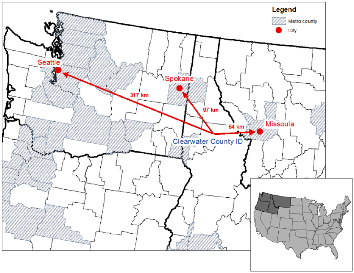
Example of Distance Calculation
For the metropolitan sample, incremental distances are measured similarly, except that the distance to the nearest urban area is measured from the population-weighted centroid of the county to the population-weighted centroid of its own MSA, accounting for the notion that more distant counties in an MSA are often growing faster with more land availability. All distances are measured as straight-line distances because spillovers that are important for economic activity are likely to occur via numerous channels, such as travel time, job networks, and public service delivery, which are highly correlated with distance. An alternative intuitive measure, travel time, is not likely to offer sizable improvement over our operationalization as road travel time can be affected by time of day with rush hour, for example, which would introduce a measurement error that would be more systematically severe in large metropolitan areas and potentially may bias our results. If our choice of an approximation introduces some measurement error, the only tangible effect would be that distance coefficients are biased to zero and the standard errors would be measured less precisely (see Partridge et al. 2008), 11 so our results represent conservative estimates. Because the first-difference approach removes all time-invariant county-specific fixed-effects, including proximity or remoteness from urban centers, the estimated distance coefficients show how the effects of urban hierarchy accessibility are changing over time—for example, a significant positive coefficient would suggest that the role of distance in helping more remote areas to grow (for example, by “insulating” from urban competition) is increasing over time.
In addition to the explanatory variables described above, the vector
Summary Statistics for the Variable by Sample

NOTE: The table reports means that are not weighted by population.
Estimation Results and Discussion
This section presents estimation results for both self-employment and wage and salary employment discussed below separately for the metro and nonmetro subsamples. Since the dependent variables, industry mix term, and employment growth in nearby MSAs are calculated relative to total county employment, estimation coefficients on the main explanatory variables in each model are directly comparable. One should keep in mind that the industry mix variable is calculated using total employment that includes both self-employment and wage and salary employment, whereas the dependent variables separate these two employment groups. To meaningfully interpret the industry mix coefficients in Tables 3 and 4, we need to adjust for the share of self-employed (reported in Table 2) in the four subsamples that we analyze.
Shares of Nonagricultural Self-Employment in Four Groups of Counties

SOURCE: Authors’ calculations based on the EMSI data.
Nonmetropolitan sample results
In this subsection, we discuss results for the nonmetro subsample broken down into rural and micropolitan groups. 12 Table 3 reveals clear differences in the effects of self-employment and wage and salary employment growth determinants. For self-employment, the industry mix term has a modest but positive impact on self-employment growth; however, the effect in micropolitan counties is twice as large. The gap is even larger if we account for the average nonfarm share of proprietors in the rural and micropolitan subsamples. Using Table 2, we can interpret the coefficient of 0.12 for rural counties as 0.03 percent spillovers. That is, a 1 percent increase in exogenous employment from having a favorable industry composition increases rural self-employment by 0.12 percent. Because rural self-employment averages 9.3 percent of total employment, this 1 percent of expected increase in total employment on average should consist of 0.09 percent of new self-employed jobs and 0.91 percent of new paid jobs, suggesting that self-employment grows by an additional 0.03 percent above what would be expected if the economic shocks created jobs in the same proportion as the share of self-employment. Likewise, the coefficient of 0.25 in the micropolitan subsample can be interpreted as 0.18 percent spillovers because micropolitan self-employment averages 7 percent of total employment. The spillover is six times larger than the one in the rural subsample, indicating that micropolitan counties on average create more self-employed jobs after a positive economic change.
OLS Estimation Results for Nonmetro Counties

NOTE: Standard errors clustered at 177 BEA economic areas in parentheses.
p < .1. **p < .05. ***p < .01.
Rural self-employment benefits from growth in the nearest small MSA. Every 100 new jobs in such metro areas on average are associated with 4.5 new self-employed jobs in rural surrounding counties, but only 2.7 new jobs in micropolitan surrounding counties, after three years. In addition to enjoying positive spread effects from small MSAs, micropolitan self-employment also benefits from growth in nearby medium-size metros. Micropolitan self-employment is not affected by economic conditions in nearby large MSAs, whereas self-employment growth in rural areas is suppressed if the closest MSA grows and happens to be large. The magnitude of the corresponding coefficients shows that rural backwash effects from nearby large MSAs are almost three times larger than positive spread effects from small MSAs. Insignificant coefficients on the distance-MSA-size-growth interaction terms suggest that distance to a nearby MSA does not affect the magnitude of the estimated MSA growth effects.
Turning directly to the main distance variables, which reflect changes in the effects of proximity over time, the positive and significant distance to the nearest MSA coefficient suggests that greater distance provides proprietor businesses increasing protection from urban competitors. Yet as noted above, some of the adverse urban competition effects are mitigated for growing small and medium MSAs, which is consistent with Partridge et al.’s (2008) findings that medium and small MSAs have larger spillovers. Incremental distance to the nearest metro area of fewer than 250,000 people also offers additional protection, but incremental distances to higher-tier cities are statistically insignificant. This might suggest that backwash is becoming more pronounced in the twenty-first century, which differs from the findings reported by Partridge et al. (2010).
Coefficients on the 1990 control variables tell several stories. First, the magnitude of the coefficients is very small, so that while some are statistically significant, we do not want to overstate their economic consequences. Next, the legacy of agricultural specialization in micropolitan counties appears to be associated with some growing reductions in self-employment. Relatively low levels of educational attainment have (modest) ever-increasing effects in promoting self-employment in both rural and micropolitan counties, whereas greater shares of adults with a graduate or professional degree have a growing impact on self-employment only in the micropolitan subsample. This may point to an increasing prevalence of necessity entrepreneurship in rural areas. In micropolitan counties the results seem to suggest increasing roles for both necessity and opportunity self-employment as follows from the positive and significant coefficients on both educational attainment measures. Larger rural counties, as measured by population in 1990, tend to have decreasing rates of self-employment growth, which is a little surprising unless incorporated businesses are crowding out self-employment, which mostly consists of partnerships and not limited liability corporations.
We now briefly describe the wage and salary results shown in the right panel of Table 3. They suggest that the dynamics behind nonmetro paid employment is different from that behind self-employment. In particular, a 1 percent exogenous change in employment due to local industry composition is associated with 1.8 percent more rural wage and salary employment (significant at the 5 percent level) but leads to a statistically insignificant 1.1 percent increase in micropolitan paid employment. One implication is that in sparsely populated rural counties, favorable economic changes have, on average, larger impacts.
The spread effects from the nearby small and medium MSAs are consistent with the self-employment results. The only difference is that growth-spread effects from small MSAs are stronger in micropolitan counties. No backwash effects are detected for wage and salary employment. Likewise, distance to nearest MSA of any size is statistically unrelated to wage and salary employment growth. In rural counties, two distance-growth interaction terms are significant. Although the lack of statistical significance of the main effects complicates interpretation, one may conclude that the protective effect of distance from growing medium MSAs is greater if they grow faster, whereas protective effects of distance from large MSAs is decreasing when these large metro areas experience faster growth. Incremental distance to the nearest medium MSA has a growing negative effect on rural paid employment growth, indicating greater job creation closer to such urban centers. This may be due to greater access to markets and suppliers, which promotes wage and salary employment. In the micropolitan subsample, to the contrary, incremental distance to urban centers of 250,000–499,999 residents in 1990 offers additional protection from urban backwash effects. Overall, the results for variables that measure distances seem to point to the changing presence of both spread and backwash effects of varying intensity, making it hard to draw firm conclusions.
Metro sample results
Table 4 presents the results for counties in small and medium MSAs. The table shows a wide variation in the effects of the main explanatory variables depending on employment type and the county’s position in the urban hierarchy. With approximately equal 6 percent self-employment shares in small and medium metropolitan counties (from Table 2), economic growth driven by a favorable industry composition has stronger stimulating effects on self-employment in small MSAs—that is, after subtracting 0.06 from the respective industry mix coefficients, there are 0.28 percent spillovers in small as opposed to 0.14 in medium MSAs, showing considerably greater self-employment growth than the expected growth based on its average 6 percent (0.06) share. Job growth in nearby large metro areas and distance to these areas do not affect self-employment in lower-tier MSAs, although there is evidence that possible distance protection is weaker if nearby large MSA growth is greater. Both education variables are positive and statistically significant, again in line with the necessity and opportunity entrepreneurship perspectives.
OLS Estimation Results for Metro Counties

NOTE: Standard errors clustered at 164 BEA economic areas in parentheses.
p < .1. **p < .05. ***p < .01.
In the wage and salary employment models, the industry mix term has differing effects in small and medium metro areas. In small MSAs, industry composition effects suggest that an exogenous 1 percent increase in total employment leads to only an 0.82 percent increase in wage and salary employment, which means that the growth displaces other paid employment. In medium MSAs, the corresponding 1 percent change is associated with 2.5 percent more wage and salary jobs, suggesting high positive multiplier or spillover effects. Growth in MSAs of at least 1.5 million people appears to have strong positive effects on both small and medium MSA paid employment growth, which is more pronounced in medium MSAs.
The direct effect of distance from the own-MSA core (distance to the nearest MSA) is statistically insignificant. For smaller MSAs, the negative and significant incremental distance to MSAs greater than 500,000 and greater than 1.5 million people suggests that the effects of remoteness are declining in smaller cities. In other words, being closer to larger MSAs has increasing importance. The results are similar for medium MSAs, though the incremental distance to MSAs of at least 1.5 million people is insignificant. Both results are consistent with growing spread effects from bigger cities to smaller cities because being closer to larger MSAs is positively related to paid employment growth.
Before we summarize our main findings in the next section, it is important to note that this study documents the differences in the effects of national economic conditions and of employment growth in nearby MSAs on local self-employment and paid employment as a function of a locality’s position in the rural-urban hierarchy and of the size of a nearby MSA. Our research design ensures that we detect a statistically strong relationship since the main explanatory variables in the models are predominantly significant even after differencing and a use of instrument-like measures. Our research design, however, does not allow us to draw detailed conclusions on the specific mechanisms that lead to the documented differences. We, thus, rely on previous literature in our attempt to explain the phenomena that we present and welcome future research that would formally test potential explanations.
Conclusion
Since Birch’s (1979) work on the importance of small businesses, economists and policy-makers have championed them as key economic drivers. At the same time, scholars are increasingly aware that entrepreneurship is not fostered inside a vacuum and that key environmental factors influence the probability of initial success and maturation of start-ups. Our study contributes to this discussion by investigating the relative local job growth effects from exogenous economic changes on self-employment and paid employment. We also investigate how these relationships change according to the locality’s position within the urban-rural hierarchy.
Our analysis arrives at three important conclusions. First, we demonstrate that the response of local self-employment to exogenous economic shocks varies by the local county’s position in the urban-rural hierarchy. Overall, self-employment in rural counties is the least responsive to such exogenous changes. In rural counties with higher shares of workers who have only a high school diploma, rising rates of self-employment may indicate the prevalence of “necessity entrepreneurship.” Whether the emergence of necessity entrepreneurship is a drag on local growth is debatable—the answer likely varies across the urban hierarchy; however, the distinction between necessity and opportunity entrepreneurship often used in the literature (Low, Henderson, and Weiler 2005) may be a misnomer, especially in lagging and remote regions (Stephens and Partridge 2011).
Second, we document the presence of both spread and backwash effects. Most likely, these effects work simultaneously via various channels whose intensities depend on a number of factors. This article explores the role of two such factors—a position within the urban-rural hierarchy and a nearby MSA size—that indeed appear to play a role in what effect dominates. Overall, backwash effects are evident in the influence of large metro employment growth on self-employment growth in surrounding rural counties. In all other cases, either spread effects are predominant or no effects are detectable, most likely because of their offsetting impacts.
Finally, depending on the relative positions of counties within the urban-rural hierarchy and the type of employment considered, distance to nearby MSAs plays both protective (allowing faster self-employment growth in more remote nonmetro counties) and stimulating (promoting growth in counties closer to urban centers, in line with the view that access to markets and resources are important) roles, although the empirical evidence on the presence of the latter is weaker. While distance is not something that can be directly affected by policy levers, local decision-makers should exploit any advantages and realize limitations that their jurisdictions may face that stem from the jurisdiction’s position on the urban-rural continuum. Future research may examine how exogenous changes in economic growth affect other outcomes such as income, poverty, and inequality to help to better tailor policy design within the urban-rural hierarchy.
Footnotes
Appendix
Industry mix variable is calculated as described in equation (A1). To keep our specification consistent, we difference the industry mix term over three years.
where subscripts c, t, and τ indicate county, time period, and a year within time period t, respectively; and subscript i refers to an industry. For each industry (at the four-digit NAICS level) within a county, we calculate the share of total county employment in the beginning of a three-year period (
NOTE:
We appreciate the partial support of USDA AFRI grant #11400612, “Maximizing the Gains of Old and New Energy Development for America’s Rural Communities.”
Notes
Alexandra Tsvetkova is a postdoctoral researcher at The Ohio State University, Department of AED Economics. Her research on regional economic performance determinants has appeared in Energy Economics, Small Business Economics, Regional Science and Urban Economics, Economic Development Quarterly, and other journals.
Mark Partridge is the C. William Swank Chair of Rural-Urban Policy at The Ohio State University and a professor in the Department of AED Economics. He is also an adjunct professor at Jinan University, Guangzhou, China, and at Gran Sasso Science Institute, L’Aquila, Italy. He has published in journals such as the American Economic Review, Journal of Economic Geography, Journal of International Economics, Journal of Urban Economics, Journal of Business and Economic Statistics, and Review of Economics and Statistics.
Michael Betz is an assistant professor in the Department of Human Sciences at The Ohio State University. His research explores factors that drive local labor markets and demographic change in the United States, with a particular focus on differences between rural and urban areas. He has published in the American Journal of Agricultural Economics, Energy Economics, Papers in Regional Science, Rural Sociology, and International Regional Science Review.
References
Supplementary Material
Please find the following supplemental material available below.
For Open Access articles published under a Creative Commons License, all supplemental material carries the same license as the article it is associated with.
For non-Open Access articles published, all supplemental material carries a non-exclusive license, and permission requests for re-use of supplemental material or any part of supplemental material shall be sent directly to the copyright owner as specified in the copyright notice associated with the article.
