
Abstract
In this article, I propose a three-stage estimation model to examine the effect of parental divorce on the development of children’s cognitive skills and noncognitive traits. Using a framework that includes pre-, in-, and post-divorce time periods, I disentangle the complex factors affecting children of divorce. I use the Early Childhood Longitudinal Study-Kindergarten Class 1998 to 1999 (ECLS-K), a multiwave longitudinal dataset, to assess the three-stage model. To evaluate the parameters of interest more rigorously, I employ a stage-specific ordinary least squares (OLS) model, a counterfactual matching estimator, and a piece-wise growth curve model. Within some combinations of developmental domains and stages, in particular from the in-divorce stage onward, I find negative effects of divorce even after accounting for selection factors that influence children’s skills and traits at or before the beginning of the dissolution process. These negative outcomes do not appear to intensify or abate in the ensuing study period.
A majority of studies in the literature on divorce find adverse effects of parental divorce 1 on children’s development (Amato and Keith 1991; Cherlin, Chase-Lansdale, and McRae 1998; Hetherington 2003; Wallerstein and Lewis 2004). Two authoritative meta-analyses show that, compared to children with continuously married biological parents, children with divorced parents are disadvantaged regarding various life outcomes, including likelihood of dropping out of high school, cognitive skills, psychosocial well-being, and social relations (Amato 2001; Amato and Keith 1991). Traditional ordinary least squares (OLS) frameworks, as well as more recent statistical techniques such as propensity score matching and behavioral genetics, confirm the negative effects of divorce. 2 Moreover, research shows that these negative consequences have not diminished even as the social stigma attached to divorce has declined significantly (Amato 2001; Sigle-Rushton, Hobcraft, and Kiernan 2005).
A more recent strand of research, however, questions the traditional hypothesis of homogenous negative outcomes and the empirical evidence used to support this hypothesis. Among the many empirical and theoretical challenges, scholars note the possibility of selection bias; the need to further investigate observations of remarkable resilience among subpopulations; and the need for more nuanced approaches to separate the genuine effects of divorce from possibly confounded effects related to other family processes that precede or follow divorce, such as marital discord and remarriage (Amato and Booth 1997; Cherlin et al. 1991; Hetherington 1979; Kelly and Emery 2003). For example, partly due to the absence of appropriate data, research has not explicitly addressed whether prior marital conflict between parents is primarily responsible for children’s outcomes or whether there are distinctive effects of the dissolution process (Amato, Loomis, and Booth 1995; Hanson 1999). Furthermore, it remains to be seen whether children of divorce successfully catch up with their counterparts or whether these children experience further developmental setbacks after divorce (Hetherington 2003; Wallerstein and Lewis 2004).
To date, scholars have conducted few rigorous studies incorporating these complex features (for exceptions, see Allison and Furstenberg 1989; Cherlin et al. 1991; Sun and Li 2001). To fill this gap in the literature, I employ a three-stage model of the effects of divorce on child development to examine the distinct and combined effects during the pre-divorce, in-divorce, and post-divorce periods. I hasten to add that this is not the first project to examine differences in developmental outcomes across divorce stages. For instance, Sun and Li (2002) assess differences in various cognitive and noncognitive outcomes in four stages (at ±3 and ±1 years of divorce; see also Aughinbaugh et al. 2005).
I am unaware, however, of any previous studies that attempt to (1) formulate stage-specific hypotheses, such as a marital conflict hypothesis in the pre-divorce stage and a resilience hypothesis in the post-divorce stage, (2) evaluate hypotheses in a manner rigorous enough to estimate stage-specific effect parameters, and (3) provide a unified framework by integrating stage-specific effects within the rubric of total divorce effects. My three-stage model is designed to overcome the limitations of previous studies while utilizing the basic idea, introduced by other scholars, of conceiving of divorce as a process (Hetherington 1979; Morrison and Cherlin 1995). In addition, the three-stage model enables me to disentangle complicated issues of causal inference that most previous studies fail to recognize. For instance, as I will discuss in detail, scholars often control for concurrently measured covariates to obtain post-divorce effect estimates, which leads to potentially biased estimates (Rosenbaum 2002).
To attain these goals, I examine data from the Early Childhood Longitudinal Study-Kindergarten Class 1998 to 1999 (ECLS-K) (Tourangeau et al. 2006), which followed children from kindergarten through 8th grade and measured a rich set of family background variables. ECLS-K provides a prime opportunity to assess several competing hypotheses concerning causal inferences about the effects of divorce. From a methodological perspective, a traditional OLS regression framework is limited. In particular, this approach assumes a balanced covariate set between children of divorce and children from intact families. This assumption is quite burdensome for the current study, however, because my very strict definition of divorce means the sample contains few observations of children of divorce.
Given the large number of children from intact families (n = 3,443) and the relatively small number of children of divorce (n = 142), a matching estimator is the recommended statistical technique for obtaining parameters of primary interest (Rosenbaum and Rubin 1983; Smith 1997). In addition, the estimate of interest, the average treatment effect on the treated (ATT), provides a more appropriate and attractive interpretation. ATT estimates the average difference between the realized developmental outcomes for children of divorce and the counterfactual outcomes for these children had their parents remained married (Heckman, Ichimura, and Todd 1998; Heckman and Navarro-Lozano 2004). OLS and matching estimators appear inadequate, however, in the face of multiwave longitudinal data because one cannot draw statistical inferences on stage-intersecting parameters, such as total divorce effects (Raudenbush and Bryk 2002; Singer and Willett 2003). To overcome this shortcoming, I supplement stage-specific and combined OLS and matching estimates with estimates from piece-wise growth curve models.
Conceptual Frameworks
To facilitate the theoretical discussion, Figure 1 schematizes hypothetical developmental trajectories for children of divorce and children with continuously married biological parents. The x-axis refers to the time frame and the y-axis refers to developmental outcomes (e.g., math test scores; higher indicates a better score). The index T refers to observation time points and D denotes divorce, which occurs between T2 and T3 .
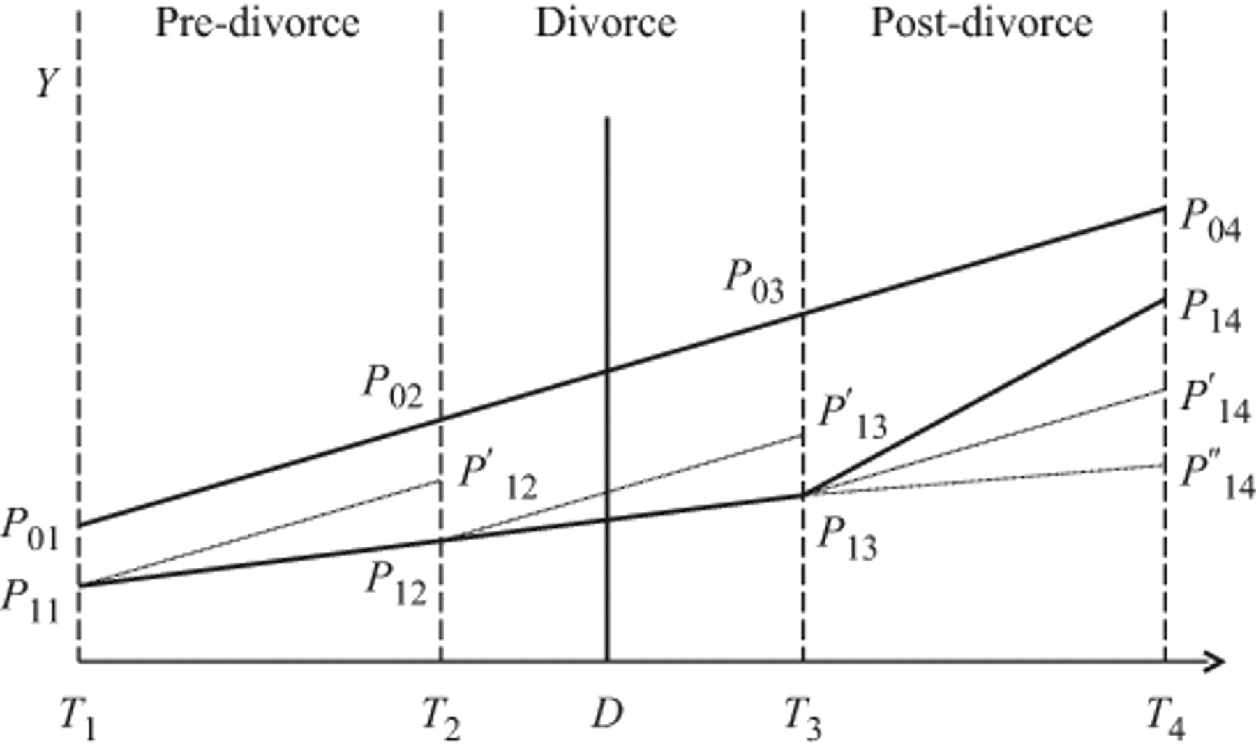
Hypothetical Trajectories of Developmental Outcomes
In Figure 1, the developmental trajectory of children in intact families is hypothesized to move along the upper solid line: P 01 → P 02 → P 03 → P 04. By contrast, outcomes for children of divorce are hypothesized to follow the lower solid line: P 11 → P 12 → P 13 → P 14. The latter trajectory reflects a theoretical position that accounts for selection bias and measurement error in locating the exact time that marital discord surfaced. As Figure 1 illustrates, I hypothesize a negative pre-divorce effect and an unfavorable in-divorce effect, but measurable resilience in the post-divorce period.
Some selection variables operate in a negative manner. For instance, children’s negative psychological predispositions or frailties may be related to an elevated risk of parental divorce (Cui, Donnellan, and Conger 2007) and delayed developmental outcomes before, during, and after parents’ marital conflict materializes (Amato 2001; Cherlin et al. 1991). Positive selection effects may also exist; parents who are more caring and responsive toward their loved ones might be more likely to stay married (Sun and Li 2001). If these selection mechanisms are not addressed when estimating differential growth in subsequent stages, results will attribute an unwarranted portion of selection effects to the incidence of divorce. However, I do not focus on the initial gap between P 01 and P 11, which may be generated by selection mechanisms, because I am interested in differential growth in subsequent stages and including lagged outcome variables in the models will adjust for previously generated gaps.
Determining the exact date at which family dysfunction or parental conflict owing to marital discord emerged is another potential source of measurement error (Morrison and Cherlin 1995). If marital discord predates T 1 and adversely affects children, measurement error would result in children’s initial development level being estimated at a point below P 01, such as P 11. In this case, failing to account for the negative outcome by conditioning on T 1 would understate the overall negative effects attributable to events in the pre-divorce phase. Conversely, if marital discord emerges after T 1, such a bias would not occur. Given that the empirical data have a one-year interval between T 1 and T 2, the former scenario seems more likely.
Scholars of divorce generally agree that marriages that end in divorce are plagued by dysfunction and conflict before the formal separation process begins, thus exposing children to the risk of developmental setbacks (Amato and Booth 1997; Cherlin 2008). This notion of a negative pre-divorce effect is based on two premises: intense marital conflicts and their negative influence on children’s development. Some recent research suggests the possibility of reverse-causation of child effects on marital conflicts (e.g., Cui et al. 2007; Jenkins et al. 2005), but most evidence supports the former premise (Hetherington 1979; Peterson and Zill 1986). In reviewing the developmental psychology literature, for instance, Emery (1982:312) concludes that “although methodology can affect estimates of the magnitude of the relation between marital and child problems, the relation is nevertheless a real and important one.”
Yet the premise that parents destined to divorce are discernible by intense marital conflicts is not well-established and has been challenged. For example, Amato (2002) characterizes a sizable number of divorces as “good enough marriages” in which marital discord is not readily noticeable. In a similar vein, using the National Survey of Families and Households (NSFH), Hanson (1999) finds that only about 50 percent of divorced couples engaged in a high level of marital conflict. Furthermore, Hanson shows that 75 percent of couples in the high conflict category decided not to divorce, suggesting that children with intact families also experience parental marital discord. Nevertheless, I hypothesize a negative pre-divorce effect, on average, because “good enough marriages” destined to divorce have relatively low marital quality, and conflict-ridden marriages that result in divorce exhibit more intense conflict.
Figure 1 also illustrates control-away bias if I fail to consider the pre-divorce process, given the assumption of noticeable pre-divorce conflicts and their negative consequences. Namely, if one estimates divorce effects using measurements from T 2 as baseline control variables, as most researchers do, analyses would underestimate the total negative effects of divorce because the already-present marital conflicts would decrease positive outcomes in T 2, artificially diminishing unfavorable developments tracing back to T 1. Controlling for T 2 outcomes is valid, however, when considering the in-divorce effect, defined as the difference in developmental growth in the period spanning from T 2 to T 3.
As discussed earlier, ample evidence supports the concept of relatively deteriorating outcomes for children of divorce in the divorce stage (Amato 1993; Lansford 2009). Many theoretical mechanisms can account for this pattern, including continuing conflicts between separating parents (Emery 1982; Hetherington 1979), emotional troubles or a lack of resources from divorced parents when adjusting to a new environment (Cooper et al. 2009), economic hardship due to a sudden drop in family income (McLanahan and Sandefur 1994; Morrison and Cherlin 1995; Peterson 1996), and geographic relocation and school transfer following divorce (Astone and McLanahan 1994).
Such evidence notwithstanding, the possibility of routes through which parental divorce might contribute positively to a child’s well-being cannot be excluded. Most notably, one research question in the literature asks whether children of divorce are better off after parental divorce if they were exposed to a high level of parental conflict. In their classic work, Amato and colleagues (1995) assess this hypothesis with respect to children’s psychological well-being and overall happiness and find that children who endured high marital conflict and divorce report more positive outcomes than do children who experienced high marital conflict but no divorce (for more reserved findings, see Hanson [1999]). Recent work by Aughinbaugh and colleagues (2005) also challenges the traditional notion of homogeneous negative in-divorce effects; based on maximization of total utility among involved parties, they suggest possible benefits for children of divorce. Thus, I do not discard the possibility that the developmental trajectory for children of divorce might move along P 12 → P′13 instead of P 12 → P 13.
Figure 1 also illustrates an assumption of measurable resilience after divorce, via P 13 → P 14 (Hetherington 2003; Kelly and Emery 2003). It is important to be clear about the meaning of “resilience,” a controversial concept with multiple meanings. First, there is no unified definition. Indeed, there is ambiguity regarding (1) which personal or family characteristics lead to resilience, (2) whether resilience should refer to bouncing back from previous adverse outcomes or to the relative absence of vulnerability to risk exposure, and (3) how to measure resilience (Kaplan 2005). In the current context, should I describe resilience as occurring among children of divorce if I fail to detect negative pre-, in-, or post-divorce effects, because divorce has an adverse impact but children presumably overcome the risk? Doing so would extend the concept of resilience too far, because this misses the point that one should not assume divorce effects are negative. I thus define resilience as bouncing back from previously negative outcomes, illustrated by P 13 → P 14.
This definition of resilience is not necessarily confined to the post-divorce period. In an extreme case, resilience may be present when there are noticeable negative outcomes in the pre-divorce period but significant positive turn-around occurs during the in-divorce period. This theoretical possibility does not occur in my analyses, however, so I restrict resilience to the post-divorce period. By contrast, if the developmental growth of children of divorce kept pace with that of children from intact families, then the former children would follow the path P 13 → P′14 (which is parallel to P 03 → P 04). In this case, I would not describe these children as resilient. Antithetical to the resilience argument, children might follow P 13 → P″14 if there are significant negative effects after divorce (Cherlin et al. 1998; Wallerstein and Lewis 2004). If detrimental mechanisms present during the in-divorce period continue into the post-divorce period, I would observe a widening gap in developmental outcomes.
In this regard, scholars have devoted much attention to family formation and its distinct effects on children’s post-divorce development, because new family formation is a confounding factor when identifying effects inherent to divorce. Evidence is mixed, however, as to whether new family formation has aggregate negative effects. Using the Fragile Family and Child Wellbeing Study, for instance, Cooper and colleagues (2009) find that family transition type and number of transitions are related to parental stress. By contrast, Thomson and colleagues (2001) find that mothering behaviors and mother-child relationships improve when mothers remarry or enter partnerships, although the amount of elapsed time might affect the results. One recent article analyzing the Children of the National Longitudinal Study of Youth (CNLSY) 1979 concludes that, among white children, some noticeable differences in outcomes occur dependent on a number of family structure transitions: differences in cognitive achievement nearly disappear, while a somewhat strong relationship remains significant for externalizing behavior problems, even after introducing a rich set of selection factors (Fomby and Cherlin 2007).
Statistical Strategies
Because I use multistage estimation strategies, typical OLS regression is ill-suited for this study. To develop more cogent statistical models, let me refer to Y
t
as a developmental outcome measured at time t ∈ {0,1,2,3,4}. Following conventional notational practice, uppercase letters denote variables and lowercase letters denote realized values. Likewise,
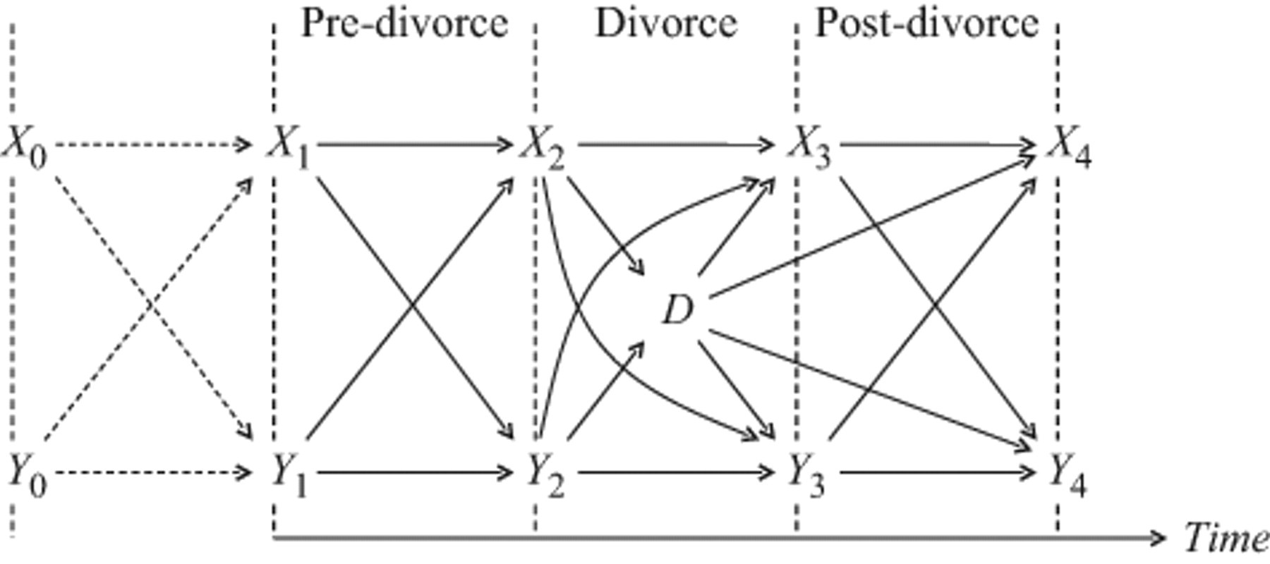
Causal Diagram
When estimating the in-divorce effect, I condition on the covariate set
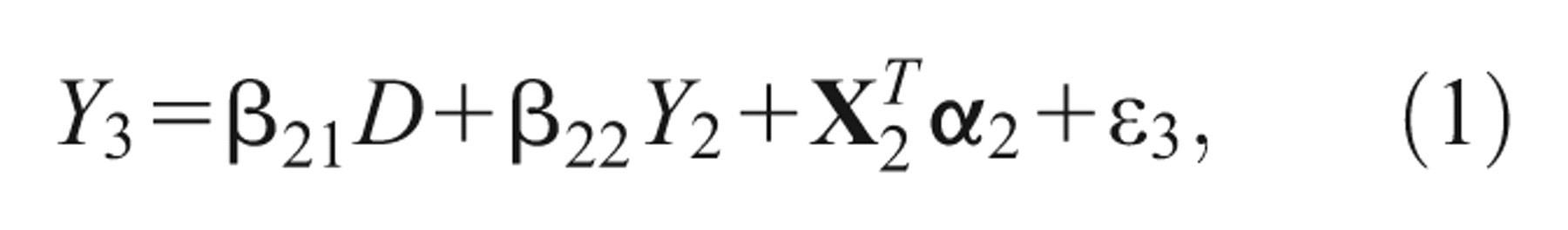
where ε3 represents the error term. As usual, the superscript T (for
Estimating the exact pre-divorce effect is impossible because doing so would entail using D to predict Y 2, even though the former is generated by the latter, a sheer contradiction. This statistically nonsensical enterprise, however, lies on theoretically justifiable grounds. As discussed earlier, most divorces are characterized by marital strain and interpersonal conflict that affect children; therefore, omitting the pre-divorce process would bias total divorce effects in a positive direction. However, it is also crucial to adjust for other covariates that confound the pre-divorce effect. I therefore estimate the pre-divorce effect with the following equation:
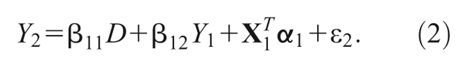
The estimate β11 does not possess any causal meaning, unlike estimates in other stages. Rather, the estimate provides, at best, descriptive conjecture of the pre-divorce effect.
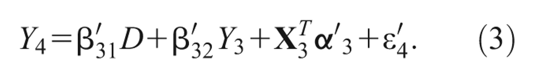
Finally, how can one plausibly determine the post-divorce effect? One possibility is to use Equation 3 and assume β′31 is a relevant estimate:
This approach, however, controls away possible contributions of divorce to the post-divorce effect. Figure 2 shows that, for instance, there is a path from D to Y
4 via Y
3; therefore, controlling for Y
3 blocks this path and leads to bias. Conditioning on Y
3 and
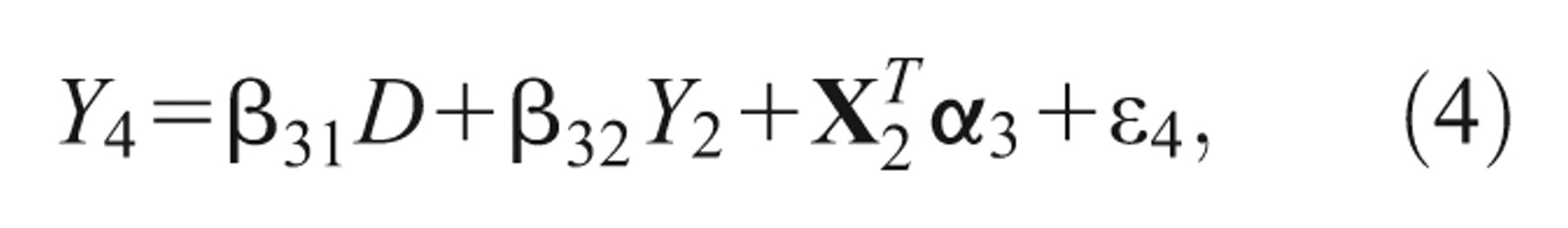
in which β31 represents a combination of in- and post-divorce effects. To obtain the post-divorce effect, I subtract the in-divorce effect from the combined effects (β31 – β21), derived from Equations 4 and 1, respectively. Similarly, I can summarize total divorce effects by adding the pre-divorce effect to the combined effects (β31 + β11). Despite its limitations, I argue that Equation 3 provides useful estimates, particularly in a policy context. Given that predicting parental divorce is a speculative exercise, one can observe children of divorce only after the experience. Policymakers, however, are interested in how much the effects of divorce endure, conditional on currently observed covariates. Equation 3 supplies an answer to this question.
One of the problems of applying an OLS estimator separately to Equations 1 through 4 is that, even though I can obtain point estimates and p-values for stage-specific parameters, the method does not allow for statistical inference of aggregate estimates, such as total divorce effects. The most straightforward way to overcome this shortcoming is to bootstrap subsamples with replacement (Efron and Tibshirani 1993; Lohr 1999). I randomly subsample the analytic data 90 times to maintain consistency with the weighting methods employed to account for longitudinal attrition, as I discuss shortly.
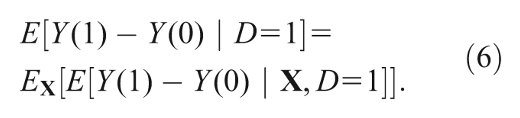
I also use a counterfactual method via a matching estimator because of its ease of estimation and its attractive interpretation, as discussed in detail earlier (Rosenbaum and Rubin 1983; Smith 1997). To develop a formal statistical specification, let Y = Y(0), a potential outcome if a child lived with continuously married parents, and Y = Y(1), the potential outcome when the same child endured parental divorce.
3
Under the assumption of the non-confounded treatment assignment conditional on a set of the observed confounding variables

ATT can be obtained by the iterated expectation formula (Heckman et al. 1998):
Before further discussion, it is worth repeating that unobserved confounding variables pose a serious threat to estimates and inferences using the general class of matching methods.
Currently available matching estimators based on propensity scores do not necessarily provide unbiased estimates if matching is not exact across all covariate values (Abadie and Imbens 2006). Owing to this potential problem, scholars have devoted considerable effort to attaining reasonable balancing in values of covariates among matched pairs (Dehejia and Wahba 2002). Based on this research, I use the “GenMatch” routine in R developed by Sekhon (Diamond and Sekhon 2006; Sekhon forthcoming). Instead of using propensity scores, the genetic matching algorithm stochastically determines a weight matrix minimizing the Mahalanobis distance among confounding variables to achieve tighter balancing. I matched up to six children from intact families to each child of divorce but, as expected, balancing statistics severely deteriorated beyond a one-to-one match. I thus report results using a one-to-one match (see Part B in the online supplement for balancing qualities of covariate values by the number of intact-family children matched to each child of divorce). I also report consistent estimates for the large sample variance developed by Abadie and Imbens (2006), which is a built-in feature of GenMatch.
To estimate the in-divorce effect, I condition observed values of confounding variables at T 2 to match children of divorce with intact-family children and compute ATT. Balancing requirements for matching estimators mean that in a matched sample for the in-divorce effect, values of confounding variables should not differ between two groups of children. Therefore, lagged outcomes included as covariates should not differ, leading to an estimate of zero for the pre-divorce effect when using the matched sample. I thus include confounding variables collected at T 1 and capture the pre-divorce effect using the generated matched sample. This procedure again highlights why estimates of the pre-divorce effect do not possess causal meaning. Regarding estimation of the post-divorce effect, I follow the reasoning outlined earlier.
The final model-building strategy is based on a piece-wise growth curve model. As Figure 1 suggests, the current research problem can be viewed as estimating two different growth trajectories, depending on parental divorce. In addition, the growth curve approach should ameliorate correlation problems within individual levels across time points. I use the “PROC MIXED” routine in SAS for model estimation (Singer and Willet 2003). I encountered convergence problems in several models, even after experimenting with a comprehensive set of initial values. With the hope of normalization, I also tried a log transformation of the noncognitive trait variables on the original metric but found no significant gain. I thus report only the results from the original metrics.
In addition to other methodological challenges, adjusting for longitudinal attrition is a major concern, especially because I delete observations with at least one missing value on all variables in the analyses (list-wise deletion approach). To ameliorate attrition bias, I adopt the design-based method of weighting by a longitudinal weight (“c1_6fp0”) furnished by the data collector (Lohr 1999; Tourangeau et al. 2006). To allow for statistical inference using estimates on weighted data, I follow the recommendation of Tourangeau and colleagues (2006) and employ the “paired Jackknife” method using 90 replicate weights, which takes complex survey design into account. For a more complete report, I show unweighted and weighted estimates.
Data and Measurement
Data
To implement the conceptual and statistical models, I use the ECLS-K longitudinal dataset collected and maintained by the National Center for Education Statistics (NCES). The ECLS-K is a nationally representative study with a multistage probability sample from the population of the 1998 to 1999 kindergarten cohort (Tourangeau et al. 2006). Geographic areas were the primary sampling units, and NCES chose schools as the second-stage units from which students were sampled. The study consists of an initial survey in the fall of kindergarten (1998) and six follow-up waves (the spring of kindergarten [1999], the fall and spring of 1st grade [1999 to 2000], the spring of 3rd grade [2002], the spring of 5th grade [2004], and the spring of 8th grade [2007]).
I do not include the 1st grade fall survey because only a subsample of 30 percent of eligible children completed interviews. Thus, the only children with data before and after divorce are those whose parents divorced between the spring of kindergarten and the spring of 3rd grade. 4 I chose the interview conducted in the spring of kindergarten as the T = 1 survey. Three considerations influenced this decision: (1) test scores in the fall semester may be dominated by summer schooling parameters, (2) teacher-assessed noncognitive traits are more prone to measurement error because of the short observation time, and (3) covariates measured in the fall of kindergarten are needed to construct a reasonable piece-wise growth curve model. In summary, I focus on five surveys: the fall and spring of kindergarten, and the springs of 1st, 3rd, and 5th grades. These survey rounds are denoted by Tt : t ∈ {0,1,2,3,4}, respectively.
Measures
Explanatory variable
I focus on the comparison between children who experienced parental divorce in the period between spring of 1st grade and spring of 3rd grade and children whose parents stayed married throughout that period. I ignore marital status after the 3rd grade interview, so “children of divorce” includes children exposed to further family changes such as cohabitation or remarriage after divorce, as well as children who experienced no other family transitions. Furthermore, I only include children living with two biological parents; children with adoptive parents or remarried parents are excluded from the sample. Only children whose parents’ marriage remained intact from the initial survey until the spring of 1st grade were eligible for the sample. To pursue a more rigorous evaluation of the effects of divorce, I exclude children with a widowed parent at T 3 from the sample (Emery 1982). This rigorous definition of “children of divorce” may equalize the support of covariates between the two comparison groups and, hopefully, ameliorate selection bias in exchange for a reduced sample size.
To avoid confounding divorce effects with effects due to family processes after divorce (e.g., remarriage), it might be helpful to compare children whose divorced resident father or mother remains unmarried or unpartnered with children from intact families. This approach, however, invites more complications by introducing endogenous selection bias (i.e., Berkson’s paradox or explaining-away bias [Elwert and Winship 2008; Pearl 2000]). Endogenous selection bias occurs when one estimates a relationship between an explanatory variable (e.g., divorce) and a response variable (e.g., outcome at T 3) after controlling for a third variable (e.g., subsequent marital status at T 4) that is causally affected by the explanatory and response variables. 5 In addition, the small sample size does not allow for such a detailed analysis.
Response variables
Indexing the development of cognitive skills is a critical issue for the measurement of outcome variables. Test score metrics pose a particular challenge: among the five metrics provided by the ECLS-K public data, the recommendation is to use proficiency probability scores for longitudinal cognitive development analyses (Tourangeau et al. 2006). However, these scores contain nine dimensions for each subject, making implementation quite difficult. I thus use the Item Response Test (IRT) scale scores for this study. The IRT scale score can be interpreted as a probabilistic score with respect to the number of correct answers students would have given if they had answered all 153 questions in math and all 186 questions in reading.
For noncognitive trait measures, I use three teacher-assessed social rating scales designed to capture children’s socioemotional development. 6 Interpersonal social skills refer to behavior involved in “forming and maintaining friendships, getting along with people who are different, comforting or helping other children, expressing feelings, ideas, and opinions in positive ways, and showing sensitivity to the feelings of others”; externalizing problem behaviors indicate how often a child “argues, fights, gets angry, acts impulsively, disturbs ongoing activities, and talks during quiet study time”; and internalizing problem behaviors assess the frequency of “anxiety, loneliness, low self-esteem, and sadness” (Tourangeau et al. 2006:2–23).
NCES collected five noncognitive measures: (1) approach to learning, (2) self-control, (3) interpersonal social skills, (4) externalizing problem behaviors, and (5) internalizing problem behaviors. These submeasures consist of six, four, five, five, and four items, respectively. The scale for each item ranges from “never (1)” to “very often (4).” Split-half reliability for submeasures reveals a high degree of reliability for all measures, typically exceeding .8 (Tourangeau et al. 2006). Of these five measures, I use only the final three in the analyses. The first two variables are highly correlated with test scores, so little new information can be gained from modeling the variables.
In the spring of 3rd grade, NCES added one item to the original externalizing problem behavior construct. Because I use the mean level across individual items in each submeasure, 7 it is unlikely the added item poses any serious problem for the analyses. All scales are adjusted to range from 0 to 3, with high values denoting a high frequency of the relevant behavior. For example, a high score in interpersonal social skills indicates a student with good skills in interpersonal exchanges, while a high score in externalizing problem behaviors suggests a high frequency of problematic behavior.
Control variables
To control for parent-level selection, I include a measure of whether a mother gave birth when she was a teenager and a measure indicating whether parents were married when the focal child was born. Although these are imperfect measures, given the possibility that the focal child may not be the only child, I include them as the best way to account for teenage childbearing and marital selection problems (Carlson, McLanahan, and England 2004). I also use a measure of mother’s psychological well-being at T 1. NCES collected data on 12 self-assessed items on psychological well-being (e.g., “How often during the past week did you feel depressed?”). Each item ranges from 1 (never) to 4 (most of the time). Alpha reliability of the 12 items is .857 when using total available samples. I calculated the average of the 12 items and subtracted one, to create a range of zero to three, and I use the measure as a control variable with a continuous scale.
I also include a self-assessed measure of global happiness in marital relationships. In the spring semester of kindergarten, the questionnaire asked parents to rate their happiness with their marital relationship. Responses include not too happy, fairly happy, and very happy. Because the variable is highly skewed to the left, I include it as a categorical variable. Socioeconomic status is a critical aspect of the analyses (Cherlin 2008; McLanahan and Sandefur 1994). I use a socioeconomic status index, calculated as the average of five family background variables (i.e., father or father figure’s education and job prestige, mother or mother figure’s education and job prestige, and household income); each variable is normalized to have a mean of zero and one standard deviation before being summed (Tourangeau et al. 2006).
In addition to these variables, I consider the following basic demographic variables: age in months in June 2000 (Emery 1982; Hetherington 1979), gender (Amato and Keith 1991), race/ethnicity (Bulanda and Brown 2007), disability status (Cherlin et al. 1991), number of siblings, urbanicity (Gautier, Svarer, and Teulings 2009), geographic region (Glenn and Shelton 1985), and school moves between two adjacent waves (Astone and McLanahan 1994; Boyle et al. 2008). 8
Results
Descriptive Statistics
Table SC-1 in the online supplement includes descriptive statistics for divorce, outcome, and lagged outcome variables in the analytic sample, with and without longitudinal weights. I provide descriptive statistics separately for the two groups because one estimator employs a matching method to ascertain the average treatment effect on the treated, such that an understanding of children of divorce is essential for evaluation of statistical estimates. Table SC-2 in the online supplement presents descriptive statistics for control variables. Of the total sample of 3,585 children, only about 4 percent (142 children) experienced parental divorce between the spring semester of 1st grade and the spring semester of 3rd grade. When weighted, the estimate increases slightly to over 6 percent, which suggests that, compared with children of continuously married parents, more children of divorce were lost to follow-up by the spring of 5th grade. 9
Regarding cognitive skills, I find that (1) an average difference between the two groups was already present in the initial survey and (2) this difference seems to have increased over time, but (3) it is unclear whether the growing difference provides compelling evidence of a diverging difference because the population standard deviation also increased over time. To illustrate, the average unweighted and weighted sample differences in math test scores was 3.7 and 3.4, respectively, in the fall of kindergarten, and these differences rose to 7.2 and 10.5 by the spring of 5th grade. However, population standard deviations also more than doubled in this period. These findings are consistent in weighted and unweighted samples, although mean estimates of reading scores are consistently moderately lower in the weighted sample than in the unweighted sample.
Results are similar across noncognitive trait measures: there is no patterned increase or decrease in average levels for specific subpopulations. For the internalizing problem behavior variable, however, there is a noticeable increase in the difference between groups in the period from T 2 to T 3, during which parents filed for divorce. Taken together, these findings suggest there may be a strong selection effect beginning at (or, more likely, before) the time of the baseline survey. Furthermore, divorce may not affect entire domains of developmental outcomes, but may influence more specific and selective areas of children’s outcomes.
Table SC-2 in the online supplement reveals differences in some selection-related variables. For example, 14.2 percent of mothers in intact families gave birth as a teenager, in contrast with 34.5 percent of mothers whose parents were divorced. A substantially higher percentage of couples (13.4 percent) in divorced families were not married at the time of the focal child’s birth, compared with the proportion among intact families (6.0 percent), although the difference drops to 8.9 and 6.8 percent, respectively, when the observations are weighted. Furthermore, parents who eventually divorced were more likely to report marital dissatisfaction in the baseline survey and reported a somewhat higher score on psychological symptoms. Socioeconomic variables also vary noticeably. Specifically, in all survey waves, children from intact families enjoyed, on average, a socioeconomic status .3 to .4 points higher than children of divorce. These results are hardly surprising given repeated findings consistent with this pattern (Cherlin 2008; McLanahan and Sandefur 1994).
With regard to other confounding variables, data in Table SC-2 suggest there is no significant difference in the marginal distribution of basic demographic variables such as age and gender, although black children are somewhat overrepresented in the divorced population (Bulanda and Brown 2007). I do see a dramatic change in the distribution of urban location, contingent on whether the sample is weighted. When weighted, more children of divorce reside in cities but there is no distinguishable pattern otherwise. Given previous reports documenting higher divorce rates in urban areas, the weighted estimates seem more reliable (Gautier et al. 2009). The data indicate that children of divorce have an enhanced risk of school moves, particularly around the time of divorce, which may be due to the association between risk of geographic mobility and risk of divorce, regardless of causal precedence (Boyle et al. 2008; Glenn and Shelton 1985).
Statistical Results
Tables 1 through 5 display the statistical results of the analyses. For each outcome variable, I estimate three classes of statistical models: an OLS regression, a matching model, and a piece-wise growth curve. For each model, I fit weighted and unweighted samples. In the unweighted sample estimation, I provide standard errors and their p-values based on asymptotic theory as well as those obtained by the bootstrap method. Model names in the tables are designed to illustrate which phase is associated with which column. For example, T 1 → T 2 means the column contains estimates for outcome variables measured at T 2 with explanatory variables collected at T 1. (T 2 → T 4 ) − (T 2 → T 3 ) is a natural extension of this notation, indicating that I subtracted the estimate T 2 → T 3 from the estimate T 2 → T 4 to lessen control-away bias. In the same vein, I construct total divorce effects by summing three estimates (T 1 → T 2 → T 3 → T 4 ) or by adding two estimates (T 1 → T 2 → T 4 ).
I begin with the results of models predicting math test scores (see Table 1). In general, point estimates suggest lower performance among children of divorce compared to children with continuously married biological parents. Somewhat surprising, however, is that the pre-divorce effect has consistently positive estimates, even though most coefficients do not attain statistical significance. Estimates of the in-divorce effect, while in accord with my theoretical predictions, are statistically insignificant.
Estimates from Statistical Models with Mathematics Test Score as a Response Variable
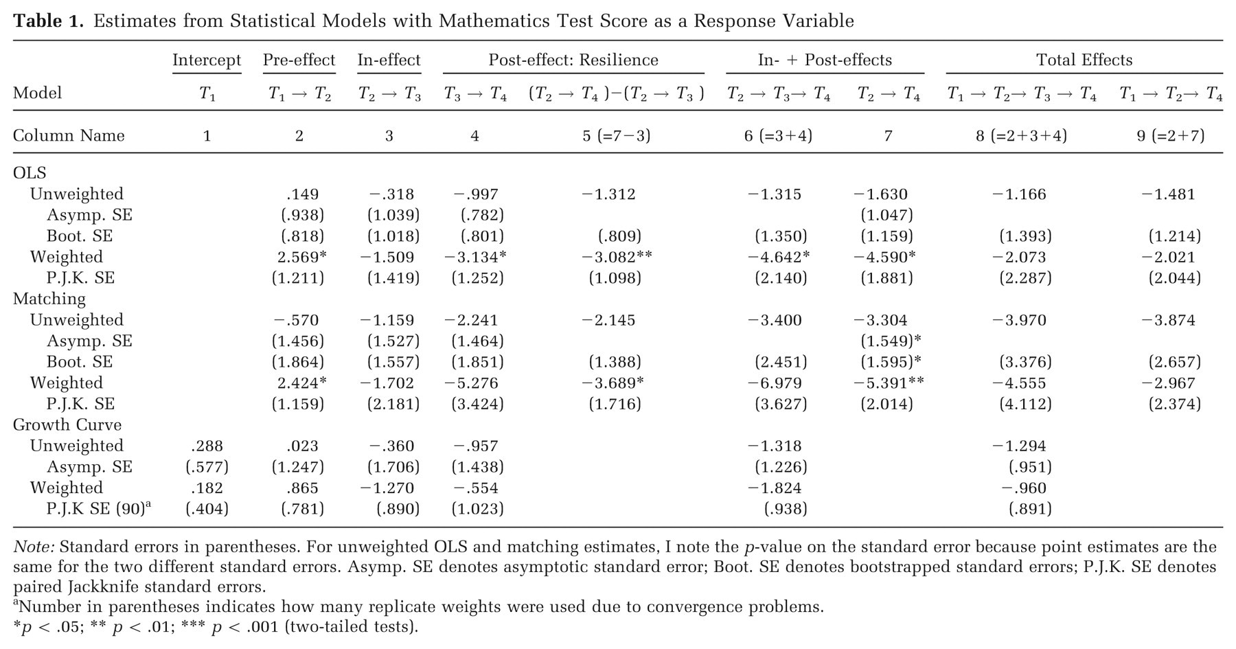
Note: Standard errors in parentheses. For unweighted OLS and matching estimates, I note the p-value on the standard error because point estimates are the same for the two different standard errors. Asymp. SE denotes asymptotic standard error; Boot. SE denotes bootstrapped standard errors; P.J.K. SE denotes paired Jackknife standard errors.
Number in parentheses indicates how many replicate weights were used due to convergence problems.
p < .05; ** p < .01; *** p < .001 (two-tailed tests).
Combined effects of the in- and post-divorce stages are statistically significant, predominantly within the conventional p-value of α = .05, especially when combined effects are defined by T 2 → T 4 and matching estimates are considered (see Cherlin and colleagues [1991] for similar results for a sample of girls; a close look at Sun and Li [2001] reveals similar findings). For instance, math scores for children of divorce were, on average, 5.4 points lower than the counterfactual scores these children would have attained had their parents remained married, when estimated using the combined effects in the framework of path T 2 → T 4 with weights considered. Descriptive statistics indicate that this difference is approximately 30 percent of one standard deviation of T 4. When estimating the effect using T 2 → T 3 → T 4, however, statistical inferences differ across weighting methods. To contextualize these results, the random attrition assumption provides statistically insignificant estimates, while adjusting for attrition indicates a statistically significant difference. Regarding total divorce effects, I see that all estimates are statistically insignificant.
Estimates of reading test scores (see Table 2) align closely with the expected negative in-divorce effects. Yet due to imprecise point estimates, the null hypothesis of the zero effect cannot be rejected (Sun and Li 2001). Unweighted OLS and matching estimates suggest a weak negative in-divorce effect and a combined in- and post-divorce effect (significant at α = .1; not shown in table). Results are too method-sensitive, however, to be accepted without question as a rigorous evaluation of a hotly-debated topic. In particular, because I lean toward estimates from the weighted sample and I am concerned with the regression-to-the-mean weakness of OLS (Smith 1997), I do not conclude that there are significant divorce effects in reading test scores.
Estimates from Statistical Models with Reading Test Score as a Response Variable
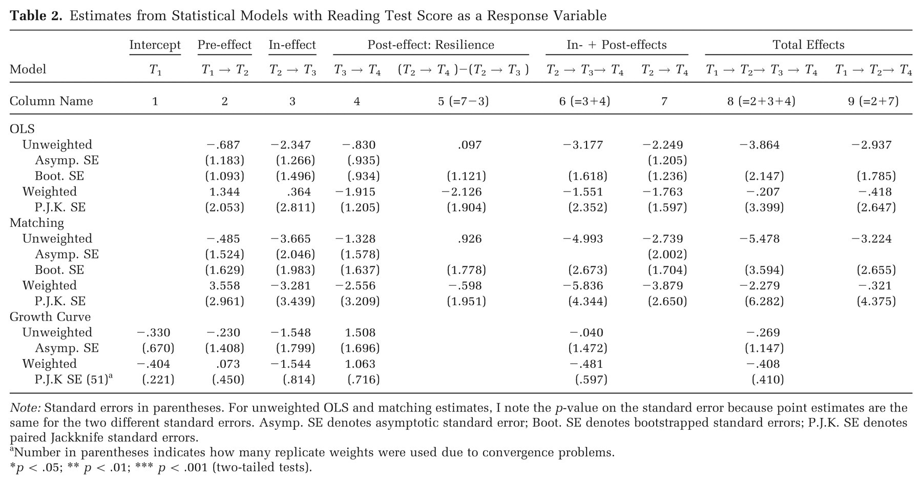
Note: Standard errors in parentheses. For unweighted OLS and matching estimates, I note the p-value on the standard error because point estimates are the same for the two different standard errors. Asymp. SE denotes asymptotic standard error; Boot. SE denotes bootstrapped standard errors; P.J.K. SE denotes paired Jackknife standard errors.
Number in parentheses indicates how many replicate weights were used due to convergence problems.
p < .05; ** p < .01; *** p < .001 (two-tailed tests).
Concerning noncognitive trait variables, I first examine the effects of parental divorce on children’s interpersonal social skill development as assessed by teachers (see Table 3). I find a statistically insignificant positive pre-divorce effect in OLS and matching models, but significant positive effects in the growth curve model. Specifically, in the growth curve estimates, children of divorce exhibit fewer skilled behaviors in social relations before the divorce process began, but they enjoy some advantages in the pre-divorce period (although these findings are not replicated in other statistical models).
Estimates from Statistical Models with Interpersonal Social Skills as a Response Variable
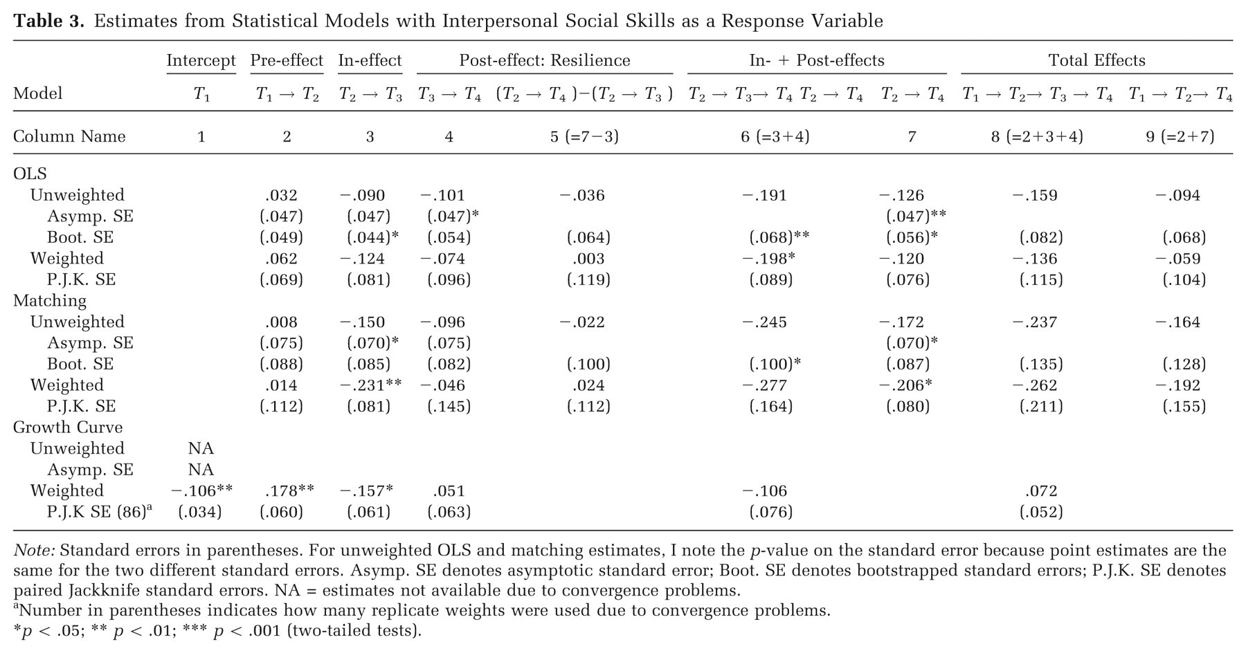
Note: Standard errors in parentheses. For unweighted OLS and matching estimates, I note the p-value on the standard error because point estimates are the same for the two different standard errors. Asymp. SE denotes asymptotic standard error; Boot. SE denotes bootstrapped standard errors; P.J.K. SE denotes paired Jackknife standard errors. NA = estimates not available due to convergence problems.
Number in parentheses indicates how many replicate weights were used due to convergence problems.
p < .05; ** p < .01; *** p < .001 (two-tailed tests).
As children of divorce grappled with their new family contexts, they tended to exhibit declines in interpersonal skills, compared with their counterparts. During the in-divorce stage, children of divorce were more likely to show a relative decline in “forming and maintaining friendships, . . . expressing feelings, ideas, and opinions in positive ways” (Tourangeau et al. 2006:2–23). This finding is quite robust with regard to choice of statistical models (with the exception of the weighted OLS method), providing convincing evidence of the unfavorable effects of parental divorce. The coefficient size of –.231 in the weighted matching method is well over one-third of a standard deviation measured at T 4. Furthermore, statistically significant estimates on the path T 2 → T 4 demonstrate that the adverse effects remain unabated even after children exit the divorce period, although I do not detect stand-alone post-divorce effects. Partly due to the positive figure in the pre-divorce period, however, total divorce effects fall short of statistical significance.
Externalizing behavior problems are also relatively unaffected by parental divorce (see Table 4), regardless of the aggregation and disaggregation of divorce stages (for contrasting results by gender, see Malone et al. 2004). Apart from scattered local instances suggesting a disadvantageous influence of parental divorce, especially in the results of the weighted matching method, there is no consistent and robust evidence to support the traditional hypothesis concerning the negative effects of parental divorce on children’s externalizing behavior. Instead, I see some indications favoring a selection perspective in the results of the growth curve models, as suggested in the estimates of interpersonal skills. In other words, the intercept terms in the trajectories of the growth curves show an elevated initial level of problems among children of divorce in comparison to children in intact families, although a sole estimate of difference in growth over time using the weighted sample reaches statistical significance. The initial gaps persist throughout the study period without widening or shrinking.
Estimates from Statistical Models with Externalizing Problem Behaviors as a Response Variable
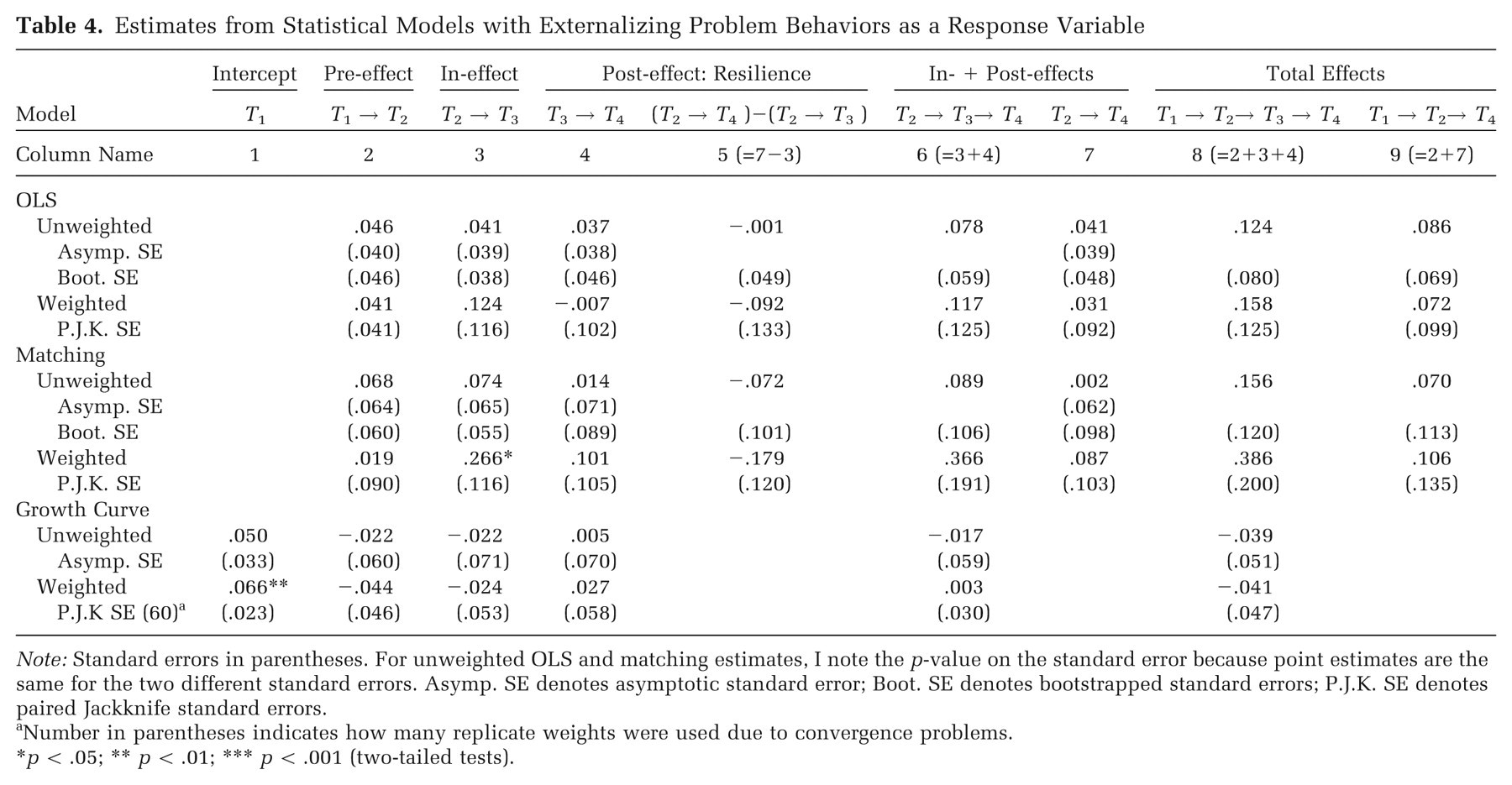
Note: Standard errors in parentheses. For unweighted OLS and matching estimates, I note the p-value on the standard error because point estimates are the same for the two different standard errors. Asymp. SE denotes asymptotic standard error; Boot. SE denotes bootstrapped standard errors; P.J.K. SE denotes paired Jackknife standard errors.
Number in parentheses indicates how many replicate weights were used due to convergence problems.
p < .05; ** p < .01; *** p < .001 (two-tailed tests).
Finally, I turn my attention to differential development in the internalizing behavior domain (see Table 5). Negative consequences of parental divorce are most pronounced during the in-divorce period. Statistically significant point estimates in the neighborhood of one-third to one-half of the population standard deviation (see Table SC-1 in the online supplement) demonstrate conventional consensus concerning the adverse effects of parental divorce on children’s development, at least with regard to internalizing problem behaviors (for contrasting results dependent on timing of divorce, see Lansford et al. 2006). Specifically, compared with their counterparts in intact families, children of divorce were more likely to struggle with “anxiety, loneliness, low self-esteem, and sadness” while their parents were in the divorce stage. Assessment of the subsequent stage indicates that the negative consequences neither disappear nor become exacerbated. A somewhat lower magnitude of estimates for the path T 2 → T 4 and a lack of statistical significance may be suggestive, but only suggestive, of weak resilience at the population level. Total divorce effects are not strong enough to reject the null hypothesis of a zero effect, whether conceptualized via T 1 → T 2 → T 4 or via T 1 → T 2 → T 3 → T 4.
Estimates from Statistical Models with Internalizing Problem Behavior as a Response Variable
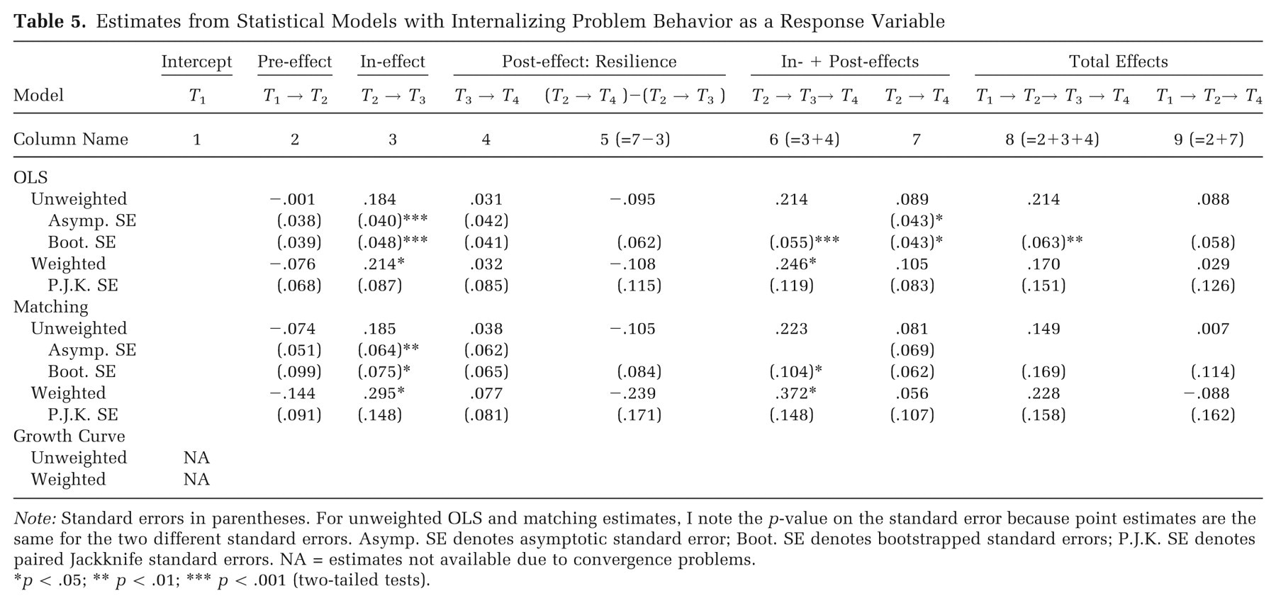
Note: Standard errors in parentheses. For unweighted OLS and matching estimates, I note the p-value on the standard error because point estimates are the same for the two different standard errors. Asymp. SE denotes asymptotic standard error; Boot. SE denotes bootstrapped standard errors; P.J.K. SE denotes paired Jackknife standard errors. NA = estimates not available due to convergence problems.
p < .05; ** p < .01; *** p < .001 (two-tailed tests).
Some additional observations (beyond domain-specific areas) are worth discussing in detail. Coefficients from matching estimators have relatively large absolute values in comparison with those from OLS models, especially for cognitive skill outcomes. From a theoretical point of view, this result is beyond my hypotheses, particularly because the presumably adverse development of intact-family children experiencing high parental conflict, who would be matched with children of divorce experiencing high parental conflict, would ameliorate the negative effects of divorce (Amato et al. 1995). However, I can imagine several reasons for this pattern: (1) measures such as marital happiness and psychological well-being might not capture underlying marital conflict thoroughly; (2) recalling Hanson’s (1999) observation that 75 percent of couples in high conflict remain married, marital conflict may not be the most important predictor of marital dissolution; and (3) the negative effect of “good enough marriages” ending in dissolution could dominate the contrasting force of high-conflict marriages. 10
The empirical results of significant coefficients for math but insignificant estimates for reading are in line with educational literature that suggests the cumulative nature of math and, accordingly, its sensitivity to exogenous impacts (Swanson and Schneider 1999). It is unclear, however, why I find statistically insignificant results for externalizing behavior problems but statistically significant negative results for interpersonal social skills and internalizing behavior problems. From the viewpoint of developmental psychology, stresses and hardships accompanying parental divorce should significantly impair development with regard to all three noncognitive traits (for a theoretical discussion, see Windle [2003]; for empirical evidence, see Kim and colleagues [2003]). I can only suggest that internalizing behavior problems are relatively unstable and sensitive to environmental and extraneous influences, while externalizing behavior problems are stable and insensitive to these factors (Fischer et al. 1984). This interpretation is more convincing considering that I include controls for one-survey-wave lagged outcome variables.
The analyses fail to uncover (1) any consistent pre-divorce effect, (2) resilience parameters at the population level, or (3) definitive total divorce effects. Regarding the pre-divorce effect, several explanations can be offered. First, a two-year in-divorce period might be long enough to include the initiation and development of marital discord, so that some portion of the pre-divorce effect is actually included in the in-divorce effect. Statistically significant in-divorce effects corroborate this point, but descriptive statistics show that marital strain (measured by marital happiness) is already present at T 1 (see Table SC-2 in the online supplement). Second, a one-year window for the pre-divorce period might be too short to capture the pre-divorce effect, not only because children might already have become accustomed to unfavorable daily lives, but also because only a negligible change would take place in such a short period, even though the exogenous shock is substantial. It is also possible that not all divorces are preceded by marital conflict and family dysfunction (Amato 2002; Amato and Booth 1997; Hanson 1999).
On the other hand, parents may decide to dissolve marital relationships only when they see that their children’s development is in line with or more robust than other children and thus have some confidence in their children’s ability to cope with new situations. Conversely, if children show signs of developmental setbacks, parents may maintain marriages to prevent more hazardous consequences. This theoretical position is in accord with the work of Aughinbaugh and colleagues (2005)—both perspectives emphasize the role of rational choice in parents’ decisions—but the perspectives differ in that the former emphasizes parents’ observations of past development rather than a calculation of future outcomes. This temporarily-reversed interpretation of causation seems more congruent with my statistical models, because pre-divorce outcomes measured at T 2 generate the divorce variable rather than the other way around. In addition, an overview of the statistical results across all three stages (i.e., occasional positive pre-divorce effects and some noticeable negative outcomes during the in- and post-divorce periods) appears to be consistent with this interpretation.
Effect parameters for post-divorce impact or resilience, as defined in the theoretical discussion via either T 3 → T 4 or (T 2 → T 4 ) − (T 2 → T 3 ), are not statistically significant, except in a few instances. In contrast to the resilience hypothesis, I find scattered evidence indicating negative post-divorce effects for math test scores and interpersonal social skills. To avoid overstatement or misinterpretation, I caution that the analyses follow children for only two years after divorce, which may be too short a time period to completely recover from the adverse process of parental divorce (Hetherington 2003; Kelly and Emery 2003). Isolating a comparatively more resilient subpopulation and identifying moderating variables that boost or hinder resilience is beyond the scope of this article. Results suggest there is no compelling evidence to support a resilience argument at the population level during the two years following divorce.
Imprecise estimates of the pre- and post-divorce effects appear to be responsible for the statistically insignificant total divorce effects. To avoid the impression that statistically insignificant total divorce effects may suggest a rejection of the negative divorce effects hypothesis, I stress that the pre-divorce parameters assessed here lack causal interpretation. Therefore, the term “total effects” as defined here should not be interpreted as the sum of causal effects across all dissolution stages. In this sense, discovery of combined effects of the in- and post-divorce stages in several important developmental domains should be considered “total divorce effects” in its literal meaning, because these parameters are considered causal. Furthermore, absence of a post-divorce effect, combined with the presence of a negative in-divorce effect, suggests a continuing, if not increasing, developmental gap between children of divorce and children with continuously married biological parents. If pre-divorce effects actually represent the selective decisions of parents with robustly developing children to dissolve a marriage, my findings on in- and post-divorce effects would be more consistent with the traditional findings of negative divorce effects, although the results would be confined to certain developmental domains.
Discussion and Conclusions
This article examined the effects of parental divorce on several childhood developmental domains within three analytically distinct divorce stages: pre-, in-, and post-divorce. Using several statistical methods, I found that effects of parental divorce are stage- and domain-specific. To summarize, I found (1) setbacks among children of divorce in math test scores during and after the experience of parental divorce (i.e., significant combined effects of the in- and post-divorce effect), (2) a negative in-divorce effect on interpersonal skills and negative combined effects during the in- and post-divorce periods, and (3) a pronounced in-divorce effect on the internalizing behavior dimension. However, (4) I found no negative consequences of parental divorce for reading test scores, nor did I find an increase in externalizing behavior problems in any stage. Additionally, (5) I did not find statistically significant estimates of a pre-divorce effect, a resilience parameter at the population level, or a total divorce effect as defined herein.
A discussion of several limitations of this article is necessary to properly evaluate its contributions and to delineate future tasks for a more sophisticated and meaningful research program. I am primarily concerned with possible confounding by unobserved covariates, a thorny issue shared by all observational data analyses (Rosenbaum 2002). All of the statistical techniques employed in this article are subject to unobserved confounding bias to varying degrees; even the weighting method used to account for longitudinal attrition is based on the assumption of fully observed covariates.
Probable measurement error in the noncognitive trait scales is another limitation, even though literature on children’s mental health tends to agree on the usefulness of teacher reports (e.g., see Verhulst, Koot, and Van der Ende 1994). The measures of noncognitive traits may be disputable not only because they were computed as an average of several individual items, but also because they were assessed by different teachers across longitudinal survey waves. Data collectors also cautioned against building longitudinal models with noncognitive traits as response variables (Tourangeau et al. 2006). Estimates in this article should therefore be considered one plausible test at the current stage rather than definitive support for or against specified hypotheses.
Because the analyses followed children for only two years after parental divorce, neither latent negative effects nor resilience effects could be fully observed. As Cherlin (2008) notes, effects of parental divorce may be latent because devastating results may be entirely realized only after children of divorce grow up or encounter significant social events, such as their own marital decisions (see also Wallerstein and Lewis 2004). While there is some agreement that a negative in-divorce effect reflects a meaningful impact, some scholars maintain the opposing perspective that most children recover from devastating experiences as time passes (Hetherington 2003; Kelly and Emery 2003). The current analyses do not support either view, but ECLS-K is an ongoing survey, allowing further opportunities to rigorously validate or invalidate these theoretical propositions.
Finally, the results presented here are confined to children who experienced the divorce of two biological parents during the period between spring of 1st grade and spring of 3rd grade, and who were 7 to 9 years and 9 to 11 years in respective survey points. This limitation means the results may not apply to children who experience parental divorce in early childhood or adolescence. One study suggests stronger effects in younger children (age 0 to 5 years) as opposed to older children (6 to 10 or 11 to 16 years), with some variations depending on outcome variables (Allison and Furstenberg 1989). In a related vein, Amato (1993) notes that age at parental divorce is likely related to different types of risks in developmental outcomes. For instance, children in early childhood are supposedly less sensitive to environmental changes, particularly involving emotional reconfiguration, compared with adolescents (Papalia, Olds, and Feldman 2004; for a meta-analysis, see Amato [2001]). These observations preclude unwarranted generalization of the current results and call for an extension of the analytic framework to improve scholarly understanding of divorce and the development of affected children.
Footnotes
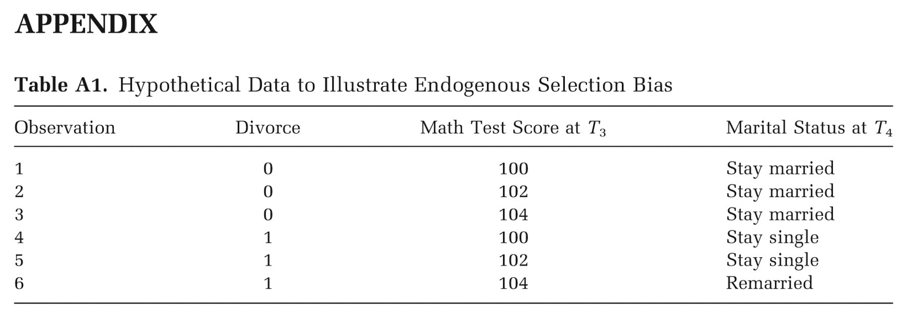
Appendix
Hypothetical Data to Illustrate Endogenous Selection Bias
| Observation | Divorce | Math Test Score at T 3 | Marital Status at T 4 |
|---|---|---|---|
| 1 | 0 | 100 | Stay married |
| 2 | 0 | 102 | Stay married |
| 3 | 0 | 104 | Stay married |
| 4 | 1 | 100 | Stay single |
| 5 | 1 | 102 | Stay single |
| 6 | 1 | 104 | Remarried |
Acknowledgements
A draft of this article was presented at the 2010 annual meeting of the Population Association of America at Dallas, Texas. I am grateful to five anonymous reviewers whose constructive comments substantially improved this article. Thanks to Chaeyoon Lim, Felix Elwert, John A. Logan, and Robert M. Hauser who provided helpful comments throughout the development of this article.
1.
As is the convention in the literature, I do not distinguish separation from divorce (Amato 2001; ![]() ). I use the more generic term “divorce” throughout this article unless otherwise noted.
). I use the more generic term “divorce” throughout this article unless otherwise noted.
2.
For examples using an OLS framework, see references in Amato and Keith (1991) and Amato (2001); for a matching method study, see Frisco, Muller, and Frank (2007); for a fixed-effects model, see Aughinbaugh, Pierret, and Rothstein (2005); for a study using behavioral genetics methods, see D’Onofrio and colleagues (2006); and for other invaluable study designs, see ![]() .
.
3.
4.
At the time analysis for this article was completed, 8th grade data were not available.
5.
To illustrate endogenous selection bias, consider the hypothetical six observations in Table A1 of the Appendix. If I used all observations, I would find no effect of divorce on math test scores. If I selected respondents who remained single at T 4, the divorce effect would be calculated as –1.
6.
Parent-assessed social rating scales are not available for T 3 and T 4 survey waves.
7.
The data collector releases only the mean for entire classes of submeasures.
8.
Conditioning on school moves may lead to an underestimation of divorce effects, as the theoretical discussion indicated. However, a recent article by ![]() demonstrates that geographic relocation enhances the risk of marital dissolution. Failure to find a better proxy for geographic relocation leads me to use school moves between adjacent interview waves. I also conducted OLS analyses without the school move variable and found quantitatively negligible differences and qualitatively identical conclusions (estimates available from the author on request).
demonstrates that geographic relocation enhances the risk of marital dissolution. Failure to find a better proxy for geographic relocation leads me to use school moves between adjacent interview waves. I also conducted OLS analyses without the school move variable and found quantitatively negligible differences and qualitatively identical conclusions (estimates available from the author on request).
9.
Among the 142 children of divorce, the custodial mother or father of 103 children remained single at T 4, while 21 children experienced parental remarriage or cohabitation, and the remaining 18 children had unidentifiable information on parents’ marital status. When weighted, these groups are 67.0, 24.4, and 8.6 percent of the sample, respectively.
10.
To further explore these ideas, I present matching estimates by marital happiness level reported by divorced parents at T 1 in Table SD-1 of the online supplement. Although not entirely consistent across developmental domains and time dimensions, divorce effects appear most pronounced in children of divorce whose parents’ marriages were “not too happy (0).” These results support the first and second speculations rather than the last one.
References
Supplementary Material
Please find the following supplemental material available below.
For Open Access articles published under a Creative Commons License, all supplemental material carries the same license as the article it is associated with.
For non-Open Access articles published, all supplemental material carries a non-exclusive license, and permission requests for re-use of supplemental material or any part of supplemental material shall be sent directly to the copyright owner as specified in the copyright notice associated with the article.