
Abstract
This article seeks to experimentally evaluate the thesis that marriage is deinstitutionalized in the United States. To do so, we map the character of the norm about whether different-sex couples ought to marry, and we identify the extent to which the norm is strong or weak along four dimensions: polarity, whether the norm is prescriptive, proscriptive, bipolar (both prescriptive and proscriptive), or nonexistent; conditionality, whether the norm holds under all circumstances; intensity, the degree to which individuals subscribe to the norm; and consensus, the extent to which individuals share the norm. Results of a factorial survey experiment administered to a disproportionate stratified random sample of U.S. adults (N = 1,823) indicate that the norm to marry is weak: it is largely bipolar, conditional, and of low-to-moderate intensity, with disagreement over the norm as well as the circumstances demarcating the norm. While the norm to marry is different for men and women and for Black and White respondents, the amount of disagreement (or lack of consensus) within groups is comparable between groups. We find no significant differences across socioeconomic status (education, income, and occupational class). Overall, our findings support key claims of the deinstitutionalization of marriage thesis.
Where does the institution of marriage stand in the mind of the American public? There is growing consensus among family scholars that the institution of marriage is experiencing profound changes (Cherlin 2004, 2020; Coontz 2005; Knapp and Wurm 2019; Lundberg and Pollak 2007; Lundberg, Pollak, and Stearns 2016; Powell et al. 2010; Rosenfeld 2007; Thornton, Axinn, and Xie 2007). In a programmatic statement, Cherlin (2004:848) refers to the sum of these changes as the deinstitutionalization of marriage, or “the weakening of the social norms that define people’s behavior in a social institution such as marriage.” Cherlin’s (2004, 2020) deinstitutionalization of marriage thesis maintains that the institution of marriage is undergoing uneven declines across social groups. While marriage still plays a central role for White Americans and the college-educated, Cherlin (2020) contends that alternatives to marriage have become more acceptable and are more prevalent among Black Americans and the non-college-educated, suggesting that the norm about whether to marry has weakened. 1
At the heart of the deinstitutionalization of marriage thesis are empirical questions about the “strength” of social norms governing marriage. Common definitions of a social norm conceptualize it as a rule, with some degree of consensus, that prescribes or proscribes a particular action (Coleman 1990; Hechter and Opp 2001; Horne 2009). Given this definition, what constitutes a strong or weak norm? For Cherlin (2020:64), a norm is strong when it is “widely agreed upon,” and a norm is weak when there is widespread disagreement. Yet the literature on social norms suggests a norm can be strong or weak along four dimensions (Horne, Dodoo, and Dodoo 2018; Jackson 1966; Jasso and Opp 1997; Rauhut and Winter 2010; Rossi and Berk 1985): polarity, whether a norm for a given individual is prescriptive (permit and endorse behavior), proscriptive (prohibit and oppose behavior), bipolar (both prescriptive and proscriptive), or nonexistent (an individual does not subscribe to the norm); conditionality, whether a norm for a given individual holds under all or some circumstances; intensity, the degree to which an individual subscribes to a norm; and consensus, the extent to which members of a population share a norm. Investigating each of these dimensions—particularly whether there is consensus across racial and socioeconomic lines—is necessary to assess the deinstitutionalization of marriages thesis.
Prior research examining norms about marriage has yet to measure all four dimensions in a single study, which makes it difficult to evaluate the strength of social norms surrounding the institution of marriage in general and the deinstitutionalization of marriage thesis in particular. In the current study, we address this gap by designing a factorial survey experiment (FSE) of different-sex marriage (Auspurg and Hinz 2015): a method that leading scholars of social norms argue is more systematic and better suited to measuring social norms than are conventional survey items or ethnographic methods (Horne, Dodoo, and Dodoo 2013; Horne et al. 2018; Jasso 2006; Jasso and Opp 1997). To test whether the norm to marry differs across social groups, we administer our FSE to a random sample of U.S. adults disproportionality stratified by race (Black, White), gender (male, female), and education (high school diploma, some college, bachelor’s degree or higher).
With this design, we provide a comprehensive evaluation of Black and White Americans’ approval of different-sex marriage, how conditional that approval is on the characteristics of those getting married, and how much consensus there is within and between demographic groups. Most importantly, the proposed FSE eliminates problems of internal validity inherent in observational studies via random assignment. Marriage conditions and preferences that are correlated in real life, such as education and earnings, are orthogonal by design in our experiment. We can thus untangle effects of circumstances that commonly co-occur, permitting us to test and directly compare the independent effects of conditions that demarcate the norm to marry. Moreover, because we oversample specific demographic groups (e.g., Black Americans, the college-educated), we can better test whether theorized differences exist between subpopulations, particularly Black Americans and White Americans and the non-college-educated and college-educated (Cherlin 2004, 2020). We can also draw population-based inferences for these randomly sampled subpopulations.
In short, this article makes two contributions. First, it contributes to family scholarship by directly measuring the four dimensions of the norm to marry; by investigating the extent to which the norm to marry varies across demographic groups; and by applying these methods and forms of investigation to a disproportionate stratified random sample of U.S. adults. Second, it extends the literature on social norms to a new area of study, illustrating how the conceptualization and measurement of social norms can provide novel insights in other fields like marriage and the family.
Our findings show that the majority of Black and White respondents in the United States embrace a different-sex marriage norm. Yet the norm to marry is weak: it is largely bipolar, conditional, and of low-to-moderate intensity, with disagreement over the norm as well as the circumstances demarcating the norm. Our results buttress most claims of Cherlin’s (2004, 2020) deinstitutionalization of marriage thesis: the norm to marry is weak and divided along racial and gender lines, although not by socioeconomic status (SES).
Social Norms and the Norm to Marry: Theoretical and Empirical Background
Four Aspects of a Social Norm
A social norm is a rule about a particular behavior, with some degree of consensus, that is socially enforced (Coleman 1990; Hechter and Opp 2001; Horne 2009). Rules—the backbone of social norms—are statements “claiming that something ought or ought not to be the case” (Opp 2013:384). This implies that rules prescribe (permit) or proscribe (prohibit) particular actions (behaviors to which a social norm applies), and that individuals who subscribe to a norm tend to punish those who violate the rules and reward those who follow the rules (Coleman 1990; Hechter and Opp 2001; Horne 2009). As Bicchieri (2006:42) writes: “Social norms prescribe or proscribe behavior; they entail obligations and are supported by normative expectations. Not only do we expect others to conform to a social norm; we are also aware that we are expected to conform, and both these expectations are necessary reasons to comply with the norm.”
These definitions highlight four key aspects of a social norm (Grigoryeva and Robbins 2021; Horne et al. 2018; Jackson 1966; Jasso and Opp 1997; Rauhut and Winter 2010; Rossi and Berk 1985). First, norms might vary in their polarity: they can be prescriptive, proscriptive, bipolar, or nonexistent. Second, norms might vary in their conditionality: they can hold under all (unconditional) or some (conditional) circumstances. Third, norms might vary in their intensity: individuals can differ in the degree to which they subscribe to a norm (e.g., low, moderate, or high). Fourth, norms might vary in their level of consensus: they can be shared by all or only a few members of society.
Polarity
The first step in establishing how strong or weak a social norm is in a population is to examine the norm’s character for each individual. Mapping the character of a norm begins by identifying its polarity. Polarity means that for any given individual, a person can uniformly oppose a focal action or behavior regardless of the circumstances (proscriptive), uniformly endorse a behavior regardless of the circumstances (prescriptive), oppose and endorse a behavior depending on the circumstances (bipolar), or neither oppose nor endorse a behavior as there may not be a norm or rule guiding the focal action (nonexistent).
Conditionality
One should also evaluate whether the norm under study is unconditional—“under no circumstance should an individual perform X” or “under all circumstances should an individual do X”—and, if not, in which conditions does the social norm apply. Most norms are replete with conditions. Even a seemingly universal norm such as “thou shalt not kill” can have limits placed on the conditions in which it does or does not hold. Killing in some cultures is appropriate when in self-defense or when the victim is an outgroup member (e.g., White Americans lynching Black Americans in the U.S. South during Jim Crow).
Conditionality is thus the degree to which a social norm—for any given individual—holds under all circumstances, where circumstances refer to characteristics of the situation or the situations’ interactants. Whereas polarity implies direction, conditionality identifies the degree to which individuals vary in their evaluation of a norm in light of shifting circumstances. For instance, individual A might uniformly prescribe marriage, but nonetheless vary the magnitude of her prescriptions depending on the circumstances. Individual B, in contrast, might uniformly prescribe marriage to the same degree regardless of the circumstances. In these examples, individual A subscribes to a conditional norm, whereas individual B subscribes to an unconditional norm. For any individual, an unconditional norm may be prescriptive or proscriptive, but never bipolar; a conditional norm, in contrast, may be prescriptive, proscriptive, or bipolar. Thus, a bipolar norm is always a conditional norm by definition.
Intensity
Whereas polarity identifies the direction of a social norm, intensity is the degree to which an individual subscribes to a norm. For instance, individuals A and B might both uniformly prescribe marriage, but the degree of this prescription could be “not very strong at all” for individual A and “very strong” for individual B. Individual A and individual B both feel obligated to conform to the norm to marry, but the magnitude of each individual’s personal obligations and expectations varies.
Consensus
Polarity, conditionality, and intensity are first established at the individual level, and then proportions and central tendencies can be used to map their distributions in the population. Consensus, by contrast, refers to the degree to which individuals in the population share a norm: the degree of unanimity in the knowledge of a rule, common preferences to conform to a rule, and shared expectations of others’ conformity to a rule. In other words, consensus can “be described as the homogeneity of acceptance concerning the validity of one particular norm within a population” (Rauhut and Winter 2010:1183, emphasis added). Consensus is demonstrated by identifying the extent to which a norm is shared within and between subpopulations, and it ultimately rests on the amount of between-individual variation in a norm (Jasso 2006).
Consensus is crucial for understanding the shared character of a norm in a population. Some norms vary between subpopulations but not within, and other norms vary to a great extent within and between subpopulations. Gaining knowledge of how a norm is shared in a population specifies how strong or weak a norm might be. For instance, if half the individuals in a population uniformly prescribe marriage and the other half uniformly proscribe marriage, this would suggest disagreement (or a lack of consensus) in the norm to marry. Given disagreement in the population, the next step is to identify which traits or characteristics are common among subpopulations (e.g., upper-middle-class individuals might be more likely to prescribe marriage than would individuals in poverty).
Theoretically, a strong norm is one with consensus about a rule that approves (or disapproves) of a particular behavior, where the strength of approval (or disapproval) is intense and the circumstances under which the rule applies are unconditional. One ideal-typical strong norm is a norm against incest: individuals widely believe, to a great degree, that incest is strictly prohibited regardless of the conditions. A weak norm, by contrast, is one with widespread disagreement in which (1) some people approve of a particular behavior, others disapprove, and still others might believe the focal action is not guided by rules, (2) the strength of approval or disapproval is mild, and/or (3) the circumstances under which the rule applies are varied. The norm about whether and what to give on Valentine’s Day is a contemporary example of a weak norm: some people feel obligated to give a gift, other people refuse to participate in the tradition out of principle, and most people do not care either way.
Despite their importance, these four dimensions are rarely used to shed light on topics of general interest to sociologists (for exceptions, see Horne et al. 2018; Jasso and Opp 1997; Rauhut and Winter 2010). The primary reason for this is methodological. Although sociologists have toolkits for inferring the representativeness of various attitudes, beliefs, and intentions—such as general social surveys—widespread measurement of the four dimensions of social norms is lacking. To properly measure polarity, conditionality, intensity, and consensus, respondents must assess a systematic set of counterfactual conditions, which is time-consuming and costly for general population surveys. However, because norms undergird most social institutions, questions of broad sociological interest—such as the deinstitutionalization of marriage thesis (Cherlin 2004, 2020)—would benefit from theoretical insights and methodological tools developed by scholars of social norms. This article offers a template for incorporating the four dimensions of social norms into sociological research, and extends the empirical scope of the multidimensional approach to measuring norms.
The Norm to Marry in the United States
In the United States, social norms have long played a part in individual decisions to marry (Edin and Kefalas 2005; Powell et al. 2010; Rosenfeld 2007). Measuring the norm about whether different-sex couples ought to marry is thus important for the resolution of debates over the polarity, intensity, conditionality, and consensus of the norm. We briefly review these major debates and findings. 2
Polarity and intensity
Although we cannot document change over time, we contextualize our work by noting that throughout much of the twentieth century prior to the 1960s, only about 5 percent of people in the United States ever cohabited, and couples would typically marry after roughly six months of dating (Coontz 2005; Cott 2002). This suggests that social norms at the time were prescriptive of marriage following a narrow dating period. Individuals today, however, are less likely to think that couples should marry, and people have a greater tolerance for behaviors that were once forbidden socially (Powell et al. 2010). Americans’ attitudes toward marriage have also grown more negative, and they view marriage as more restrictive (Gubernskaya 2010; Thornton and Young-DeMarco 2001; Treas, Lui, and Gubernskaya 2014). Despite shifts in attitudes and behavior, the literature suggests that norms still govern marriage in the contemporary United States (Cherlin 2020; Knapp and Wurm 2019; Lauer and Yodanis 2010), although norms may be less prescriptive, less intense, and more conditional than they were in the past. In other words, the normative pressure to marry may still exist, but be less absolute, applying to fewer situations and couples than before.
This article offers a thorough assessment of whether individuals in the contemporary United States—particularly Black Americans and White Americans, and the non-college-educated and college-educated—think that different-sex couples should or should not marry. Unlike previous work, we can answer the following questions: Is the contemporary norm to marry in the United States prescriptive, proscriptive, bipolar, nonexistent, or some combination of the four? Among those who subscribe to a norm (be it prescriptive, proscriptive, or bipolar), what is the magnitude or intensity of their devotion? Finally, how important are conditions for understanding these norms?
Conditionality: economic bar to marriage
One important circumstance serving as a boundary of different-sex marriage, revealed by both quantitative and qualitative research, is that individuals need to meet a set of economic goals in order to marry (Edin 2000; Edin and Kefalas 2005; Gassman-Pines et al. 2017; Gibson-Davis, Gassman-Pines, and Lehrman 2018; Ishizuka 2018; Rackin and Gibson-Davis 2017; Schneider 2011; Watson and McLanahan 2011). Some research finds that men’s and women’s earnings and financial contributions are both important for entry to marriage (Gibson-Davis et al. 2018; Ishizuka 2018; Kuo and Raley 2016), but earlier research suggests that men’s financial position and economic prospects are more important than women’s (Gibson-Davis 2009; Smock et al. 2005). Beyond earnings and employment prospects, assets are also tied to marriage (Schneider 2011); that is, couples believe they should have the necessary capital or wealth to afford various “capstone” events, such as a wedding or homeownership (Edin and Kefalas 2005; Gibson-Davis 2018; Smock, Manning, and Porter 2005). An economic bar to marriage is one potential explanation for why low-income individuals are less likely to marry than other socioeconomic groups (Watson and McLanahan 2011). Our research can help clarify the importance of economic features relative to other relationship features, and whether men’s and women’s financial achievements are similarly important for prescribing different-sex marriage.
Conditionality: pregnancy status
A strong norm forbidding nonmarital childbearing existed in the United States until the last third of the twentieth century; this norm is still observed, albeit in a weakened state and with variation across subpopulations (Barber, Yarger, and Gatny 2015; Cherlin et al. 2008; Daughterty and Copen 2016). Although research on low-income parents suggests this norm has declined, ethnographic research shows that low-income individuals without children view marriage and childbearing as strongly coupled (Rackin and Gibson-Davis 2017). Likewise, the prevalence of “shotgun marriages” has remained relatively stable over time (Gibson-Davis, Ananat, and Gassman-Pines 2016), and the majority of U.S. adults agree that people who want children should marry (Thornton and Young-Demarco 2001). It is thus an open question about how strong prescriptions to marry are when couples face a pregnancy. Our research can help answer this question.
Conditionality: relationship quality
What constitutes relationship quality, and the level required for entry into marriage, has likely shifted. Marriage in the United States has moved from companionate marriages (in which quality means emotional satisfaction from playing marital roles well) to individualized marriages (in which quality means self-fulfillment, openness, and communication) (Cherlin 2004, 2010; Lesthaeghe 2014). These shifts suggest that whether people should marry depends on the quality of their relationship. Brown (2004) finds that relationship quality does not increase the likelihood of marriage among cohabiting couples, but other research finds that distrust and conflict reduce the likelihood of marriage (Waller and McLanahan 2005). One goal of our study is to identify the extent to which relationship quality matters as a circumstance demarcating who should or should not marry.
Consensus: race, gender, and socioeconomic status
A central goal for family scholars has been to understand the growing divergence in the institution of marriage across subpopulations (Pagnini and Morgan 1996; Wilson 1987, 1996, 2009). White Americans and the college-educated are more likely to marry and hold favorable attitudes toward marriage than are Black Americans and the non-college-educated, respectively (Gubernskaya 2010; Kuo and Raley 2016; Lundberg and Pollak 2007; Raley, Sweeney, and Wondra 2015; Sassler and Schoen 1999; South 1993; Torr 2011). 3 Women are also more likely than men to prefer marriage, and are more certain about their desire to get married (Thornton and Young-DeMarco 2001). Other research, however, shows that women report stronger negative attitudes toward marriage than do men (Autor and Wasserman 2013; Gubernskaya 2010; Sassler and Schoen 1999).
Finally, a sizable body of research suggests that Black Americans and White Americans, as well as the non-college-educated and college-educated, disagree over the circumstances demarcating marriage, namely the economic bar, pregnancy status, and relationship quality (Cherlin et al. 2008; Edin 2000; Edin and Kefalas 2005; Gibson-Davis, Edin, and McLanahan 2005; Rackin and Gibson-Davis 2017; Smock et al. 2005; Waller 2002; Wilcox and Wolfinger 2016). In short, divergences along racial, gender, and socioeconomic lines have created disagreement over the institution of marriage in the United States. Our research design allows us to assess whether there is, in fact, a lack of consensus in the norm to marry, as well as the circumstances governing the norm.
Research Questions
The goal of this study is to evaluate the strength of the norm about whether different-sex couples ought to marry in the United States. We do so by mapping the character of the norm and by establishing whether divergent subsystems of the norm exist across race (Black, White), gender (male, female), and SES (education, income, occupational class).
We follow Jasso and Opp’s (1997) method of mapping the character of a social norm; that is, we investigate the polarity, conditionality, intensity, and consensus of the norm to marry. Given the results, we then investigate the circumstances in which the norm to marry holds and whether these circumstances vary by subgroups in the U.S. population. This includes measuring the existence of the following conditions: different-sex couples ought (or ought not) to marry (1) unless they have achieved a certain economic status, (2) when they are expecting a child, and (3) when the quality of their relationship is good. Given the goals specified earlier, we use the following questions to orient our study:
Question 1. What is the character (polarity, conditionality, intensity, consensus) of the norm to marry among Black and White Americans in the United States, and what does it imply for the deinstitutionalization of marriage thesis?
Question 2. What are the circumstances demarcating, or serving as boundaries of, the norm to marry among Black and White Americans in the United States?
Question 3. Are individual tendencies to proscribe or prescribe marriage universal or specific to subpopulations based on race (Black, White), gender (male, female), or SES (education, income, occupational class)?
Question 4. Are circumstances demarcating the norm to marry universal or specific to subpopulations based on race (Black, White), gender (male, female), or SES (education, income, occupational class)?
Data and Methods
To measure the character of the norm to marry, we use an FSE design (Auspurg and Hinz 2015; Jasso 2006). The typical FSE presents respondents with hypothetical scenarios (vignettes) that reflect real-life situations and stimuli. Within each scenario or vignette, experimenters manipulate attributes of the situation (dimensions) by randomly assigning attribute values (levels) to elicit judgments, decisions, or intentions with one or more dependent variables (evaluation task). In this study, we presented a disproportionately stratified random sample of U.S. adults with 10 vignettes describing a fictive couple, Mike and Jessica. 4 We used a number of norm-relevant dimensions, such as Mike’s and Jessica’s individual earnings, to characterize their circumstances. Each dimension consisted of two or more manipulated levels (e.g., $20,000 versus $50,000 in earnings) that we randomly assigned to respondents. We then asked respondents to evaluate and judge whether the protagonists in each vignette ought to or ought not to marry.
The Respondent Sample
The sample consisted of respondents drawn from a nationally representative web panel collected by GfK (formerly Knowledge Networks). Participants for the study came from a random subset of the GfK web panel, which was recruited using a combination of list-assisted random-digit dial and address-based sampling methods. The study was fielded in January 2017 and targeted English-speaking, non-institutionalized adults age 18 and older residing in the United States. GfK contacted 3,181 web panel participants; 1,823 participants completed the study, yielding a 57 percent completion rate.
One goal of our study was to investigate whether the norm to marry is universal or specific to subpopulations based on race, gender, or SES. We thus designed our sample to create 12 different demographic cells cross-classified by race, gender, and SES, with roughly 150 observations per cell. We restricted the sample to non-Hispanic White and non-Hispanic Black individuals (henceforth White and Black, respectively), with an oversample of Black respondents. We measured and restricted gender to males and females. Highest educational attainment was categorized as high school diploma, some college, and bachelor’s degree or higher. The “high school diploma” category consists of respondents who received a high school diploma, GED, or high school equivalence certification. The “some college” category consists of respondents who received an associate’s degree or completed some college courses but did not receive a degree. The “bachelor’s degree or higher” category consists of individuals who had graduated with a bachelor’s, master’s, professional, or doctorate degree. Our sample excludes respondents without a high school diploma because GfK was unable to guarantee a sufficient number of Black males or Black females with only some high school. 5 Given our stratified sample design and budget constraints, we chose to maximize sample size—and consequently statistical power—for cells that GfK was able to guarantee a sufficient number of observations.
In all, our survey includes 911 male, 912 female, 913 Black, 910 White, 609 high school diploma, 608 some college, and 606 bachelor’s degree or higher respondents. The result is 12 different demographic cells (e.g., Black male with a high school diploma) with roughly 150 observations per cell. Other key demographic characteristics—such as age, census region, and metropolitan area—are representative of the U.S. population.
Demographic Characteristics
Socioeconomic status
We utilized two additional indicators to measure SES. First, we used respondents’ household income. To measure household income, we took the midpoints of closed income categories provided by GfK. We then adjusted for household size (divided midpoint values by total household size) and natural logged the adjusted values. This produced a logged per capita household income adjusted for household size.
Second, we used a modified version of the EGP class schema (Erikson and Goldthorpe 1992) to create an occupational-based measure of social class, hereafter “occupational class”: class one (higher- and lower-grade professionals, administrators, managers, and officials), class two (routine nonmanual and service employees, higher- and lower-grade), class three (high-grade technicians and repairers, public safety workers, performers, and supervisors of manual workers), class four (skilled manual workers, lower-grade technicians, installers, and repairers), class five (semi-skilled and unskilled manual workers, not in agriculture), class six (agricultural), class seven (military), other occupation (occupation unknown), not working (layoff, looking for work, and other not working), retired, and disabled.
Control variables
To account for possible confounding at the individual-level, we controlled for various attitudes and demographic characteristics: age, marital status, cohabitation status, housing type, ownership of living quarters, MSA status, region, religious affiliation, religiosity, religious attendance, a short-form GSS vocabulary test, and marriage judgments. We omitted estimates of the control variables from all tables to conserve space, because our focus is on testing whether the norm to marry varies by race, gender, or SES. Given the centrality of some control variables in debates about marriage (e.g., religion), we include estimates of all control variables in the online supplement. Summary statistics and descriptions of all individual-level variables used in the present study are in Appendix Table A1.
The Vignette Samples
Vignette dimensions and levels
In an FSE, “the choice of vignette characteristics is based on the conjecture that the characteristics may be relevant in the eyes of some respondents” and that the vignette characteristics capture “potentially normatively relevant information” (Jasso and Opp 1997:951). Thus, the first step in constructing our FSE was to select circumstances relevant to setting the norm’s boundaries. Our decision was based on three separate sources of information. First, we followed recent prescriptions offered by FSE methodologists who suggest the number of dimensions to include in an FSE should be greater than four but less than ten (Auspurg and Hinz 2015). This nine-to-five range undermines order effects (i.e., bias that results from the order in which a dimension is presented in a vignette), reduces respondent boredom and fatigue effects, and facilitates unbiased evaluation of vignettes for respondents of higher age (over 60 years old), lower educational background, and little familiarity with the topic under evaluation. Second, our decision was also informed by a pretest administered to undergraduate students at a large public university (N = 75), a focus group of undergraduate honors students (N = 15), and a pilot study of Amazon.com Mechanical Turk workers (N = 530). 6 Third, and most importantly, we were guided by the previously reviewed literature on the norm to marry in the United States.
Given the literature and our extensive pretesting, we manipulated seven vignette dimensions (see Table 1), consisting of pecuniary and non-pecuniary characteristics of Mike, Jessica, and their relationship. To avoid number-of-level effects (see Auspurg and Hinz 2015:20), we restricted the number of levels manipulated per dimension to no more than three. Following convention (Wallander 2009), our manipulated levels include high and low values or the presence and absence of vignette characteristics.
Norm to Marry Vignette Dimensions and Levels
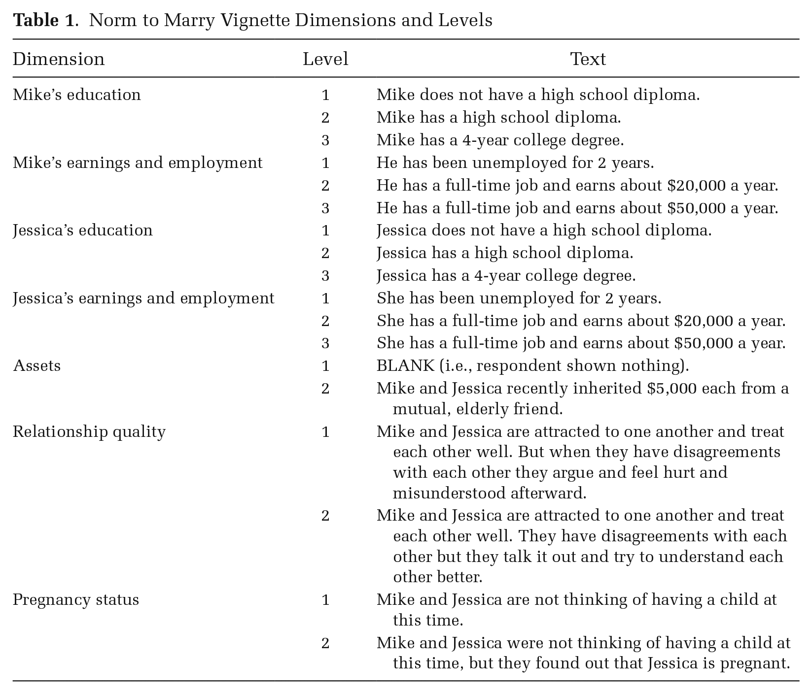
Research consistently finds that an economic bar must be met before marriage is judged desirable (Edin 2000; Edin and Kefalas 2005; Gassman-Pines et al. 2017; Gibson-Davis et al. 2018; Ishizuka 2018; Rackin and Gibson-Davis 2017; Watson and McLanahan 2011). The most basic characteristics behind the economic bar to marriage are the earnings, employment, and education of male and female partners. For earnings and employment, we distinguish between unemployment (“she/he has been unemployed for 2 years”) and two earnings levels (“she/he has a full-time job and earns about $20,000/$50,000 a year”) for both Mike and Jessica. 7 The control level (i.e., unemployment) describes situations of relatively low economic standing, and the middle (i.e., “earns about $20,000”) and upper levels (i.e., “earns about $50,000”) represent roughly the first quartile and median income, respectively, for male householders (no wife present) in the United States (DeNavas-Walt, Proctor, and Smith 2012). Building from the same literature, the education of Mike and Jessica includes three levels roughly corresponding to SES in the United States: “Mike/Jessica . . . does not have a high school diploma/. . . has a high school diploma/. . . has a 4-year college degree.” Although higher levels of education can be achieved, we manipulated these three levels as they constitute the bulk of education levels observed in the U.S. population. Taken together, earnings and employment consist of two dimensions (one for Mike and one for Jessica), as does education (one for Mike and one for Jessica).
We used the final pecuniary characteristic, assets, to capture the money needed to be in place for individuals to marry (Edin and Kefalas 2005; Schneider 2011; Smock et al. 2005). For our assets dimension, one level was mentioned in the vignettes (“Mike and Jessica recently inherited $5,000 each from a mutual, elderly friend”), and the other level was not (i.e., a blank level). We settled on this operationalization of assets to reduce measurement confounding. Assets that are accrued exogenously (i.e., inheritance from a friend) are not correlated with other features of Mike or Jessica, such as motivations to save money or the accrual of debt.
Many non-pecuniary characteristics inform decisions to marry, including control over household decisions, fear of domestic violence, and drug use (Edin 2000; Edin and Kefalas 2005; Smock et al. 2005). For the current study, we focus on two classic characteristics: relationship quality and pregnancy status. Relationship quality is often viewed as a multidimensional construct that consists of objective and subjective characteristics, such as levels of companionship, communication, affection, trust, and conflict, as well as satisfaction and happiness with the relationship (Wilcox and Nock 2006). Investigating several aspects of relationship quality would require too many vignette dimensions. Instead, we focus on communication and conflict. Therefore, two levels that emphasize (a lack of) communication and conflict resolution operationalize relationship quality (see Table 1).
To see whether unmarried couples are expected to marry given a pregnancy, we distinguish between not pregnant (“Mike and Jessica are not thinking of having a child at this time”) and pregnant (“Mike and Jessica were not thinking of having a child at this time, but they just found out that Jessica is pregnant”). The goal of our operationalization was to provide respondents with Mike and Jessica’s preferences for children (not now, but possibly later) as well as their pregnancy status (not pregnant versus pregnant).
Population of vignettes
With the vignette dimensions and levels outlined in Table 1, we constructed the factorial object universe or vignette population (i.e., all possible combinations of dimensions and levels). The number of possible vignettes (V) is 23 × 34 = 648. Because all possible vignettes were plausible and logical, the resulting factorial object universe did not result in impossible combinations of dimensions and levels. As a result, we retained the full population of 648 vignettes.
Drawing vignette samples
The final two design-based choices involved the number of vignettes to present to respondents and the sampling procedure used to assign vignette dimensions and levels to respondents.
With respect to the number of vignettes, the methodological literature suggests that respondents should evaluate no more than 10 vignettes to avoid cognitive overload, fatigue, and learning effects (Auspurg and Hinz 2015). Evaluating more than one vignette increases statistical efficiency and power (Jasso 2006), but the assumption of temporal stability and causal transience must be maintained. Empirical support of this assumption, as well as other assumptions central to causal inference, are in the online supplement. In short, we follow recent methodological suggestions and restrict the number of vignettes evaluated per respondent to 10.
To randomly assign vignette dimensions and levels, we used a randomized block design (RBD) with replacement. Given the respondent sample size (N = 1,823), the size of the vignette object universe (V = 648), and the total number of vignettes evaluated per respondent (n = 10), we were able to achieve a full-factorial between-subjects design. The RBD yielded an average of 28 evaluations for each unique vignette (min. = 14, max. = 47). No respondent evaluated the same vignette twice. In terms of blocks, our block randomization procedure generated roughly equal distributions of Mike’s earnings and employment, Jessica’s earnings and employment, and pregnancy status within race (Black, White), gender (male, female), and education (high school diploma, some college, bachelor’s degree or higher). We used an RBD to increase the statistical efficiency of higher-order interaction terms between characteristics of respondents and manipulated characteristics of Mike and Jessica.
For each evaluated vignette (1,. . .,10), the number of blocked cells to fill was 216 (3 × 3 × 2 × 2 × 2 × 3). Our RBD was effective at producing balance between the three key vignette dimensions within the demographic characteristics of race, gender, and education. Illustrating the distribution of all cell combinations is difficult. Tables S1 through S12 in the online supplement, however, summarize the number of vignettes in each vignette condition evaluated by respondents’ race, gender, and SES (education) pooled across the 10 vignettes. We used a simple random sample with replacement (SRS) to randomly assign the remaining vignette dimensions and levels to respondents (i.e., Mike’s education, Jessica’s education, assets, and relationship quality). Like the RBD, the SRS was effective at producing balance between the remaining vignette dimensions.
The Evaluation Task
Ten vignettes were presented successively to each respondent at the beginning of a web-based survey. Prior to assessing the vignettes, respondents were shown a coversheet providing details about Mike and Jessica: Mike and Jessica have been together for a year and a half. Each is 33 years old. Neither one has been married. Neither one has a child. And neither of them has a criminal record or an addiction to drugs or alcohol.
This information was subsequently provided at the top of each vignette to remind the respondents of these characteristics. 8 Respondents were then told they would be shown 10 scenarios, and each scenario would have different details about Mike and Jessica.
The following vignette is presented as an illustration (bolded portions were manipulated based on the level randomly assigned to respondents): Mike Mike and Jessica are attracted to one another and treat each other well. Mike and Jessica
After respondents read each scenario, they were instructed to think about their personal normative beliefs: “Based on your personal values about marriage, should Mike and Jessica marry or not marry in this scenario?” Because social norms range in polarity, respondents were asked to rate each vignette with a nine-point bipolar scale. Instead of showing respondents a horizontal rating scale with all nine response values, we used a branching technique to simplify the complex decision task (Schaeffer and Dykema 2020). With this technique, respondents were shown an initial four-option question (should not marry, neutral, should marry, and don’t know). After selecting one of the endpoints, respondents were shown four levels of intensity: “Based on your personal values about marriage, how strong is your belief that Mike and Jessica [should not marry | should marry] in this scenario?”; response options were not strong at all, not very strong, somewhat strong, and very strong (M = 4.04, SD = 2.63, N = 16,804, min. = 0, max. = 8). The order of the initial four-option question was randomized among respondents, but remained fixed for each of the 10 vignettes within respondents. This was done to undermine rating-scale order effects. The nine-point scale ranges from should not marry (0 = very strong, 1 = somewhat strong, 2 = not very strong, 3 = not strong at all) to neutral (4) to should marry (5 = not strong at all, 6 = not very strong, 7 = somewhat strong, 8 = very strong).
We thus measured social norms as “personal normative beliefs” (Bicchieri 2016), or the extent to which individuals believe that others should (or ought to) follow a rule under various circumstances. We selected personal normative beliefs as our operationalization of social norms for three reasons. First, personal normative beliefs, along with empirical and normative expectations, undergird most social norms (Bicchieri 2006). Although some types of social norms can exist in the absence of personal normative beliefs, Opp (2013) contends that evaluations and judgments about what others ought to or ought not to do are core features of a social norm. As Hechter and Opp (2001:403) write, “the most common element in [definitions of a social norm] is ‘oughtness.’” Second, it is common for scholars of social norms to measure personal normative beliefs in FSEs (Diefenbach and Opp 2007; Jasso and Opp 1997), especially as bipolar scales probing degrees of “oughtness.” Third, behavioral intentions or self-reported preferences could be used as alternative measures of social norms, but this would require respondents to imagine being in a relationship with either Mike or Jessica. Such a first-person design would have created situations difficult for respondents to imagine and increased various response biases, like social desirability (Auspurg and Hinz 2015).
Measuring the Character of a Norm: Averages, Dispersion, and Multilevel Models
Polarity
We differentiated between nonexistent, proscriptive, prescriptive, and bipolar norms. If a respondent assigned a rating of 4 (neutral rating) to all evaluated vignettes, we interpreted this as a “nonexistent” norm for that individual. That is, the respondent did not subscribe to a proscriptive, prescriptive, or bipolar marriage norm. If a respondent’s ratings included neutral values and values less than 4, then we interpreted this as a proscriptive norm. Conversely, we identified a prescriptive norm when a respondent’s ratings included neutral values of 4 and values greater than 4. If a given respondent’s ratings included values greater than 4 for some vignettes and less than 4 for other vignettes, then we interpreted this as a bipolar norm.
Conditionality
We also differentiated between unconditional and conditional norms. If a respondent assigned the same non-neutral rating to all evaluated vignettes, then the respondent’s norm was interpreted as unconditional (e.g., a rating of 5 for all 10 vignettes). In all other cases, the norm was treated as a conditional norm.
Intensity
We assess the intensity of an individual’s norm by calculating the numerical “distance” of each rating from the neutral value of 4 (e.g., a rating of 4 would generate a distance of 0, a rating of 3 a distance of 1, a rating of 6 a distance of 2, and so on). We then estimate an individual-specific mean of the distances. For instance, a respondent who subscribes to a prescriptive norm with an individual-specific mean of 3.50 would have a greater intensity (or a stronger devotion to the norm) than a respondent with an individual-specific mean of 1.25. Finally, we take an average of the individual-specific means to estimate the intensity of the norm to marry in the population for each type of norm (e.g., unconditional proscriptive norm, conditional prescriptive norm). In this sense, measures of intensity will always be greater than 0 but less than or equal to 4, where higher values equal greater intensity. 9
Consensus
To assess consensus, we first summarize the proportion of respondents who vary in the polarity and conditionality of the norm. If some respondents subscribe to a conditional bipolar norm and others subscribe to an unconditional proscriptive norm, then there is disagreement over the norm. But if all respondents subscribe to an unconditional prescriptive norm of similar intensity, then there is consensus regarding the norm. Heterogeneity of acceptance characterizes the first example, and homogeneity of acceptance describes the second example (Rauhut and Winter 2010).
Following Jasso (2006), we quantified the degree of consensus (or respondent heterogeneity) by estimating random intercept and random slope hierarchical linear models (HLM), and we compared these models to models in which random intercepts and/or random slopes were fixed, or constrained to zero (see also Jasso and Opp 1997). Improvements to model fit would suggest that respondents differed in their “mean” views of the norm to marry (i.e., random intercept) and that respondents differed in their views of the circumstances demarcating the norm to marry (i.e., random slopes). Lack of statistical improvements to model fit, by contrast, would suggest inter-respondent homogeneity in intercepts and slopes, indicating consensus among respondents in their views of the norm to marry. Thus, standard deviations of the random effects provide metrics for the degree of consensus about the norm to marry.
If random intercepts or random slopes are observed, then the next step is to investigate which subpopulations—if any—account for the random variation in intercepts or slopes (Jasso 2006). To do this statistically, we estimated models in which race, gender, and SES predict random intercepts and random slopes (i.e., cross-level interaction effects).
If we find mean differences between groups (e.g., Black and White respondents), the final step is to identify whether within-group differences (or variances) are the same for each subpopulation (e.g., Black respondents have greater or lesser consensus than do White respondents). To do this statistically, we estimated equality of variances across race, gender, and education.
We thus estimated a series of nested two-level HLMs with robust standard errors in which i vignettes (i = 1,. . .,10) are nested within j individuals (j = 1,. . .,1823). Even though our dependent variable is a nine-point bipolar scale, we chose to model the scale within a linear framework (rather than treat the scale as a limited dependent variable). We did this for a number of reasons. First, the interpretation of estimates from linear models is more intuitive than ordered logit models, especially for higher-order interaction terms. Second, HLM fitted values produced estimates within the lower and upper bounds of the dependent variable (0 and 8, respectively). Third, we found little to no difference in estimates of main effects from linear and ordered logit regression models. The statistical models we estimated along with various tests of modeling assumptions are in the online supplement.
Results
The Character of the Norm to Marry: Polarity, Conditionality, Intensity, and Consensus
Of the 1,823 respondents in our sample, slightly over 2 percent (46 respondents) did not rate any of the vignettes, and slightly over 22 percent (403 respondents) rated between one and nine vignettes. Our analyses use all available data and include respondents who rated 10 or fewer vignettes by answering “don’t know” or refusing to answer (N = 1,777).
Polarity of the norm to marry
Among respondents, 8.16 percent did not subscribe to a marriage norm by providing neutral ratings of 4 for all evaluated vignettes (see Table 2). In contrast, 15.08 percent of respondents subscribed to a prescriptive norm, and 13.96 percent subscribed to a proscriptive norm. A majority of the sample endorsed a bipolar norm to marry: 62.80 percent of respondents vacillated between proscribing and prescribing marriage as a result of Mike and Jessica’s changing circumstances. 10
Polarity and Conditionality of the Norm to Marry
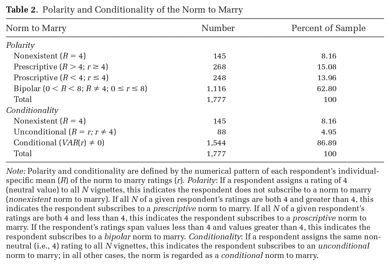
Note: Polarity and conditionality are defined by the numerical pattern of each respondent’s individual-specific mean (R) of the norm to marry ratings (r). Polarity: If a respondent assigns a rating of 4 (neutral value) to all N vignettes, this indicates the respondent does not subscribe to a norm to marry (nonexistent norm to marry). If all N of a given respondent’s ratings are both 4 and greater than 4, this indicates the respondent subscribes to a prescriptive norm to marry. If all N of a given respondent’s ratings are both 4 and less than 4, this indicates the respondent subscribes to a proscriptive norm to marry. If the respondent’s ratings span values less than 4 and values greater than 4, this indicates the respondent subscribes to a bipolar norm to marry. Conditionality: If a respondent assigns the same non-neutral (i.e., 4) rating to all N vignettes, this indicates the respondent subscribes to an unconditional norm to marry; in all other cases, the norm is regarded as a conditional norm to marry.
Conditionality of the norm to marry
Beyond the 62.80 percent of respondents who subscribed to a bipolar norm—which, by definition, is a conditional norm—24.09 percent of respondents subscribed to a conditional proscriptive norm or a conditional prescriptive norm, for a total of 86.89 percent. Altogether, the norm to marry in the United States is overwhelmingly conditional.
Intensity of the norm to marry
The norm to marry is intense among respondents who subscribed to an unconditional marriage norm, as they were relatively far from the neutral rating. For unconditional proscriptive norms (N = 33), the average distance (of the individual-specific mean ratings) from the neutral value is 3.24, and the average distance is 3.38 for unconditional prescriptive norms (N = 55). The small number of respondents (4.95 percent) who subscribed to an unconditional norm to marry favored extreme values, and the level of intensity is statistically equivalent for proscriptive and prescriptive norms, b = .139, SE = .203, p = .495. 11
Among conditional norms, the average distance is 1.72 for conditional proscriptive norms (N = 215) and 1.89 for conditional prescriptive norms (N = 213). The intensity of the norm to marry is statistically equivalent for respondents who subscribed to either a conditional proscriptive or prescriptive norm, b = .171, SE = .103, p = .100. 12 For individuals who subscribed to a bipolar marriage norm (N = 1,116), the average distance is 2.35, or moderately intense ratings.
The results show that the majority of the sample subscribes to a bipolar marriage norm where the average level of intensity is between “not very strong” and “somewhat strong.” Patterns in the data thus indicate that the overall intensity of the marriage norm is low-to-moderate.
Consensus about the norm to marry
The analysis of polarity, conditionality, and intensity indicates disagreement among respondents (see Appendix Figure A1 for histograms of individual-specific mean ratings of the norm to marry by norm type). To investigate consensus formally, we estimated the two-level HLMs outlined earlier. A likelihood ratio test rejected a model of fixed intercepts and slopes for each vignette dimension in favor of random intercepts and fixed slopes, χ2(1) = 4114.92, p < .001. In addition, we saw significant variation around the intercept as indicated by the level-2 error term, SD(intercept) = 1.427 (see Table 3, Model 1). This indicates differences across individuals in their tendencies to proscribe or prescribe marriage, thereby demonstrating respondent heterogeneity and a lack of normative consensus (Jasso 2006). 13
Next, we relaxed the assumption of fixed slopes, so that each respondent had a unique intercept and a unique slope for each vignette dimension. The results of a likelihood ratio test rejected a model of random intercepts and fixed slopes in favor of both random intercepts and random slopes, χ2(11) = 1134.83, p < .001. Stated differently, respondents differed with one another in their tendencies to proscribe or prescribe marriage and respondents placed different weights on the pecuniary and non-pecuniary circumstances demarcating the norm to marry. Thus, there is disagreement among respondents over the norm to marry.
Circumstances Demarcating the Norm to Marry
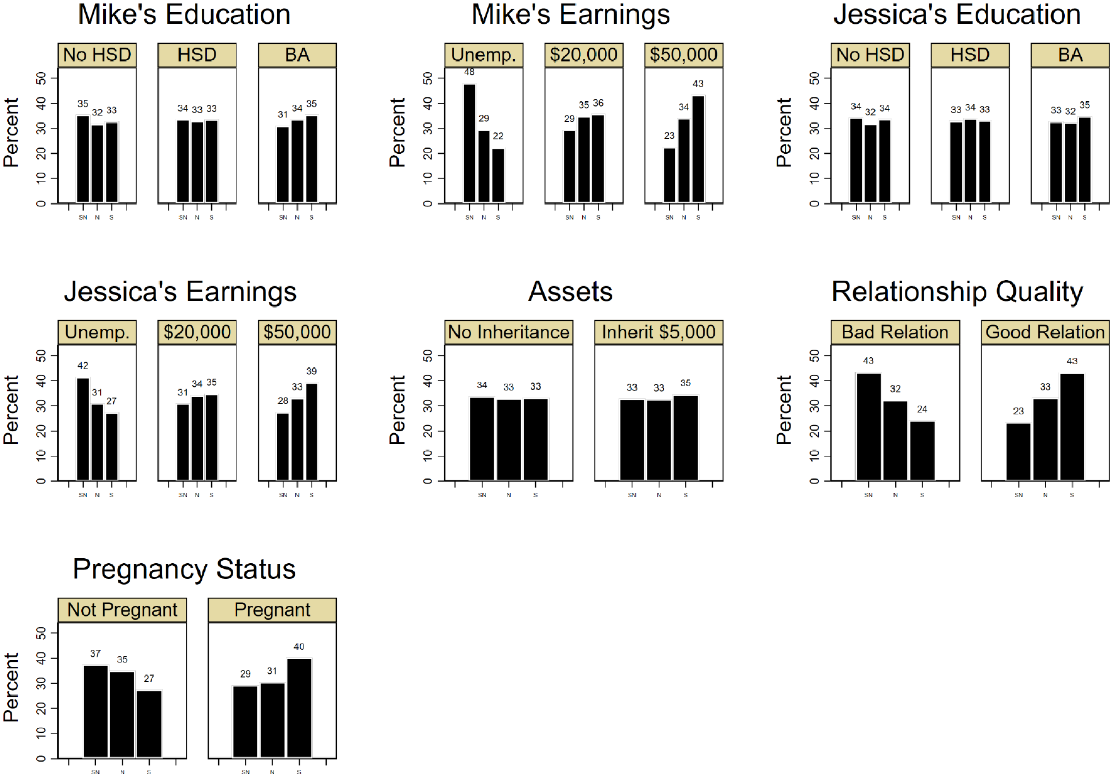
We now investigate respondents’ views about which circumstances demarcate, or serve as boundaries of, the norm to marry. We begin with a descriptive analysis that collapses the nine-point evaluation task into three categories: proscriptive (should not marry), nonexistent (neutral), and prescriptive (should marry). Figure 1 presents histograms of the distribution of the collapsed dependent variable by levels of each respective vignette dimension.
Histograms of the Norm to Marry by Vignette Dimensions
For education, the percentage of responses is roughly equivalent when either Mike or Jessica has no high school diploma or a high school diploma. However, 35 percent of responses—a plurality—prescribe marriage when either Mike or Jessica has a 4-year college degree. Mike and Jessica’s earnings produce slightly different, albeit expected, results. When Mike or Jessica is unemployed, a plurality of responses proscribe marriage (between 42 and 48 percent). But when Mike or Jessica is employed and earning money, the plurality switches from proscriptive to prescriptive, with the size of the plurality increasing as earnings increase. This shift is most noticeable for Mike’s earnings: only 23 percent of responses proscribe marriage when Mike earns $50,000 a year, whereas 43 percent prescribe marriage. Unlike education and earnings, assets generate only minor differences in the percentage of responses.
With respect to non-pecuniary circumstances, we see a shift from a plurality of responses proscribing marriage (43 percent) to a plurality of responses prescribing marriage (43 percent) as Mike and Jessica’s relationship quality goes from bad to good. Pregnancy status generates similar results. When Jessica is not pregnant, 37 percent of evaluations proscribe marriage. But when Jessica is pregnant, 40 percent of evaluations prescribe marriage. Overall, Figure 1 shows that responses vary dramatically between vignette dimensions and levels.
Table 3 presents results of two-level HLMs in which random slopes are fixed (Model 1) versus freely estimated (Model 2). In Model 1, we see strong statistical support for all seven vignette dimensions. The pecuniary circumstances (Mike and Jessica’s education, Mike and Jessica’s earnings and employment) affect views of marriage as expected: the greater education and earnings, the more prescriptive the norm to marry. Familywise tests of each dimension are statistically significant (see Table 3), as are pairwise tests between the second and third levels of each dimension (save for the second and third levels of Jessica’s education). Interestingly, the effect of earnings is not equal for Mike and Jessica. Mike’s earnings have stronger effects on the norm to marry than do Jessica’s earnings. Overall, our experimental design and sample finds evidence of an economic bar to marriage (Gibson-Davis et al. 2005; Gibson-Davis et al. 2018) that weighs men’s labor force characteristics more heavily than women’s (Gibson-Davis 2009; Smock et al. 2005).
Consensus and Conditionality of the Norm to Marry, Two-Level Hierarchical Linear Models
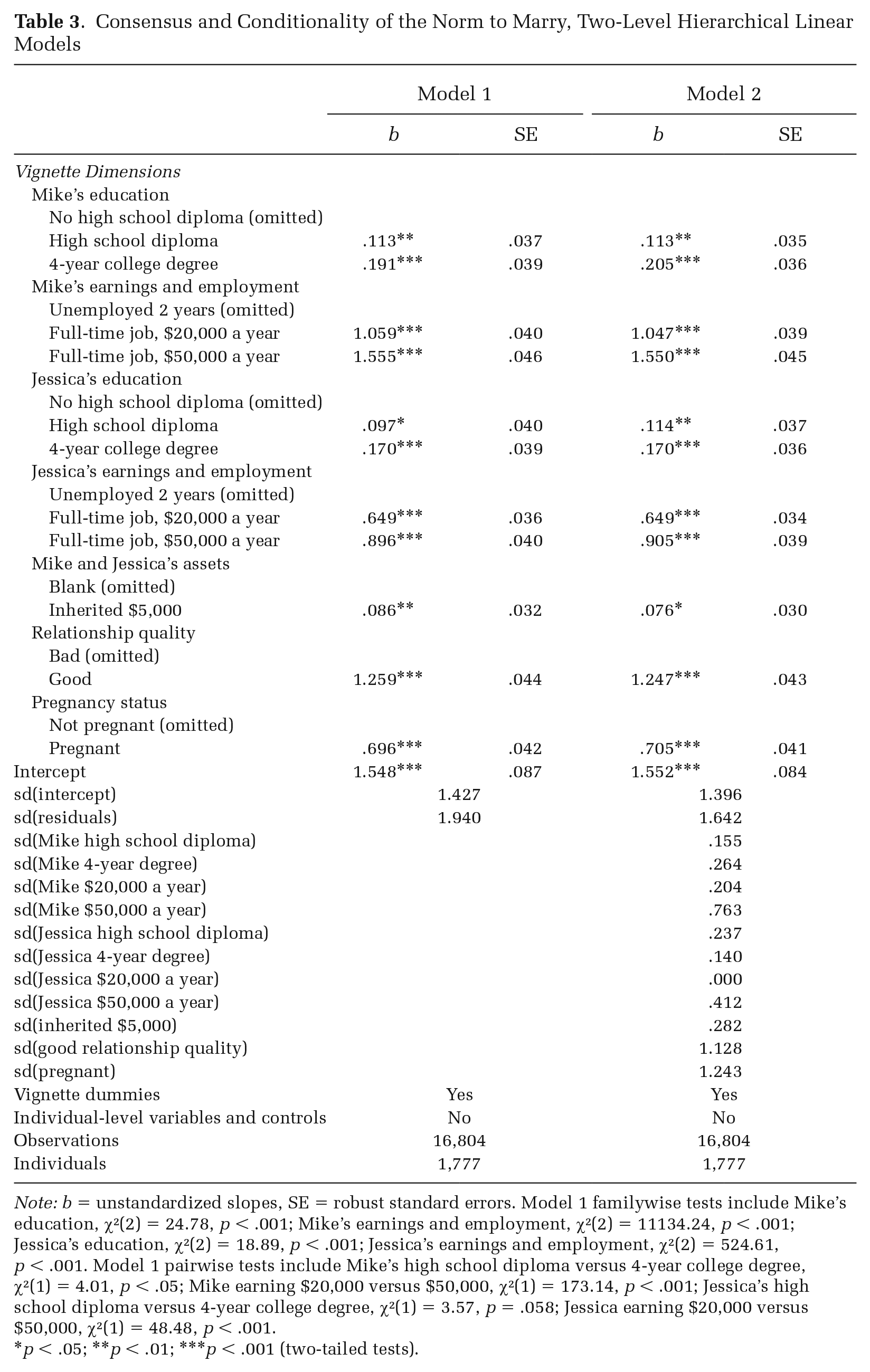
Note: b = unstandardized slopes, SE = robust standard errors. Model 1 familywise tests include Mike’s education, χ²(2) = 24.78, p < .001; Mike’s earnings and employment, χ²(2) = 11134.24, p < .001; Jessica’s education, χ²(2) = 18.89, p < .001; Jessica’s earnings and employment, χ²(2) = 524.61,p < .001. Model 1 pairwise tests include Mike’s high school diploma versus 4-year college degree,χ²(1) = 4.01, p < .05; Mike earning $20,000 versus $50,000, χ²(1) = 173.14, p < .001; Jessica’s high school diploma versus 4-year college degree, χ²(1) = 3.57, p = .058; Jessica earning $20,000 versus $50,000, χ²(1) = 48.48, p < .001.
p < .05; **p < .01; ***p < .001 (two-tailed tests).
The non-pecuniary circumstances in Model 1 yield similar dynamics: a pregnancy and a good quality relationship elicit stronger prescriptions to marry than no pregnancy or a bad quality relationship, respectively. In the contemporary United States, pregnancy continues to guide views about the necessity of marriage (Cherlin et al. 2008). Likewise, a bad quality relationship leads to opposition to marriage, likely due to beliefs about the futility of marriage (Wilcox and Nock 2006). Interestingly, relationship quality—as operationalized here—has a stronger effect on the norm to marry than does pregnancy. The higher-order needs of both individuals are thus more relevant to setting the norm’s boundaries than is a premarital conception.
Table 4 reports select linear predictions (and 95 percent CIs) by profiles of Mike and Jessica’s pecuniary (rows 1, 2, and 3) and non-pecuniary (columns 1 through 4) circumstances calculated from Table 3, Model 1 estimates. Starting with a low-economic-standing profile (i.e., Mike and Jessica do not have a high school diploma, are unemployed, and have no assets), respondents proscribe marriage between “not very strong” and “somewhat strong” (a linear prediction of 1.548) when Jessica is not pregnant and the quality of their relationship is bad. Only when Mike and Jessica achieve a moderate economic standing (i.e., both have a high school degree, earn $20,000 a year, and have assets) and are pregnant or have a good quality relationship do respondents prescribe marriage. Respondents prescribe marriage to the greatest extent—between “not very strong” and “somewhat strong” (a linear prediction of 6.405)—when Mike and Jessica achieve a high economic standing (i.e., both have a 4-year college degree, earn $50,000 a year, and have assets), when Jessica is pregnant, and when the quality of their relationship is good. Taken together, the linear predictions illustrate how strong the average treatment effects of the circumstances are in motivating respondents to proscribe or prescribe marriage.
Select Linear Predictions of the Norm to Marry
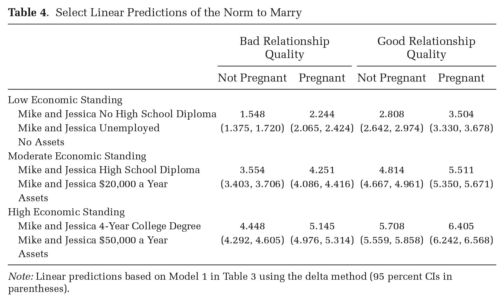
Note: Linear predictions based on Model 1 in Table 3 using the delta method (95 percent CIs in parentheses).
Returning to Table 3, we relax the assumption of fixed slopes in Model 2 to investigate which vignette dimensions vary in their magnitude. Of the pecuniary circumstances, only the effect of Mike earning $50,000 and Jessica earning $50,000 varies to a great extent between respondents (see Figure 2 for an illustration). There is generally consensus among respondents over the effects of Mike’s education, Jessica’s education, Mike earning $20,000, Jessica earning $20,000, and their shared assets on the norm to marry. In contrast, both pregnancy status and the quality of relationship vary to a great degree between respondents in their effects on the norm to marry. As Figure 2 shows, most respondents are prescriptive of marriage (to varying degrees) when Mike and Jessica are expecting a child; a small minority of respondents (roughly a quarter) are proscriptive of marriage under the same conditions. We see similar dynamics for the quality of Mike and Jessica’s relationship.
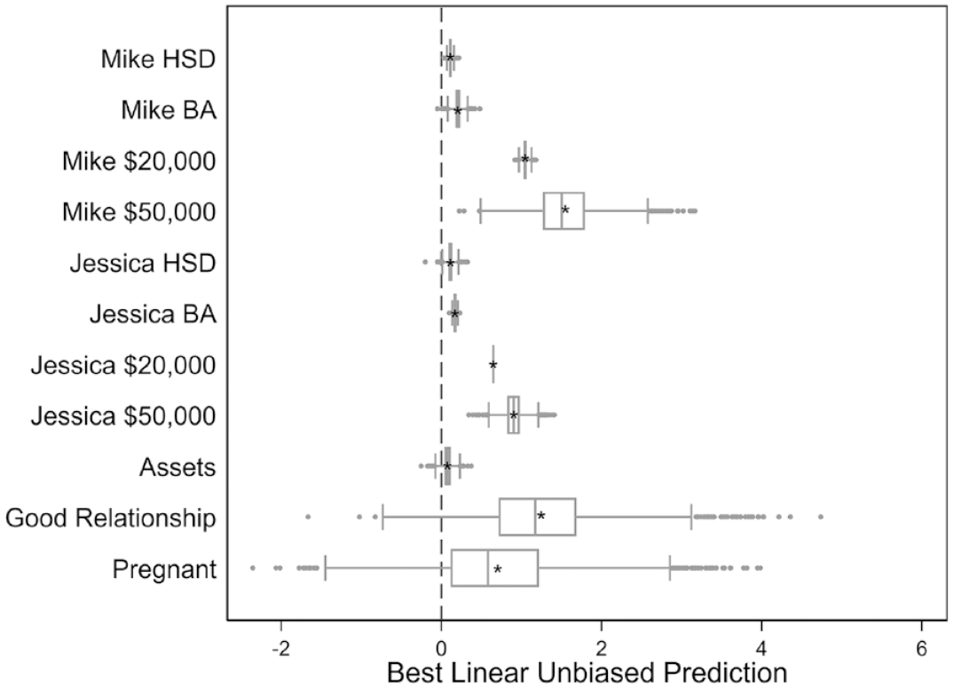
Boxplots of Best Linear Unbiased Predictions of Random Slopes
In short, both pecuniary and non-pecuniary circumstances serve as boundaries between who should and should not marry. Moreover, circumstances demarcating the norm to marry exhibit more consensus in some cases (education and assets) and less consensus in others (earnings, pregnancy status, and quality of relationship). Overall, however, we find relatively little consensus.
Consensus within and between Subpopulations: Race, Gender, and SES
In the next subsection, we identify whether individual-level tendencies to proscribe or prescribe marriage are a function of respondents’ race, gender, or SES. Then, we investigate whether variation in the weights placed on the circumstances driving the norm to marry is a function of respondents’ race, gender, or SES. 14
Character of the norm to marry within and between subpopulations
We now present estimates from a two-level HLM that includes respondents’ race, gender, and SES as predictors of normative differences. The model, in Table 5, controls for vignette dummies, vignette dimensions, and the individual-level control variables outlined in the Data and Methods section. These results show that White respondents and male respondents prescribe marriage more strongly than do Black respondents and female respondents, respectively. We see weak effects for SES: a familywise test for the effect of education is statistically non-significant, χ2(2) = 1.99 p > .10; the effect of income is statistically non-significant, b = –.070, SE = .040, p = .082; and a familywise test for the effect of occupational class is statistically non-significant, χ2(10) = 12.69, p > .10.
Consensus of the Norm to Marry across Subpopulations, Two-Level Hierarchical Linear Model
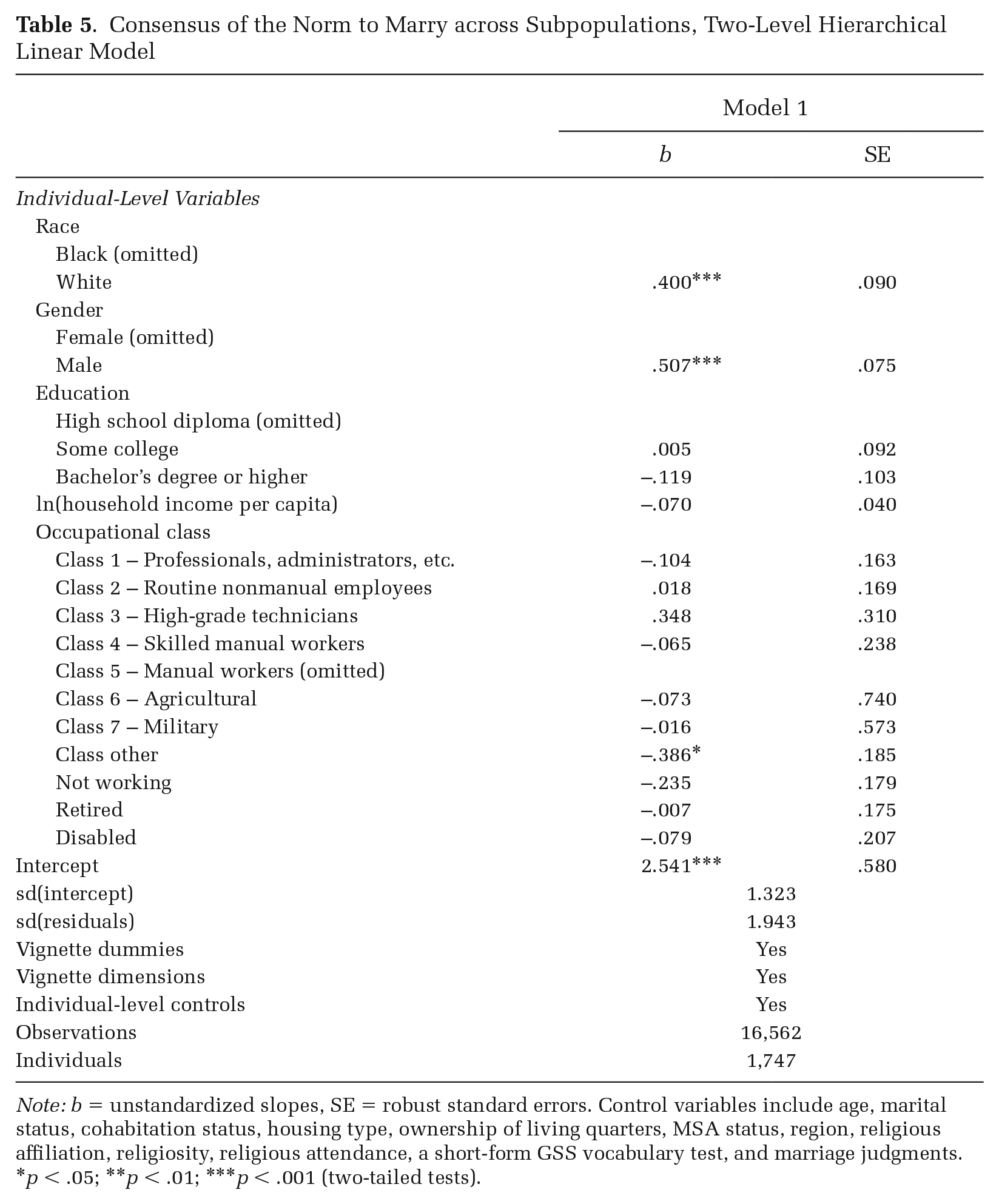
Note: b = unstandardized slopes, SE = robust standard errors. Control variables include age, marital status, cohabitation status, housing type, ownership of living quarters, MSA status, region, religious affiliation, religiosity, religious attendance, a short-form GSS vocabulary test, and marriage judgments.
p < .05; **p < .01; ***p < .001 (two-tailed tests).
Next, we investigate whether within-group variation is the same between subpopulations (e.g., consensus is greater or lesser among White respondents than among Black respondents). First, in Figure 3, kernel density plots of individual-specific mean ratings of the norm to marry reveal that the amount of disagreement (or lack of consensus) within subpopulations is comparable between subpopulations (e.g., disagreement among Black and White respondents is comparable). Second, tests of equality of variances across race, gender, and education yield statistically non-significant results, providing statistical support for the visualized patterns in Figure 3. 15 In short, male and female respondents, and Black and White respondents, differ in their tendencies to prescribe marriage, but the amount of disagreement (or lack of consensus) within groups is comparable between groups.
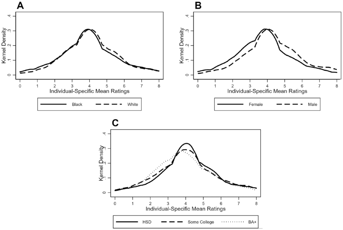
Kernel Density Plots of Individual-Specific Mean Ratings of the Norm to Marry by Race (Panel A), Gender (Panel B), and Education (Panel C)
Circumstances demarcating the norm to marry between subpopulations
Earlier, we found that some circumstances demarcating the norm to marry exhibit greater disagreement than others. We next investigate how much race, gender, and SES account for this disagreement by estimating a two-level HLM with cross-level moderation in which respondents’ race, gender, and education are interacted with each vignette dimension. 16 This model controls for vignette dummies, the individual-level control variables, and the other measures of SES (income and occupational class) outlined in the Data and Methods section. The model in Table 6 shows that the majority of cross-level interaction effects are statistically non-significant, and those that are statistically significant yield trivial substantive differences in the slopes (see Figures S1 and S2 in the online supplement). The two cross-level interaction effects that do yield practical and substantive differences are between race and quality of relationship as well as race and pregnancy status. The cross-level interaction effects show that the quality of relationship dimension has a stronger positive effect on the norm to marry for White respondents than for Black respondents (see Figure 4, panel A). The pregnancy status dimension has a weaker positive effect on the norm to marry for Black respondents than for White respondents (see Figure 4, panel B). Overall, we find evidence that Black and White respondents place different levels of importance on how relationship quality and pregnancy status affect the norm to marry. All other circumstances yield relatively consistent effects regardless of race, gender, or SES.
Consensus of Conditionality of the Norm to Marry across Subpopulations, Two-Level Hierarchical Linear Model with Higher Level Moderation of Lower-Level Effects
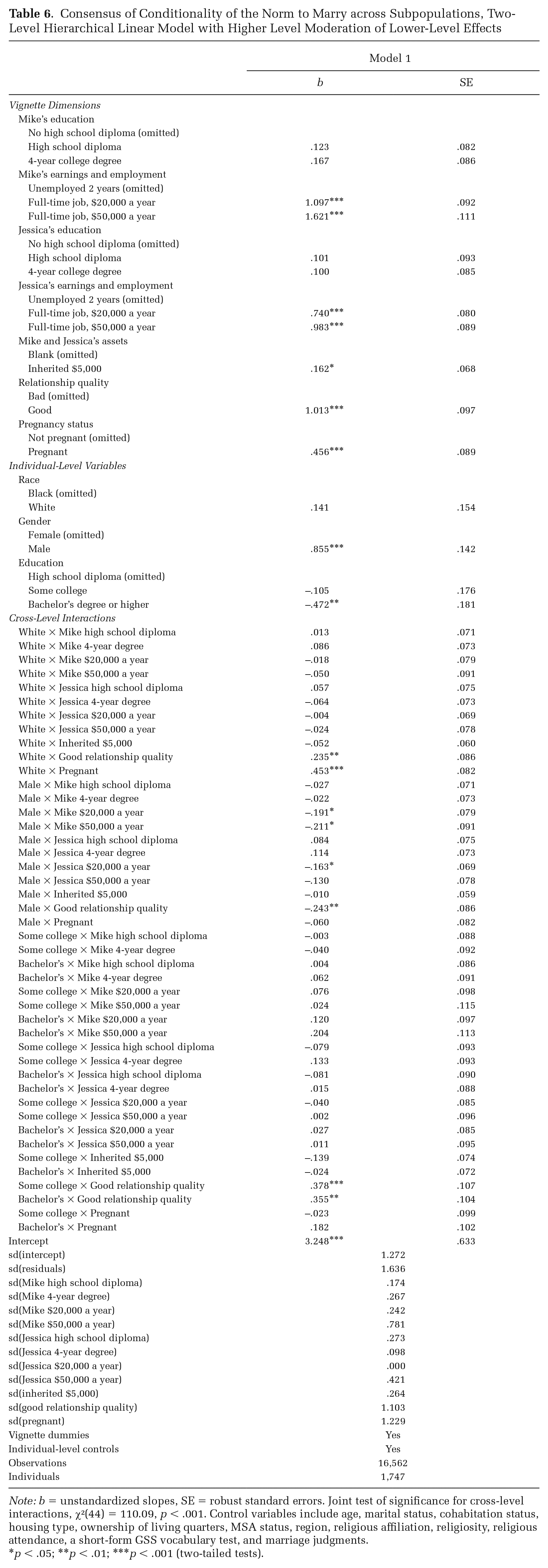
Note: b = unstandardized slopes, SE = robust standard errors. Joint test of significance for cross-level interactions, χ²(44) = 110.09, p < .001. Control variables include age, marital status, cohabitation status, housing type, ownership of living quarters, MSA status, region, religious affiliation, religiosity, religious attendance, a short-form GSS vocabulary test, and marriage judgments.
p < .05; **p < .01; ***p < .001 (two-tailed tests).
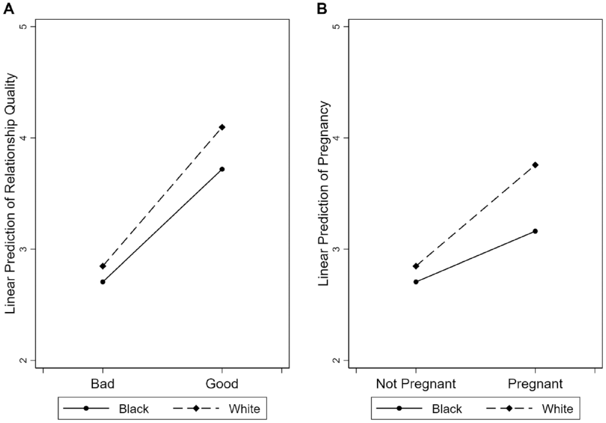
Cross-Level Interaction Effects between Race and Relationship Quality (Panel A) and Race and Pregnancy Status (Panel B) on the Norm to Marry (Table 6)
To provide a sense of the magnitude of disagreement across demographic groups, Table 7 reports select linear predictions (and 95 percent CIs) by the race and gender of respondents as well as Mike and Jessica’s non-pecuniary circumstances (estimates calculated from Model 1 in Table 6). When Jessica is not pregnant and the quality of Mike and Jessica’s relationship is bad, predicted values differ, at most, by 1 point (or a standardized mean difference of .379). 17 But when Jessica is pregnant and the quality of Mike and Jessica’s relationship is good, predicted values differ to a moderate extent, with Black females and White males, for instance, differing by 1.383 points (or a standardized mean difference of .526).
Select Linear Predictions of the Norm to Marry by Race and Gender
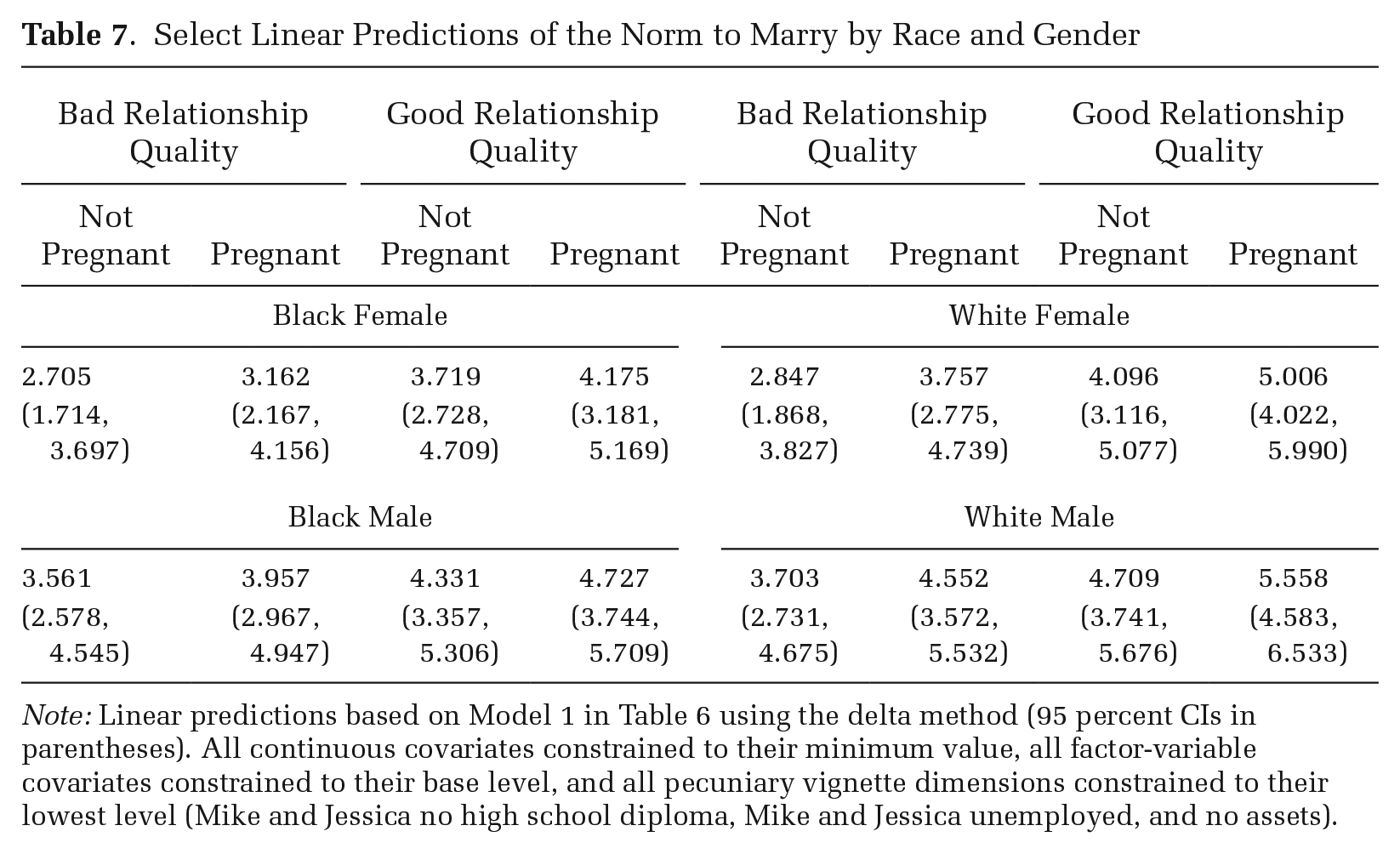
Note: Linear predictions based on Model 1 in Table 6 using the delta method (95 percent CIs in parentheses). All continuous covariates constrained to their minimum value, all factor-variable covariates constrained to their base level, and all pecuniary vignette dimensions constrained to their lowest level (Mike and Jessica no high school diploma, Mike and Jessica unemployed, and no assets).
Robustness and Sensitivity Checks
Robustness and sensitivity checks are in the online supplement. First, we estimated nested models with all possible higher-order interactions between vignette dimensions (e.g., two-way interactions, three-way interactions). According to the Bayesian information criterion, Model 1 in Table 3 is the best fitting model (Table S16). Second, characteristics of subpopulations may intersect in compelling ways to pattern norms about marriage in the United States. Poor Black Americans, for instance, exhibit different marriage patterns than do middle-class Black or White Americans (Raley et al. 2015). To investigate intersectionality, we estimated a series of models predicting random intercepts and random slopes by interacting respondents’ race, gender, and SES. Overall, models suggest that race, gender, and SES do not interact in complex (or consistent) ways to influence ratings of who should or should not marry (Tables S17 and S18). Third, the main effects are robust to alternative modeling procedures, namely two-level ordered logit (Tables S19 through S21) and multinomial logit regression (Tables S22 and S23). Fourth, the estimates are robust to models that exclude nonexistent norm followers (Tables S24 through S26) as well as models that restrict the analysis to respondents who evaluated all 10 vignettes (Tables S27 through S29). Fifth, we estimated all models found in the present manuscript using post-stratification survey weights provided by GfK (Tables S30 through S33). Weighted and unweighted models yield substantively similar results.
Discussion and Conclusions
The primary goal of the present study was to evaluate the strength of the norm about whether different-sex couples ought to marry in the contemporary United States. By turning our attention to the measurement of social norms within an experimental context, this article addresses a gap in our understanding of whether the norm to marry is weak or unevenly deinstitutionalized across race (Black, White), gender (male, female), or SES (education, income, and occupational class). In returning to our four original questions, we provide the following answers.
What Is the Character (Polarity, Intensity, Conditionality, Consensus) of the Norm to Marry among Black and White Americans in the United States, and What Does It Imply for the Deinstitutionalization of Marriage Thesis?
All four types of polarities—proscriptive, prescriptive, bipolar, and nonexistent—were observed in the sample, but the majority of respondents subscribed to a bipolar marriage norm, indicating that the norm to marry is overwhelmingly conditional. In terms of intensity, respondents’ overall magnitude of devotion to the marriage norm was low-to-moderate. Regarding consensus, individuals differed in their tendencies to proscribe or prescribe marriage, and they placed different weights on the circumstances governing marriage; thus, there is little consensus about the norm to marry.
Our results support Cherlin’s (2004:848) observation that “social norms [defining] people’s behavior in a social institution such as marriage” are weak in the United States. Despite this key finding, our results provide a nuanced picture of the contemporary institution of different-sex marriage: individuals still hold opinions about whether different-sex couples should or should not get married. Only a small minority of individuals are unwilling to state whether others should get married, suggesting a nonexistent norm. The remaining 92 percent of individuals subscribe to a norm, although the nature of the norm is conditional and does not exhibit consensus. Because different standards for action abound, these findings imply that individuals will be more prone to conflict, negotiation, and debate over who and why people should or should not get married (Cherlin 2004). This is what family scholars have observed in contemporary U.S. marriage for some time, as evidenced by debates over same-sex and interracial marriage (Powell et al. 2010). Yet, it remains to be seen whether more individuals in the United States will come to view the norm to marry as nonexistent and treat marriage as one of many possible family forms, driven by individual choices independent of what one (or others) should or should not do. Or, whether the norm to marry is in a transitional phase, moving from one normative system to another as it absorbs and layers on new types of unions—and represents new types of goals—under the umbrella of marriage.
What Are the Circumstances Demarcating, or Serving as Boundaries of, the Norm to Marry among Black and White Americans in the United States?
The majority of respondents subscribed to a conditional norm. One goal of the present study was to map the specific circumstances that predict variation in—or account for the conditionality of—the norm to marry. As expected, pecuniary and non-pecuniary circumstances act as the norm’s boundaries. The education and earnings of Mike and Jessica, their shared assets, as well as their pregnancy status and quality of relationship all drove respondents’ willingness to proscribe or prescribe marriage, with Mike’s earnings and employment having the strongest relative impact.
These findings align with Cherlin’s (2010:133) view of contemporary marriage in the United States, where marriage requires “a decent job, a good education, and the ability to attract a partner who is likely to treat you fairly, be loyal, and stay with you indefinitely.” Our findings support Cherlin’s view of marriage—but also add depth of understanding to the circumstances surrounding the institution of marriage—in two ways. First, we found that an economic bar is normative in the United States (Gassman-Pines et al. 2017; Gibson-Davis et al. 2018; Ishizuka 2018; Watson and McLanahan 2011), and men’s earnings (Mike) have stronger positive effects on attitudes toward different-sex marriage than do women’s earnings (Jessica) (Gibson-Davis 2009; Smock et al. 2005). Second, pregnancy status and relationship quality have dramatic effects on views of different-sex marriage in the United States (Cherlin et al. 2008; Gibson-Davis et al. 2016; Rackin and Gibson-Davis 2017; Waller and McLanahan 2005). When Mike and Jessica were expecting a child or when the quality of their relationship was good, the relative majority of responses prescribed marriage. The opposite occurred when Mike and Jessica were not pregnant or when their relationship quality was bad: the relative majority of responses proscribed marriage. In short, pregnancies and good quality relationships do engender beliefs that different-sex couples ought to marry, but economic considerations remain principal drivers of the approval of marriage. Still, some economic considerations, like education and assets, were of little practical significance. In the case of assets, this could be because the asset manipulation was relatively small, rather than because assets are unimportant: larger amounts of wealth may have proven more persuasive.
Are Individual Tendencies to Proscribe or Prescribe Marriage Universal or Specific to Subpopulations Based on Race (Black, White), Gender (Male, Female), or SES (Education, Income, Occupational Class)?
The tendency to proscribe or prescribe different-sex marriage was not universally shared. Instead, the (dis)approval of marriage was specific to particular subgroups. Race and gender have unique additive effects on tendencies to proscribe or prescribe marriage (with gender exhibiting a slightly larger effect than race), and SES was statistically unrelated to the norm to marry. Many of these findings support prior research. Women frequently report stronger negative attitudes toward marriage than do men (Sassler and Schoen 1999; Thornton and Young-DeMarco 2001)—which some argue is a function of sharp declines in the earning power of non-college-educated men coupled with gains in women’s economic self-sufficiency (Autor and Wasserman 2013)—and Black Americans are much less likely to marry than White Americans, and, when they do, it is at an older age (Raley et al. 2015; Tucker and Mitchell-Kernan 1995). Black Americans also harbor stronger negative attitudes toward marriage than do White Americans (South 1993). Nevertheless, our results diverge from this literature in two important respects.
First, individual tendencies to proscribe or prescribe marriage were different between Black and White respondents, but this effect was neither amplified nor dampened by gender. In other words, we did not find the Black-White difference among males was significantly larger or smaller than the difference among females. With additive inequalities, linear predictions yielded ratings for White males > Black males > White females > Black females. These inequalities, especially the difference between White males and Black females in attitudes toward different-sex marriage, have been observed in the literature (Wilcox and Wolfinger 2016), but they contradict prior Black-White gender differences in attitudes toward marriage (Bulcroft and Bulcroft 1993; South 1993).
Second, we discovered weak support for differences in the norm to marry across levels of SES. Individual tendencies to proscribe or prescribe marriage were similar regardless of respondents’ education, income, and occupational class. Yet, previous research finds that class is tightly coupled with marriage patterns and attitudes toward marriage (Daugherty and Copen 2016; Gubernskaya 2010; Kuo and Raley 2016; Raley et al. 2015; Torr 2011).
These seemingly conflicting findings can be reconciled by underscoring the SES of the focal couple and not the SES of respondents. We find that the economic conditions in which a specific marriage takes place demarcate who should and should not get married. Respondents, in other words, endorsed marriage to a greater extent when Mike and Jessica met an economic bar and achieved financial security prior to marriage. This observation was made possible because our experiment disentangled respondents’ SES from the financial and economic status of the couple under evaluation. Even more compelling, we found the effects of the economic bar and financial security on the norm to marry were the same regardless of the SES of respondents.
Are Circumstances Demarcating the Norm to Marry Universal or Specific to Subpopulations Based on Race (Black, White), Gender (Male, Female), or SES (Education, Income, Occupational Class)?
We found the effects of some circumstances varied statistically across respondents’ race, gender, and SES, but many effects were of small practical significance, save for Black-White differences in the effects of relationship quality and pregnancy status on the norm to marry. These results contribute to the literature in two important ways. First, our findings support the idea that Black-White differences in marriage patterns stem from compositional factors. Compositional arguments contend that marriage patterns differ between Black and White Americans because the pool of eligible partners is more constrained for Black Americans than for White Americans (Lichter et al. 1992; Schoen and Kluegal 1988; Wilson 1987), not because Black Americans place a greater emphasis on having economic supports in place prior to marriage than do White Americans (Bulcroft and Bulcroft 1993; Edin and Kefalas 2005). Our experiment reveals that Black and White respondents view economic resources similarly: Mike and Jessica’s education, earnings and employment, and assets affect prescriptions of marriage the same way regardless of respondents’ race or SES. It is not that Black respondents view the economic bar or financial status differently than White respondents, it is that Black respondents, on average, prescribe different-sex marriage to a lesser extent than do White respondents. We interpret this to mean that Black Americans may have—as Wilson (1987, 1996, 2009) contends—rejected marriage norms due to facing decades of institutional racism and economic dislocations unique to the Black population. In other words, economic and structural cleavages between Black and White Americans may have produced various cultural shifts, such as the deinstitutionalization of marriage in the Black community.
Second, we found that non-pecuniary circumstances demarcating the norm to marry did vary by respondents’ race and—to a lesser extent—SES. Although strongly positive for both racial groups, the effect of relationship quality on prescriptions of different-sex marriage was stronger for White respondents than for Black respondents. Qualitative and quantitative research shows that fears of infidelity and distrust of romantic partners is a common roadblock to marriage in the Black community (Anderson 1999; Carlson, McLanahan, and England 2004; Edin 2000; Edin and Kefalas 2005; Estacion and Cherlin 2010; Wilcox and Wolfinger 2016). Given these barriers, a potential interpretation of our findings is that Black Americans may be more skeptical of signifiers of relationship quality than White Americans. Like relationship quality, research finds Black-White differences in the relation between childbearing and marriage, with Black Americans less likely than White Americans to interpret pregnancy and childbearing as calling for marriage (Barber et al. 2015). Our study corroborates these findings: pregnancy status yields stronger prescriptions of marriage for White respondents than for Black respondents. The results, overall, buttress findings from the literature and lend experimental evidence in support of prior ethnographic observations.
Limitations and Directions for Future Research
Our research is not without limitations. First, future research should oversample individuals with less than a high school diploma. Cherlin (2020) distinguishes between non-college-educated and college-educated, but including respondents without a high school diploma is important given the rich ethnographic research probing views of marriage among individuals in extreme poverty who often drop-out or fail to complete their high school education (Edin and Kefalas 2005). Having respondents without a high school diploma would allow us to better generalize our results to those subpopulations, even though we observe variation on income and occupational class.
Second, future research should feature a comprehensive range of ethnoracial groups in the sampling frame. Research shows that Asian and Hispanic Americans exhibit different marriage and family patterns than do Black and White Americans (Raley et al. 2015). Hispanic Americans, for instance, have lower rates of marriage, higher rates of divorce, and higher rates of nonmarital childbearing than do White Americans (Cherlin 2020; Manning, Brown, and Stykes 2015; U.S. National Center for Health Statistics 2018). We chose to limit our sample to Black and White respondents given Cherlin’s (2004, 2020) focus on Black-White differences, but our FSE would yield compelling discoveries if administered to other ethnoracial groups. An application of our FSE to a representative sample of U.S. adults is a key goal for future research.
A third stream of research might extend our FSE to hypothetical different-sex and same-sex couples. A number of interesting questions could be addressed with this research: What is the character of the norm to marry for same-sex couples? Does the character of this norm vary by the gender of the couple? How does the character of the norm vary according to the sexual orientation of respondents? Research shows that attitudes toward same-sex marriage are changing in the United States but still exhibit divides along race, gender, SES, and especially religion (Powell et al. 2010). By addressing such questions with an FSE, we could experimentally test whether marriage as an institution has expanded to account for new types of romantic partnerships or has become increasingly obsolete in the face of same-sex unions.
Fourth, we investigated a limited number of circumstances demarcating the norm to marry, which may have affected estimates of conditionality and consensus. We did this to see whether people (dis)approve of different-sex marriage under commonplace marriage conditions and to offer a conservative test of the deinstitutionalization of marriage thesis, but other circumstances likely drive views of marriage. It would be useful for future research to investigate the impact of these alternative conditions. For instance, a number of other non-pecuniary circumstances might govern the norm to marry, including control over household decisions, fear of domestic violence, drug use, and multipartner fertility (Cherlin et al. 2008; Edin 2000; Edin and Kefalas 2005; Gibson-Davis et al. 2005; Smock et al. 2005; Waller 2002). Likewise, it would be beneficial to explore the bounds or limits of Mike’s and Jessica’s earnings and employment. We restricted our analysis to median incomes, but future FSEs should introduce and manipulate higher-income couples. Investigating the impact of these alternative conditions would supply further revelations about the character of the norm to marry.
Despite these limitations, our findings should be of interest to scholars broadly concerned with social norms and institutions. By crafting a novel FSE and using it to probe the character of norms about marriage, this research presents evidence on how measurement tools can shine new light on established areas of study—beyond collective action (Jasso and Opp 1997), bridewealth (Horne et al. 2018), and inequality (Rauhut and Winter 2010)—where institutions loom large as antecedent and consequent conditions. Following Cherlin’s (2020) recent theoretical considerations, we suggest future work focus on integrating the measurement of social norms with models of institutional change that underscore processes of institutional “layering” and “absorbing” (see Lauer and Yodanis 2010). This union between measurement and theory could fundamentally alter what we know about marriage and the family.
In conclusion, the present article extends our understanding of the deinstitutionalization of marriage by subjecting it—and other arguments found in the marriage and family literature—to gold standards of research: experimental methods and random samples. By using an FSE, the present article unearthed important observations about the increasingly stratified character of different-sex marriage in the United States (Cherlin 2020). We found that the norm about whether different-sex couples ought to marry is weak, that the norm varies across certain social groups, and that the relation between (non)pecuniary circumstances and views of marriage are causal. Future research can extend this work by tracking temporal variation in the norm to marry with an experimental design similar to our own. This would grant marriage and family scholars traction on the dynamics of deinstitutionalization. Researchers could follow trends in how the norm to marry is weakening: Is the norm becoming more bipolar, more conditional, less intense, or all three? Conversely, is the norm becoming more proscriptive or prescriptive, more unconditional, or more intense? The continued use of FSEs will help sociologists answer these sorts of questions.
Supplemental Material
sj-pdf-1-asr-10.1177_00031224221080960 – Supplemental material for Assessing the Deinstitutionalization of Marriage Thesis: An Experimental Test
Supplemental material, sj-pdf-1-asr-10.1177_00031224221080960 for Assessing the Deinstitutionalization of Marriage Thesis: An Experimental Test by Blaine G. Robbins, Aimée Dechter and Sabino Kornrich in American Sociological Review
Footnotes
Appendix
Summary Statistics and Descriptions of Individual-Level Variables
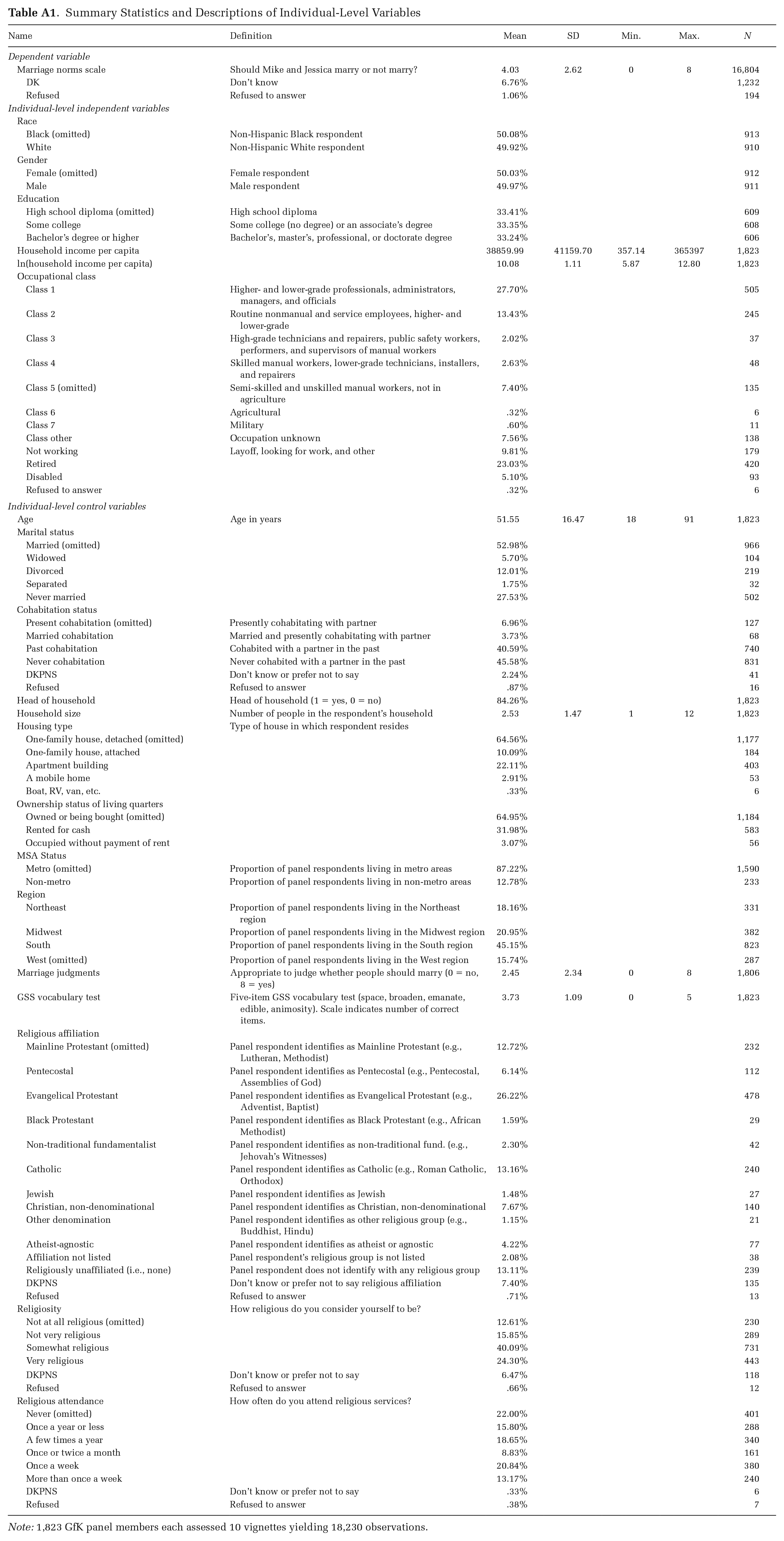
| Name | Definition | Mean | SD | Min. | Max. | N |
|---|---|---|---|---|---|---|
| Dependent variable | ||||||
| Marriage norms scale | Should Mike and Jessica marry or not marry? | 4.03 | 2.62 | 0 | 8 | 16,804 |
| DK | Don’t know | 6.76% | 1,232 | |||
| Refused | Refused to answer | 1.06% | 194 | |||
| Individual-level independent variables | ||||||
| Race | ||||||
| Black (omitted) | Non-Hispanic Black respondent | 50.08% | 913 | |||
| White | Non-Hispanic White respondent | 49.92% | 910 | |||
| Gender | ||||||
| Female (omitted) | Female respondent | 50.03% | 912 | |||
| Male | Male respondent | 49.97% | 911 | |||
| Education | ||||||
| High school diploma (omitted) | High school diploma | 33.41% | 609 | |||
| Some college | Some college (no degree) or an associate’s degree | 33.35% | 608 | |||
| Bachelor’s degree or higher | Bachelor’s, master’s, professional, or doctorate degree | 33.24% | 606 | |||
| Household income per capita | 38859.99 | 41159.70 | 357.14 | 365397 | 1,823 | |
| ln(household income per capita) | 10.08 | 1.11 | 5.87 | 12.80 | 1,823 | |
| Occupational class | ||||||
| Class 1 | Higher- and lower-grade professionals, administrators, managers, and officials | 27.70% | 505 | |||
| Class 2 | Routine nonmanual and service employees, higher- and lower-grade | 13.43% | 245 | |||
| Class 3 | High-grade technicians and repairers, public safety workers, performers, and supervisors of manual workers | 2.02% | 37 | |||
| Class 4 | Skilled manual workers, lower-grade technicians, installers, and repairers | 2.63% | 48 | |||
| Class 5 (omitted) | Semi-skilled and unskilled manual workers, not in agriculture | 7.40% | 135 | |||
| Class 6 | Agricultural | .32% | 6 | |||
| Class 7 | Military | .60% | 11 | |||
| Class other | Occupation unknown | 7.56% | 138 | |||
| Not working | Layoff, looking for work, and other | 9.81% | 179 | |||
| Retired | 23.03% | 420 | ||||
| Disabled | 5.10% | 93 | ||||
| Refused to answer | .32% | 6 | ||||
| Individual-level control variables | ||||||
| Age | Age in years | 51.55 | 16.47 | 18 | 91 | 1,823 |
| Marital status | ||||||
| Married (omitted) | 52.98% | 966 | ||||
| Widowed | 5.70% | 104 | ||||
| Divorced | 12.01% | 219 | ||||
| Separated | 1.75% | 32 | ||||
| Never married | 27.53% | 502 | ||||
| Cohabitation status | ||||||
| Present cohabitation (omitted) | Presently cohabitating with partner | 6.96% | 127 | |||
| Married cohabitation | Married and presently cohabitating with partner | 3.73% | 68 | |||
| Past cohabitation | Cohabited with a partner in the past | 40.59% | 740 | |||
| Never cohabitation | Never cohabited with a partner in the past | 45.58% | 831 | |||
| DKPNS | Don’t know or prefer not to say | 2.24% | 41 | |||
| Refused | Refused to answer | .87% | 16 | |||
| Head of household | Head of household (1 = yes, 0 = no) | 84.26% | 1,823 | |||
| Household size | Number of people in the respondent’s household | 2.53 | 1.47 | 1 | 12 | 1,823 |
| Housing type | Type of house in which respondent resides | |||||
| One-family house, detached (omitted) | 64.56% | 1,177 | ||||
| One-family house, attached | 10.09% | 184 | ||||
| Apartment building | 22.11% | 403 | ||||
| A mobile home | 2.91% | 53 | ||||
| Boat, RV, van, etc. | .33% | 6 | ||||
| Ownership status of living quarters | ||||||
| Owned or being bought (omitted) | 64.95% | 1,184 | ||||
| Rented for cash | 31.98% | 583 | ||||
| Occupied without payment of rent | 3.07% | 56 | ||||
| MSA Status | ||||||
| Metro (omitted) | Proportion of panel respondents living in metro areas | 87.22% | 1,590 | |||
| Non-metro | Proportion of panel respondents living in non-metro areas | 12.78% | 233 | |||
| Region | ||||||
| Northeast | Proportion of panel respondents living in the Northeast region | 18.16% | 331 | |||
| Midwest | Proportion of panel respondents living in the Midwest region | 20.95% | 382 | |||
| South | Proportion of panel respondents living in the South region | 45.15% | 823 | |||
| West (omitted) | Proportion of panel respondents living in the West region | 15.74% | 287 | |||
| Marriage judgments | Appropriate to judge whether people should marry (0 = no, 8 = yes) | 2.45 | 2.34 | 0 | 8 | 1,806 |
| GSS vocabulary test | Five-item GSS vocabulary test (space, broaden, emanate, edible, animosity). Scale indicates number of correct items. | 3.73 | 1.09 | 0 | 5 | 1,823 |
| Religious affiliation | ||||||
| Mainline Protestant (omitted) | Panel respondent identifies as Mainline Protestant (e.g., Lutheran, Methodist) | 12.72% | 232 | |||
| Pentecostal | Panel respondent identifies as Pentecostal (e.g., Pentecostal, Assemblies of God) | 6.14% | 112 | |||
| Evangelical Protestant | Panel respondent identifies as Evangelical Protestant (e.g., Adventist, Baptist) | 26.22% | 478 | |||
| Black Protestant | Panel respondent identifies as Black Protestant (e.g., African Methodist) | 1.59% | 29 | |||
| Non-traditional fundamentalist | Panel respondent identifies as non-traditional fund. (e.g., Jehovah’s Witnesses) | 2.30% | 42 | |||
| Catholic | Panel respondent identifies as Catholic (e.g., Roman Catholic, Orthodox) | 13.16% | 240 | |||
| Jewish | Panel respondent identifies as Jewish | 1.48% | 27 | |||
| Christian, non-denominational | Panel respondent identifies as Christian, non-denominational | 7.67% | 140 | |||
| Other denomination | Panel respondent identifies as other religious group (e.g., Buddhist, Hindu) | 1.15% | 21 | |||
| Atheist-agnostic | Panel respondent identifies as atheist or agnostic | 4.22% | 77 | |||
| Affiliation not listed | Panel respondent’s religious group is not listed | 2.08% | 38 | |||
| Religiously unaffiliated (i.e., none) | Panel respondent does not identify with any religious group | 13.11% | 239 | |||
| DKPNS | Don’t know or prefer not to say religious affiliation | 7.40% | 135 | |||
| Refused | Refused to answer | .71% | 13 | |||
| Religiosity | How religious do you consider yourself to be? | |||||
| Not at all religious (omitted) | 12.61% | 230 | ||||
| Not very religious | 15.85% | 289 | ||||
| Somewhat religious | 40.09% | 731 | ||||
| Very religious | 24.30% | 443 | ||||
| DKPNS | Don’t know or prefer not to say | 6.47% | 118 | |||
| Refused | Refused to answer | .66% | 12 | |||
| Religious attendance | How often do you attend religious services? | |||||
| Never (omitted) | 22.00% | 401 | ||||
| Once a year or less | 15.80% | 288 | ||||
| A few times a year | 18.65% | 340 | ||||
| Once or twice a month | 8.83% | 161 | ||||
| Once a week | 20.84% | 380 | ||||
| More than once a week | 13.17% | 240 | ||||
| DKPNS | Don’t know or prefer not to say | .33% | 6 | |||
| Refused | Refused to answer | .38% | 7 | |||
Note: 1,823 GfK panel members each assessed 10 vignettes yielding 18,230 observations.
Acknowledgements
We are indebted to Elisabeth Anderson, Paula England, Maria Grigoryeva, Edgar Kiser, Lake Lui, Ross Matsueda, John O’Brien, Michelle O’Brien, Karl-Dieter Opp, Steven Pfaff, Nora Schaeffer, Phi Su, three anonymous reviewers, and the editors of ASR for their advice and comments. We also benefited from the opportunity to present parts of this work to participants of the Social Research and Public Policy Writing Workshop at New York University Abu Dhabi, the workshop on The Future of Survey Experiments at New York University, and the 2020 Annual Meeting of the American Sociological Association. Finally, we would like to thank David Reisner and Magda Lasota from GfK for their research assistance.
Funding
This research was supported by a grant from the University of Washington’s Royalty Research Fund (A74643). Partial support for this research came from a Eunice Kennedy Shriver National Institute of Child Health and Human Development research infrastructure grant to the Center for Studies in Demography & Ecology at the University of Washington (R24 HD042828).
Notes
References
Supplementary Material
Please find the following supplemental material available below.
For Open Access articles published under a Creative Commons License, all supplemental material carries the same license as the article it is associated with.
For non-Open Access articles published, all supplemental material carries a non-exclusive license, and permission requests for re-use of supplemental material or any part of supplemental material shall be sent directly to the copyright owner as specified in the copyright notice associated with the article.