Data Processing Algorithm for Diagnostics of Combustion Using Diode Laser Absorption Spectrometry

Abstract

A new algorithm for the evaluation of the integral line intensity for inferring the correct value for the temperature of a hot zone in the diagnostic of combustion by absorption spectroscopy with diode lasers is proposed. The algorithm is based not on the fitting of the baseline (BL) but on the expansion of the experimental and simulated spectra in a series of orthogonal polynomials, subtracting of the first three components of the expansion from both the experimental and simulated spectra, and fitting the spectra thus modified. The algorithm is tested in the numerical experiment by the simulation of the absorption spectra using a spectroscopic database, the addition of white noise, and the parabolic BL. Such constructed absorption spectra are treated as experimental in further calculations. The theoretical absorption spectra were simulated with the parameters (temperature, total pressure, concentration of water vapor) close to the parameters used for simulation of the experimental data. Then, spectra were expanded in the series of orthogonal polynomials and first components were subtracted from both spectra. The value of the correct integral line intensities and hence the correct temperature evaluation were obtained by fitting of the thus modified experimental and simulated spectra. The dependence of the mean and standard deviation of the evaluation of the integral line intensity on the linewidth and the number of subtracted components (first two or three) were examined. The proposed algorithm provides a correct estimation of temperature with standard deviation better than 60 K (for T = 1000 K) for the line half-width up to 0.6 cm⁻¹. The proposed algorithm allows for obtaining the parameters of a hot zone without the fitting of usually unknown BL.

Keywords

Tunable diode laser absorption spectroscopy TDLAS combustion diagnostics data processing

Introduction

Diode laser absorption spectroscopy (DLAS) is widely used for diagnostics of temperature, concentration of molecular component, and total pressure in different hot zones of combustion in mixing gas flows.^1–4 The technique is based on fast scanning of the wavelength of a diode laser (DL) across the spectral range with the absorption lines of a test molecule. The detected absorption lines are then fitted with the theoretical spectra simulated using the spectroscopic databases like HITRAN,⁵ HITEMP,⁶ etc. In the fitting process, the searched parameters of a gas medium are used as the variables; their values are determined from the condition of the minimal residuals between the experimental and theoretical spectra. Temperature is inferred from the ratio of integral intensities of the two lines of a test molecule with different lower-state energy levels. The precision and accuracy of the temperature determination depend on the precision and accuracy of the integral line intensity evaluations which, in turn, depend on the experimental errors and algorithms of absorption spectra processing.

One of the crucial problems of DLAS is the fitting of the experimental lines. The difficulties of fitting are defined by high levels of noises in real propulsion, overlapping of different absorption lines of the test and foreign molecules and poor precision (in many cases) of the databases, especially for high temperatures and pressures. Different algorithms of data processing are used.^7–15 Mostly, individual absorption lines are fitted by Voigt profiles with Doppler widths, defined by the temperature, and different Lorentz widths. In some publications, contrary to the fitting of the individual line, simultaneous fitting of a part of the spectra with several lines are used.^11–14 This algorithm works well in case of low signal-to-noise (S/N) ratio when a weak line can be fitted with a large error.¹³

A big problem in the correct evaluation of the integral line's intensity is the correct evaluation of a BL in a real propulsion system. High levels of irregular acoustic and electric noises, interference effects, and so on distort the BL, thus reducing the precision of the integral intensity evaluation and, finally, the precision of line intensity ratio. Two approaches are used for data processing: stepwise and simultaneous. In most publications on DLAS applications, the stepwise approach is used.^10,15–17 The spectral zones without molecular absorption are selected and the BL is fitted using the polynomials. The problem of this algorithm is defined by the uncertainty of the selection of the spectral free zones. Mostly, due to the high spectral density of water lines in near-infrared (NIR), in close vicinity of the selected strong absorption lines of water, weaker lines are located. Their wings overlap strong lines and contribute in the integral profiles of the selected lines. This problem can be even more complicated because of the lines of the foreign molecules coexisting in the combustion zone. The broadening of the absorption lines in case of high pressure and temperature excludes the selection of a spectral interval within the fast scanning range of a DL free of any absorption.

In a simultaneous approach, the raw data are fitted by the theoretical absorption spectra and the BL simultaneously.^13,14 The BL is approximated usually by a polynomial of the degree not higher than 2. The coefficients of the polynomial and the line parameters are considered as the variables of the fitting.

The new algorithm of data processing in DLAS technique free of the fitting of a BL is developed in this paper.

Algorithms for Data Processing

In our previous publications,^12,13 the following algorithm was used. For the case of small absorption when the linear expansion of the Beer–Lambert formula is valid, the measurable absorption signal Y_i at the frequency ν_i can be presented in the form:

Y_{i} = \sum_{j} S_{j} (T) g_{j} (ν_{i} - ν_{0, j}) NL + b_{i} + ɛ_{i} = Z_{i} + b_{i} + ɛ_{i}

(1)

where S_j(T) is the integral intensity of the line j, g_j(ν_i – ν_0,j) is the line profile, N is the number density of the absorbing species, L is the length of the absorbing layer, Z_i is the theoretical absorption spectrum, ν_0j is the central frequency of the line j, b_i is the BL, and ɛ_i is the residual (difference between the experimental and simulated spectra). The BL in Eq. 1 was approximated by a polynomial b_i = Σk_nP_in, with k_n as the fitting variables and P_in – polynomial of the order n. A polynomial of order 2 or less was used. The intensity S_j(T) depends on temperature, the line profile depends on temperature and collisions. For the gas pressure of about 1 atm, the Voigt profiles are generally used for fitting.

At the first step, physically reasonable values of the initial concentration of absorbing species and temperature are selected, and using the nonlinear least squares method (NLSM),^18–20 the values of temperature and the concentration were found from the best fit of experimental spectra, e.g., from the minimal value of $\sqrt{< {ɛ_{i}}^{2} >}$ . In this algorithm simultaneous fitting of the simulated spectrum and BL (coefficients k_n) was used.

The idea of the new algorithm consists of the expansion of experimental Y_i and theoretical Z_i spectra (Eq. 1) in a series of orthogonal polynomials, subtracting of the first three components of the expansion from both the experimental Y_i and simulated Z_i spectra, and fitting the thus modified spectra. The BL is not fitted in this algorithm. Such an approach has the evident advantage of avoiding the fitting of the BL, which is very problematic in the case of strongly broadened lines when it is hardly possible to find the spectral points with zero absorption within the tuning range of a DL. Besides, the number of the variables is also reduced, which increases the robustness of the fitting process.

The scheme of the new algorithm consists of several steps.

1. The set of the orthogonal polynomials^21,22 is formed. In our case, the polynomials P_in are defined as the orthogonal at the manifold of points i (1 ≤ i ≤ K), if they satisfy the relation

\sum_{i = 1}^{K} P_{in} P_{im} = δ_{nm}

(2)

The set of such polynomials can be constructed using the recurrence relation

λ_{n} P_{i, n + 1} = (i - a_{n}) P_{i, n} + b_{n} P_{i, n - 1}

(3)

where the coefficients

\begin{matrix} a_{n} = \sum_{i = 1}^{K} {iP}_{in}^{2} \\ b_{n} = \sum_{i = 1}^{K} i P_{in} P_{i, n - 1} \end{matrix}

(4)

λ_n are defined from normalization condition. Calculation of the coefficients is started with the conditions:

\begin{matrix} P_{i, - 1} \equiv 0 \\ P_{i, 0} = K^{- 1 / 2} \end{matrix}

(5)

This approach is a simplified version of more general case described by Forsythe²¹ and Hudson.²² In our version we use equidistant points i instead of x_i used by Hudson.²²

At the next step, both experimental Y_i (Eq.1) and theoretical Z_i (Eq.1) spectra are expanded in the manifold of the orthogonal polynomials P_i

\begin{matrix} Y_{i} = \sum_{n = 0}^{K - 1} α_{n} P_{in} \\ Z_{i} = \sum_{n = 0}^{K - 1} η_{n} P_{in} \end{matrix}

(6)

where the coefficients are determined as

α_{n} = \sum_{i = 1}^{K} Y_{i} P_{in}

η_{n} = \sum_{i = 1}^{K} Z_{i} P_{in}

Then the first three components of the expansion on the orthogonal polynomials are subtracted from the experimental Y_i and theoretical Z_i spectra; thus, the modified experimental Y_mod,i and theoretical Z_mod,i spectra take the form:

\begin{matrix} Y_{mod, i} = Y_{i} - \sum_{n = 0}^{2} α_{n} P_{in} \\ Z_{mod, i} = Z_{i} - \sum_{n = 0}^{2} η_{n} P_{in} \end{matrix}

(7)

Finally, the reduced experimental spectrum Y_mod is fitted by the reduced theoretical one Z_mod using the NLSM with the criteria of minimal residual:

\sum_{i = 1}^{N} {(Y_{mod, i} - Z_{mod, i})}^{2} = \sum_{n = 3}^{N - 1} {(α_{n} - η_{n})}^{2} \to min

(8)

Example of the New Algorithm Application

It is noteworthy that in the experiments on propulsion systems one never knows the actual temperature because there is no independent trustworthy technique like thermocouple or pyrometer. Thus, only numerical experiments can test the correctness of an algorithm.

The operation of the new algorithm will be demonstrated by a simulation of the theoretical spectra H₂O, the addition of an arbitrary BL, and white noise and fitting of such constructed experimental spectrum using the new algorithm. For temperature evaluation, two spectral intervals were processed: 7183–7186 cm⁻¹ and 7443–7446 cm⁻¹. These intervals were selected as the optimal ones for the temperature range up to 2000 K and total pressure up to 3 atm.²³ The algorithm was applied for both intervals simultaneously. The details of the algorithm operation will be demonstrated for the first interval.

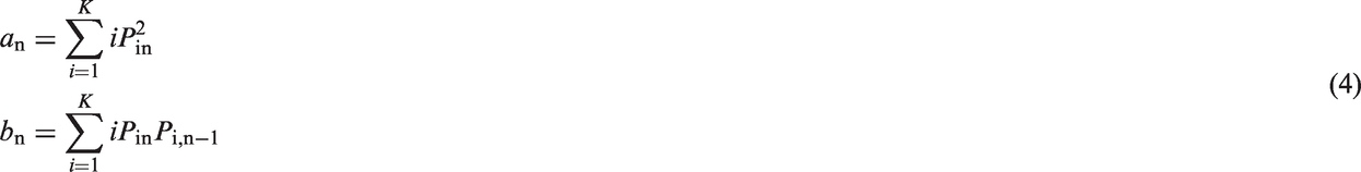
Nine panels are presented in Fig. 1. In panel 1, the fragment of H₂O spectrum with the strong line 7185 cm⁻¹ is shown. The spectrum is simulated for the temperature 1000 K, total pressure 3 atm, and water molar fraction 1%. All water lines with the intensities above 1% of the strong line intensity were used for simulation. The position of the line centers, intensities, and line broadening coefficients were taken from HITRAN2012.⁵ The BL in the form of the quadratic polynomial and white noise (the mean noise density of 6% of the 7185 cm⁻¹ line amplitude) are added to the simulated spectrum. The coefficients k_n of the polynomial were selected to simulate the BL in the manner of the actual one registered in our previous experiments²³ (k₀ = 0.01, k₁ = 0.02, k₂ = 0.005).

Figure 1.

Results of the numerical experiments. Panel 1 shows the fragment of H₂O spectrum with the strong line 7185 cm⁻¹. Panel 2 shows the sum of three first polynomials, calculated for the data of panel 1. Panel 3 shows the modified experimental spectrum - the difference between panels 1 and 2. The second row, panels 4, 5, and 6, shows the same sequence of the spectra but for the seed spectrum (Z). Panel 7 presents the best theoretical absorption spectrum. Panel 8 shows the calculated sum of the first three polynomials for spectrum 7. Panel 9 shows the best fit of the modified theoretical spectrum to the modified “experimental” one (panel 3) and the minimal residuals. See further explanations in the text.

Panel 2 shows the sum of three first components ( $\sum_{n = 0}^{2} α_{n} P_{in}$ ), calculated for the data Y_i of panel 1. Panel 3 shows the modified experimental spectrum Y_mod,i , the difference between Y_i and ( $\sum_{n = 0}^{2} α_{n} P_{in}$ ).

The second row in Fig. 1 presents the same sequence of the panels, but for the seed spectrum Z. This spectrum was simulated for the set of parameters (temperature, H₂O concentration, optical length, the width of the Lorentz part of the Voigt profile) to be expected in real experiments. Panel 4 shows pure seed spectrum Z_i (without BL and noise) for the temperature 900 K and pressure 2 atm and water molar fraction 1%. The sum of three components $\sum_{n = 0}^{2} η_{n} P_{in}$ of expansion of Z_i in a series of orthogonal polynomials is presented in panel 5, while the difference between panels 4 and 5 (Z_mod,i) is shown in panel 6.

After the simulation of the experimental and theoretical spectra, fitting of these modified spectra is started. In the fitting procedure, each line used for the construction of the spectra is approximated by the Voigt profile. The independent fitting variables are temperature, water concentration, the position of the strong lines, and independent Lorentz linewidths. The positions of the weak lines are fixed relative to the strong lines according to HITRAN2012.⁵ Small shifts of the weak lines with a variation of the temperature were neglected. The temperature is determined as the result of the fitting in two spectral ranges around 7185 and 7444 cm⁻¹.

At each iteration step, a new theoretical spectrum Z_i with a new set of parameters is simulated, new sum $\sum_{n = 0}^{2} η_{n} P_{in}$ is calculated, the resulting Z_mod,i is constructed and compared with the modified experimental spectrum Y_mod,i (panel 3). The procedure continues until a minimal squared residual (Eq. 8) is achieved. The results of the fitting are shown in the panels 7–9. Panel 7 presents the best theoretical absorption spectrum. Panel 8 shows the calculated sum $\sum_{n = 0}^{2} η_{n} P_{in}$ for this spectrum 7, while panel 9 shows the best fit of the modified theoretical spectrum to the modified experimental one (panel 3). The minimal residuals are also presented in panel 9.

This fitting procedure was repeated for each of 100 realizations of the noise. The mean temperature estimated by the new algorithm from 100 realizations was 1014 K, standard deviation sd(T) was 60 К.

Dependence of the Precision and Accuracy of the Hot Zone Parameters Evaluation on the Linewidth

The dependence of the efficiency of the proposed algorithm on the widths of the absorption lines will be discussed in more details in this section. The performance of the algorithm is based on the removing of the first three components of the orthogonal polynomial expansion of the experimental spectrum. The functioning of the algorithm will be demonstrated by the processing of a single absorption line located in the center of the 3 cm⁻¹ tuning range of a DL. The prime goal of these studies is the dependence of the metrological parameters on the linewidth. The position of the line was located in the center of a DL tuning range just to simplify calculations and clarify the results. In addition, by tuning the parameters of a DL (temperature, current) one can locate the line in the center of the tuning range.

Figure 2 shows three Voigt profiles with different widths and BL. These profiles were simulated with equal Doppler halfwidth 0.019 cm⁻¹ and Lorentz halfwidths 0.02 (panel 1), 0.16 (panel 3), and 0.32 cm⁻¹ (panel 5). The selected Doppler halfwidth corresponds to 1000 K. The BL was approximated by a parabola with the projections on the orthogonal polynomials α₀ = 0.02, α₁ = 0.02, and α₂ = 0.02. In the calculations, the partial pressure of the water vapor was assumed equal to 1% of the total gas pressure. In simulations, the total pressure was assumed to be 1 atm in panel 1, 8 atm in panel 3, and 16 atm in panel 5. For all spectra the optical absorption length L was assumed as 10 cm, and S₀ = 5 × 10⁻²¹ cm/mol.

Figure 2.

Simulated absorption spectra for different linewidth (left panels 1, 3, 5) and the amplitudes of the projections of the corresponding spectra on the orthogonal polynomials (right panels 2, 4, 6). The profiles are simulated for equal Doppler half-width 0.019 cm⁻¹ and Lorentz half-widths 0.02 (panel 1), 0.16 (panel 3), and 0.32 cm⁻¹ (panel 5). The BL was approximated by a parabola. Panels 2, 4, and 6 present the amplitudes of the projections of spectra (panels 1, 3, 5) on the orthogonal polynomials. The projections of the profiles are presented in black and the projections of the BL are shown in gray.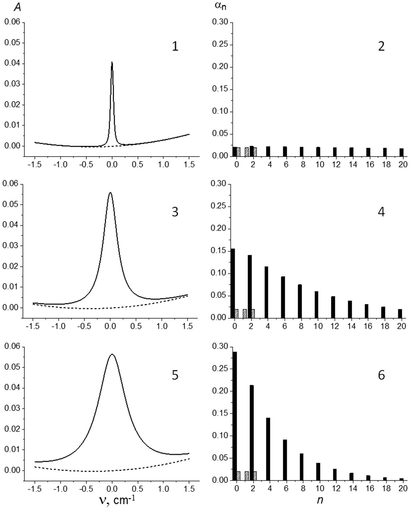

Panels 2, 4, and 6 in Fig. 2 present the amplitudes of the projections of these spectra (panels 1, 3, 5) on the orthogonal polynomials. The projections of the profiles are presented in black and the projections of the BL are shown in gray.

In Fig. 2 (panels 2, 4, 6) the numbers in the abscissa axes present the order of the orthogonal polynomials (from 0 to 20); the ordinate presents the amplitude of the absorption line projections on the polynomials (α_n). The figure shows the decrease in the number of the essential components in the expansion with the increase of the linewidth. Noteworthy, due to the location of the lines in the center of the spectral range, the odd components are absent because in this case line profiles are symmetrical.

The described procedure of the spectrum reduction means the subtraction of the first three components in the expansion. The results in Fig. 2 show that the broader the linewidth, the greater the part of the absorption line, which contributes to the first three components in the expansion. In other words, the broader the line, the larger the part of the absorption line subtracted according to the algorithm, which evidently increases the standard deviation in the evaluation of the integral intensity, which in turn increases the error in temperature evaluation. Below the dependence of the accuracy and precision of the temperature evaluation on the linewidth will be examined.

The standard deviation of the temperature evaluation depends on the errors in the line intensities estimation in the form:^13,23

sd (T) = \frac{T^{2}}{T_{eff}} (\frac{{(sd (S_{1}))}^{2}}{{(S_{1})}^{2}} + \frac{{(sd (S_{2}))}^{2}}{{(S_{2})}^{2}})^{1 / 2}

(9)

where

T_{eff} = \frac{hc Δ E ″}{k}

, ΔE^″ is the energy difference between the lower-state levels of the transitions 1, 2 are used for temperature estimation, sd(S_i) are standard deviations of the line integral intensities S_i.

Furthermore, it is the error of the integral intensity estimation that will be examined in detail because this error defines the one of the temperature estimation (Eq. 9). In calculations, the profiles presented in Fig. 2 (left panels) were modified by the addition of white noise with σ = 10⁻³ (about 2% of the line amplitude).

The step-by-step processing of the calculations of dependences of the mean line intensity and standard deviation on the linewidth looks as follows:

The line with Voigt profile is constructed and the BL is added;

100 realizations of white noise are then added to the constructed spectra;

Mean integral intensity and sd(S) are calculated;

This procedure is realized for variable Lorentz parts of Voigt profile; at each step of the spectra simulation the Lorentz halfwidth was increased by √2 times from 0.02 to 0.7 cm⁻¹ (as in previous simulations the partial pressure of the water vapor was assumed to be equal to 1% of the total gas pressure);

The new algorithm of the experimental and simulated spectra reduction is realized for two cases – subtraction of the first two components and the three ones.

The results of the numerical experiments are presented in Fig. 3. The dependence of the mean integral intensity $\bar{S}$ and relative standard deviation rsd(S) = sd(S)/S₀ on the linewidth are shown.

Figure 3.

Dependence of the relative standard deviation rsd (S): (a) and relative mean integral intensity 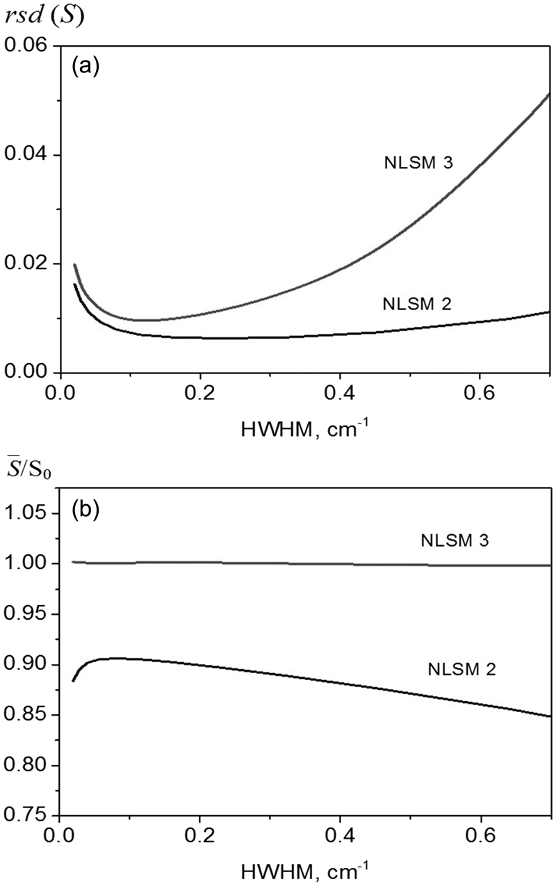$\bar{S}$ /S₀; (b) on the line half-width. S₀ = 5 × 10⁻²¹ cm/mol was used in simulations of the “experimental” spectra.

Figure 3a shows the dependences of the rsd(S) on the line half-width at half maximum (HWHM) for subtraction of two (NLSM 2) and three (NLSM 3) first components from the “experimental” and simulated spectra. Figure 3b presents the same dependences of the mean integral intensities $\bar{S}$ for two cases. Evidently, the rsd(S) for the subtraction of only two projections is lower than the rsd(S) for the subtraction of all three projections within the whole investigated linewidth range. As was mentioned above, such behavior can be explained by a larger part of the profile which is subtracted in the case of NLSM 3.

At the same time, the mean values $\bar{S}$ are estimated correctly if three projections are subtracted (Fig. 3b). The $\bar{S}$ for the case of subtraction of only two projections gives the underestimation of the correct value S₀ more than 10%, while the correct value S₀ for $\bar{S}$ is calculated by the subtraction of the first three components. It can be explained by the specific behavior of the BL in our numerical experiment. The BL was constructed in the form of a parabola; thus, the subtraction of only two components results in an incomplete elimination of the BL, while the subtraction of three components results in the correct estimation of the integral intensity.

Figure 3a shows that the standard deviation grows for the line HWHM above 0.2 cm⁻¹. At the same time, the growth is not very dramatic, as for the line HWHM 0.6 cm⁻¹ the rsd(S) is only 4%. It is noteworthy that these values were estimated for relatively low white noise (2% of the line amplitude).

The estimation of the errors of temperature evaluation based on the rsd(S) can be obtained using Eq. 9. For the line HWHM 0.02 cm⁻¹ (Fig. 2, panel 1), the rsd(S) is about 0.02 (Fig. 3a). Assuming equal rsd(S) for both lines, the value sd(T) is estimated at 30 K. For the line HWHM 0.2 cm⁻¹, the rsd(S) is about 0.015, which results in sd(T) about 20 K. For the line HWHM 0.6 cm⁻¹ sd(T) is about 60 K.

In these calculations, the temperature of 1000 K was used for simulation of the “experimental” line. The results in Fig. 3b show that subtraction of the first three components provides precise determination of the temperature ( $\bar{S}$ /S₀ ≈ 1). The subtraction of only two components provides a bias of the temperature ΔT from the postulated one to 120 K for the width 0.02 cm⁻¹, 100 K for the width 0.2 cm⁻¹ and 140 K for the width 0.6 cm⁻¹.

Example of the Real Experimental Absorption Spectra Processing

The use of the developed algorithm will be exemplified by processing the H₂O molecule absorption spectra registered in the experiments on the real propulsion system in the Zhukovskii Aerodynamic Institute. A detailed description of the experimental setup and the measurements technique are presented elsewhere.²⁴ Only brief information is given below.

Two pig-tailed DFB DLs (Sacher Lasertechnik) generating in spectral ranges of 7185 cm⁻¹ (λ = 1.392 µm) and 7444 cm⁻¹ (λ = 1.343 µm) were used in the experimental DLAS spectrometer. The outputs of both DLs were coupled by a multiplexer in the single-mode optical fibers and transmitted to the propulsion system. The fiber was about 30 m long, enabling allocation of the sensitive parts of the spectrometer in a separate room away from the experimental complex.

Two sapphire windows on the opposite sides of the test camera were installed for input and output of the probing laser beam. The mixing flows of air and oxidant were preheated to a variable temperature in a separate chamber located before the test camera. Temperature and total flow pressure could be changed by varying the temperature in the preheating chamber and by inserting a throttle in the flow (either mechanical or a gas cross-flow). In the experiments, the temperature in the flow varied in the range of 600–1900 K and pressure was within the range of 0.6–3 atm. Depending on the temperature in the preheating chamber, partial concentration of water vapor was in the range of 3–8%.

A single run of the process started with the heating of air in the chamber to a certain temperature, then the mechanical valve was opened and hot air (temperature about 700 K) expanded into the combustion camera. At a certain moment, the throttle was switched on and the temperature and pressure in the flow increased. The process lasted 3–5 s.

During the whole run, both DLs were on and the absorption spectra were registered during about 5 s. One scan of data collection was 40 ms, with 20 ms scan of each DL across the tuning range ∼3 cm⁻¹. Data processing was performed on-line and off-line.²⁴

The experimental spectra and the results of data processing using the developed algorithm are shown in Fig. 4. Real experimental raw spectra registered in one scan, i.e., when the total pressure increased to 3 atm, are presented in Fig. 4 (upper row). The results of the fitting are shown in the middle row. As described, experimental and theoretical spectra were modified by subtraction of the first three components of their polynomial expansion. Theoretical spectra were obtained using the HITRAN database.⁵ In a previous publication,³ we examined the dependence of the accuracy of the temperature evaluation on the number of the absorption lines included in the simulations. We used two lines for the range 7185 cm⁻¹ and four lines for the range 7444 cm⁻¹. The general result was evident: if more lines are included, a better fitting can be done. In the present paper, we used 16 lines for the first spectral range and 19 lines for the second one. The residuals resulting from the fitting of the modified spectra are shown in Fig. 4 in the bottom row. The results prove the adequate fitting of the experimental spectra. The temperature evaluated in this run using the developed algorithm was 1165 K. The same spectra were processed using the “standard” algorithm of simultaneous fitting of the spectra and the BLs. The calculated temperature was essentially similar: 1160 K. In our opinion, such a minimal difference can be explained by a relatively high S/N ratio in the spectra in Fig. 4. In the case of weaker line intensities, the developed algorithm will be more adequate. The computation time of these spectra processing for the developed algorithm is about half that of the algorithm for simultaneous fitting.

Figure 4.

Experimental absorption spectra and the results of fitting. The raw spectra in the vicinity of 7185 cm⁻¹ (left) and 7444 cm⁻¹ (right) are shown in the top row. The results of fitting with subtraction of the first three components from the spectra and the BLs are shown in the middle row (experimental spectra in black, simulated spectra in gray shadow). The residuals are shown in the bottom row.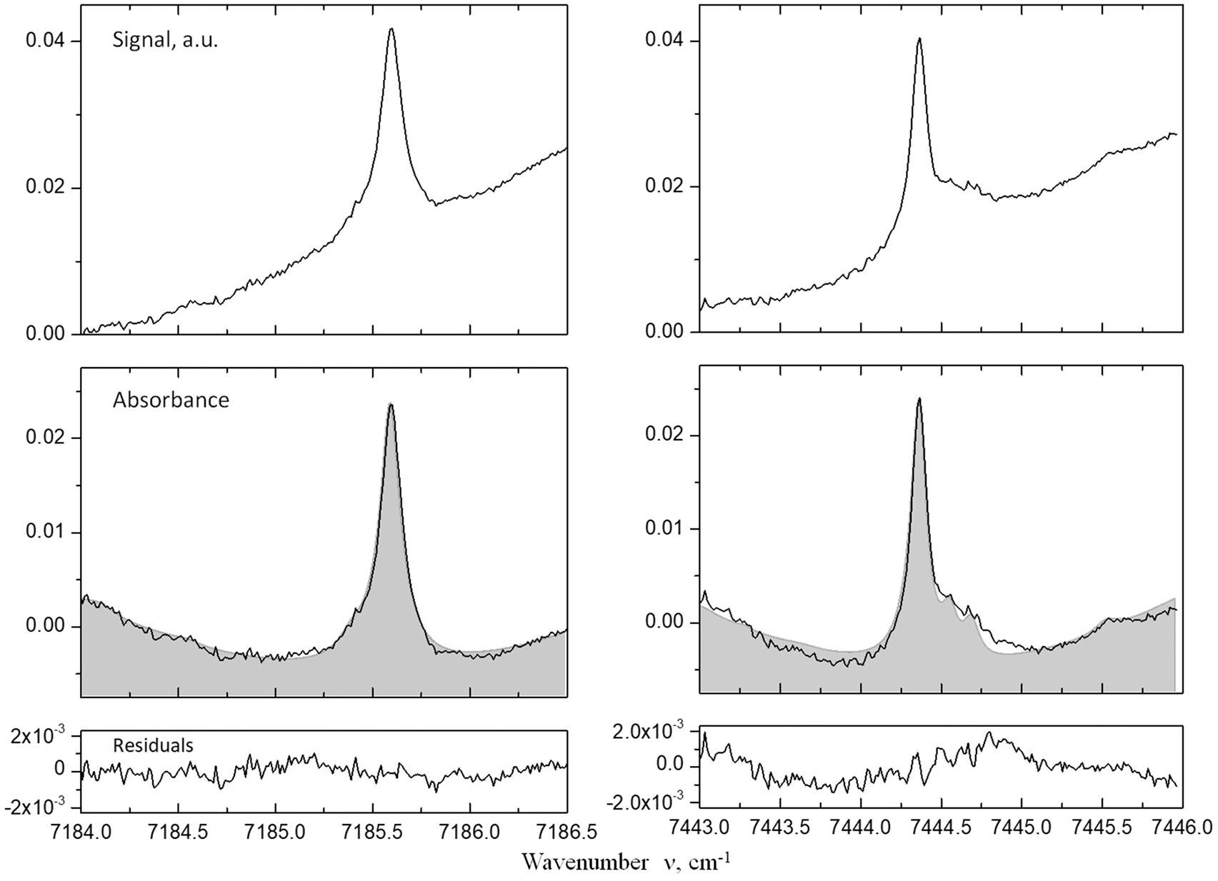

A reasonable question is the number of components to be subtracted from the raw data. In fact, there are no theoretical ab initio criteria for the problem. In all cases, one has to examine the structure of raw spectra and check which polynomial order should be used in the fitting procedure. We have examined the dependence of the temperature evaluation on the number of components of the polynomial expansion used for spectra modification. For the spectra in Fig. 4 the results of these estimations are presented in Fig. 5. A very important point is the unknown actual temperature in the hot probed zone of the propulsion system, which makes it rather problematic to estimate the accuracy of the temperature evaluation. Besides, the subtraction of the only linear component (#1 in Fig. 5) results in a higher temperature, compared to the rest of the trace. The addition of the fourth component (cubic) in spectra modification provides a temperature of 1172 K, which is aproximately the same. The subtraction of two to six components (Fig. 5) provides variations in the temperature evaluation less than 50 K, which seems acceptable for such measurements. Thus, for the spectra presented in Fig. 4, the subtraction of only the first three components is adequate.

Figure 5.

Dependence of the evaluated temperature on the number of subtracted components of polynomial expansion for the experimental data presented in Fig. 4.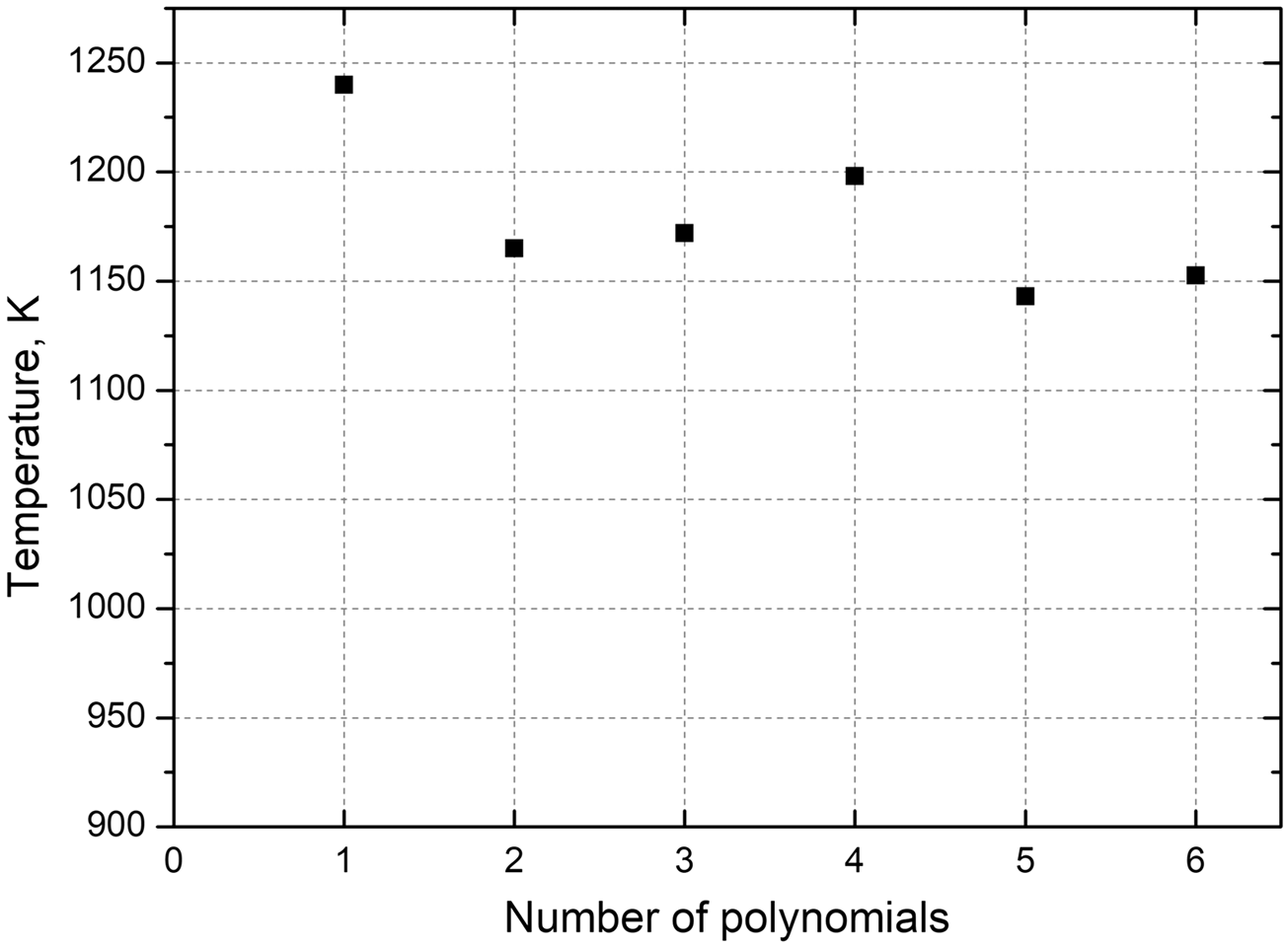

Conclusion

A new algorithm for the evaluation of the integral line intensities of the absorption lines in case of undefined BL and noises is proposed. This situation is crucial, for example, in measurements of the temperature using DLAS. The algorithm is based on the expansion of the experimental and simulated spectra in a series of the orthogonal polynomials, reduction of the first components from the experimental and simulated spectra, and fitting of thus modified spectra. Advantages and disadvantages of the proposed algorithm in comparison with the usually used ones are demonstrated in the numerical experiments. The dependences of the mean $\bar{S}$ and standard deviation sd(S) of the integral intensity evaluation on the linewidth are discussed. Finally, the standard deviation of the temperature evaluation based on the estimated values $\bar{T}$ and sd(T) are obtained.

The proposed algorithm allows avoiding simultaneous fitting of the BL during the general fitting of the experimental and theoretical spectra. Although the final results of the procedures using the “simultaneous” fitting and subtraction of the polynomials are basically similar, the subtraction algorithm minimizes the number of variables in the fitting process. In a traditional simultaneous procedure, the coefficients for the BL are independently varied, while the polynomial projections are calculated using the defined recurrent formulas.

In the numerical experiments, the white noise (2% of the line amplitude) and the BL in the form of parabola were used. For the line HWHM in the range of 0.02–0.6 cm⁻¹, the rsd(S) was in the range of 0.02–0.04, which corresponds to the variation of sd(T) from 30 K to 60 K for the mean temperature of 1000 K.

The proposed algorithm was applied to the fitting of real experimental spectra registered in the experiments on the test propulsion. The H₂O DLAS spectrometer was based on two DLs working in the 7185 cm⁻¹ and 7444 cm⁻¹ ranges. Following the developed algorithm, the raw and theoretical spectra were modified by subtraction of the first three components of the polynomial expansion. The evaluated temperature in one scan of DLs (40 ms) was estimated to 1165 K. Fitting of the experimental spectra with subtraction of the components up to six gives the variation in the estimated temperature within 50 K.

Footnotes

Conflict of Interest

The authors report there are no conflicts of interest.

Funding

The partial financial support from Russian Academy of Sciences via the grant “Basic Problems of Laser Technologies” is acknowledged.

References

Allen

M.G.

“Diode Laser Absorption Sensors for Gas-Dynamic and Combustion Flows”. Meas. Sci. Technol. 1998. 9(4): 545–562.

Hanson

R.K.

“Applications of Quantitative Laser Sensors to Kinetics, Propulsion and Practical Energy Systems”. Proc. Combust. Inst. 2011. 33(1): 1–40.

Bolshov

M.A.

Kuritsyn

Yu.A.

Romanovskii

Yu.V.

“Tunable Diode Laser Spectroscopy as a Technique for Combustion Diagnostics”. Spectrochim. Acta, Part B. 2015. 106: 45–66.

Goldenstein

C.S.

Spearrin

R.M.

Jeffries

J.B.

Hanson

R.K.

“Infrared Laser-Absorption Sensing for Combustion Gases”. Prog. Energy Combust. Sci. 2017. 60: 132–176.

Rothman

L.S.

Gordon

I.E.

Babikov

Barbe

Chris Benner

et al.

“The HITRAN2012 Molecular Spectroscopic Database”. J. Quant. Spectrosc. Radiat. Transf. 2013. 130: 4–50.

Rothman

L.S.

Gordon

I.E.

Barber

R.J.

Dothe

Gamache

R.R.

et al.

“HITEMP, the High-Temperature Molecular Spectroscopic Database”. J. Quant. Spectrosc. Radiat. Transf. 2010. 111(15): 2139–2150.

Werle

“A Review of Recent Advances in Semiconductor Laser Based Gas Monitors”. Spectrochim. Acta, Part A. 1998. 54(2): 197–236.

Zhao

Chen

“A Review of Signal Enhancement and Noise Reduction Techniques for Tunable Diode Laser Absorption Spectroscopy”. Appl. Spectrosc. Rev. 2014. 49(8): 666–691.

Philippe

L.C.

Hanson

R.K.

“Laser Diode Wavelength-Modulation Spectroscopy for Simultaneous Measurement of Temperature, Pressure, and Velocity in Shock-Heated Oxygen Flows.”. Appl. Opt. 1993. 32(30): 6090–6103.

10.

Kranendonk

L.A.

Caswell

A.W.

Sanders

S.T.

“Robust Method for Calculating Temperature, Pressure, and Absorber Mole Fraction from Broadband Spectra”. Appl. Opt. 2007. 46(19): 4117–4124.

11.

Wang

Sanders

S.T.

Jeffries

J.B.

Hanson

R.K.

“Oxygen Measurements at High Pressures with Vertical Cavity Surface-Emitting Lasers”. Appl. Phys. B. 2001. 72(7): 865–872.

12.

Bolshov

M.A.

Kuritsyn

Yu.A.

Liger

V.V.

Mironenko

V.R.

et al.

“Measurements of the Temperature and Water Vapor Concentration in a Hot Zone by Tunable Diode Laser Absorption Spectrometry”. Appl. Phys. B. 2010. 100(2): 397–407.

13.

Bolshov

M.A.

Kuritsyn

Yu.A.

Liger

V.V.

Mironenko

V.R.

“Development of Diode Laser Absorption Spectroscopy Method for Determining Temperature and Concentration of Molecules in Remote Object”. Opt. Spectrosc. 2011. 110(6): 848–856.

14.

Simms

J.M.

Brittelle

M.S.

Ramesh

et al.

“Simultaneous Optimization Method for Absorption Spectroscopy Postprocessing”. Appl. Opt. 2015. 54(14): 4403–4410.

15.

Witzel

Klein

Wagner

Meffert

et al.

“High-Speed Tunable Diode Laser Absorption Spectroscopy for Sampling-Free In-Cylinder Water Vapor Concentration Measurements in an Optical IC Engine”. Appl. Phys. B. 2012. 109(3): 521–532.

16.

Caswell

A.W.

Roy

Sanders

S.T.

et al.

“Measurements of Multiple Gas Parameters in a Pulsed-Detonation Combustor Using Time-Division-Multiplexed Fourier-Domain Mode-Locked Lasers”. Appl. Opt. 2013. 52(12): 2893.

17.

Sanders

S.T.

Wang

Jeffries

J.B.

Hanson

R.K.

“Diode-Laser Absorption Sensor for Line-of-Sight Gas Temperature Distributions”. Appl. Opt. 2001. 40(24): 4404–4415.

18.

Kelley

C.T.

Iterative Methods for Optimization. Philadelphia, PA: Siam, 1999.

19.

Strutz

Data Fitting and Uncertainty. 2nd. Vieweg: Springer, 2016.

20.

“Least-Squares (Model Fitting) Algorothms”. MathWorks. http://www.mathworks.com/help/optim/ug/least-squares-model-fitting-algorithms.html.

21.

Forsythe

G.E.

“Generation and Use of Orthogonal Polynomials for Data-Fitting with a Digital Computer”. J. Soc. Ind. Appl. Math. 1957. 5(2): 74–88.

22.

Hudson

D.J.

Statistics Lectures II: Maximum Likelihood and Least Squares Theory. Geneva: CERN, 1964.

23.

Bolshov

M.A.

Liger

V.V.

Kuritsyn

Yu.A.

Mironenko

V.R.

et al.

“Measurement of the Parameters of the Non-Stationary Gas Flows with High Temperature and Pressure by Diode Laser Absorption Spectroscopy”. Opt. Spectrosc. 2017. 122(5): 20–29.

24.

M.A. Bolshov, V.V. Liger, Yu.A. Kuritsyn, V.R. Mironenko, et al. “Measurement of the Parameters of Non-Stationary Gas Flows by Diode Laser Absorption Spectroscopy in Case of High Temperature and High Pressure”. EPJ Web Conf. 2017. 132: 01001.