
Abstract
The use of rotating filter wheels is common in photometric applications. Traditional filter wheel designs typically exhibit a number of filter openings spaced evenly about the circumference of the wheel. In this work we examine a number of shortcomings of this traditional filter design in measurements of phytoplankton fluorescence made with our fluorescence imaging photometer (FIP). We present an alternative asymmetric wheel design that offers a number of advantages over the traditional design as well as a new processing algorithm designed to accommodate convolution of signals from adjacent channels inherent in measurements collected with the asymmetric design. This approach eliminates the need for a separate signal to establish timing and wheel position, unambiguously establishes filter order even when the direction of rotation is unknown, allows for better estimates of signal baseline, and is more resilient to effects of vibration and other dynamic processes that could occur on the time scale of wheel rotation. We demonstrate performance improvements for phytoplankton fluorescence measurements associated with the new wheel design and algorithm compared with previously published methods using the FIP. Both the improved image processing algorithm and filter wheel design were found to reduce noise in our measurements significantly.
Keywords
Introduction
Optical measurements in photometer systems often employ filter wheels. In past reports, our lab has described the use of a filter wheel on the excitation arm of an asynchronous fluorescence imaging photometer (FIP) for classification of phytoplankton cells.1–4 The asynchronous character of the measurements resulted from the fact that phytoplankton entered the field of view of the instrument at random times, so there was no exact correlation between the appearance of a phytoplankton cell and the position of the filter wheel. Instead, the position of the filter wheel had to be inferred from measurements of the phytoplankton fluorescence recorded on a single charge-coupled device (CCD) camera frame as the cell passed through the field of view of the camera.
The filter wheel used in these earlier studies was of a traditional design with six evenly spaced openings for filters. Results consisted of ratios of measurements made through matched pairs of filters. While satisfactory, there were several aspects of the wheel that we felt could be improved for asynchronous fluorescence imaging.
One drawback of the original filter wheel was that one opening was blocked to provide a reference timing mark in data from each rotation of the wheel. This allowed us to match fluorescence measurements to filters in the remaining five positions as detailed by Pearl et al. 3 Thus, one of the filter wheel positions was sacrificed for timing purposes, and only five data channels were usable, meaning that only two unique matched pairs of filters could be used instead of three. An alternate form of timing could recover the sixth filter channel and enable a third unique pair in the same wheel.
A second drawback with the original filter wheel was due to image blur interfering with observation of the baseline intensity between filter measurements. The same effect occurs in non-imaging filter wheel instruments when the detector response is too slow relative to the filter wheel rotation speed to settle properly between filter openings, or when light leaks through adjacent filters, or if a sample presents delayed fluorescence. The solution for these problems is to increase the spacing or the time delay between adjacent filter wheel openings, or decrease the frequency of rotation of the wheel. Each of these possible solutions involves tradeoffs in signal to noise ratio or sampling frequency.
In the FIP, the proximity of filters in the filter wheel often resulted in image profiles that reached baseline only during the period when the “blank” filter was in the path of excitation light. Because filter wheel rotation frequency and cell flow rates were typically set such that a cell remained within the field of view for only slightly longer than one full rotation of the filter wheel, baseline estimations would typically be carried out with only one “blank” measurement. This produced a single-point baseline measurement that gave no information on baseline slope or curvature. It was not possible to estimate a specific baseline value for each matched pair of filters, for instance, which would have improved precision. Better baseline resolution could be obtained by moving filters further apart on the wheel.
A third issue with the original wheel design was that it was mechanically symmetric: it could be assembled backwards, rotated in the opposite direction, or the filters could be loaded in reverse order, and nothing in the data could reveal the error after the fact. This had the potential to cause issues if different operators were setting up the instrument, and the “standard” orientation, rotation direction and filter ordering of the wheel were not clearly conveyed and understood. Errors in orientation, rotation or filter loading would lead to misidentification of filter pairs and inversion of filter pair ratios, which could result in misidentification of phytoplankton species. This could be avoided or diagnosed and repaired after the fact if the filter wheel were asymmetric.
A final area for improvement resulted from an analysis of covariance between filter measurements. In the presence of vibration or other sources of system variability, the correlation between measurement channels can vary significantly. Measurements made with adjacent filters under these circumstances exhibited greater correlation than measurements taken further apart in time or, equally, system noise is introduced as filter measurements are sampled further apart in time. A significant improvement to measurement signal-to-noise ratio (SNR) could be realized by moving matched filter pairs closer together on the wheel, allowing pairs of measurements to be taken closer together in time without changing the rotation frequency of the wheel.
These four considerations led us to examine the asymmetric filter wheel design depicted in Fig. 1a. In this design, paired filter openings have an angular separation of 30° and the centers of the three filter pairs are separated from one another by angles of 110°, 120°, and 130°. This asymmetric spacing allows us to establish both filter order (eliminating the need for a blank) directly from the fluorescence measurement and gives the filter wheel a handedness to confirm filter wheel orientation as well. The larger gaps provide better opportunity for the signal to reach baseline between pairs so any irregularity of the baseline can be observed. Finally, the smaller gaps within each pair of filters reduces time dependence in measured fluorescence intensities due to vibration, lamp fluctuation, fluorescence efficiency modulation, etc., that might vary on the time scale of wheel rotation.
Simplified schematics of (a) the asymmetric six-position filter wheel and (b) the traditional six-position filter wheel design. Angles between filter pairs in (a) and filters in (b) are indicated in gray.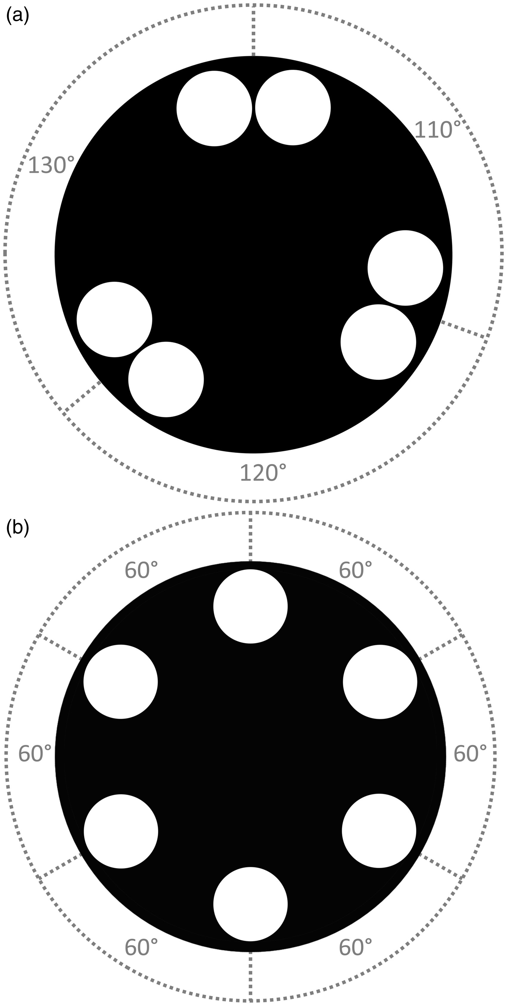
These improvements are obtained at the cost of overlap between the fluorescence emission signals of paired measurement channels, requiring the deconvolution of fluorescence intensity contributions of the two channels in each pair. This manuscript describes the performance of the modified filter wheel for asynchronous fluorescence measurements compared to the original symmetric design, as well as the algorithm used for the deconvolution of filter pair signals.
Experimental
Filter Wheel Design and Fabrication
The asymmetric filter wheel was designed and fabricated in-house. The wheel has a diameter of 5.25 inches (13.335 cm) and filter positions are 1 inch (2.54 cm) in diameter and are centered 2 inches (5.08 cm) from the center of the filter wheel. Asymmetric filter wheel measurements were compared with measurements made using a traditional six-position filter wheel (Part number #56-658, Edmund Optics) of the same size, also with 1-inch (2.54 cm) diameter openings centered on a 2-inch (2.54 cm) radius. Simplified schematics of the two filter wheel designs are depicted in Fig. 1. A detailed description of the FIP setup is presented in Rekully et al.;
5
a simplified schematic of the FIP appears in Fig. 2. Performance comparisons between the two wheel designs were conducted using the same setup described in Rekully et al.,
5
with the traditional filter wheel and asymmetric filter wheel being substituted for one another depending on the condition being tested.
A schematic of the fluorescence imaging photometer (originally shown in Rekully et al.).
5
Excitation light produced by 80 W tungsten halogen lamp (Ex) passes through aperture (K), light pipe (P), and holographic diffuser (H) before being focused through lenses L1 and L2. Focused light is subsequently passed through a 625 nm short-pass filter (F1) before being modulated by one of the six openings in the rotating filter wheel (W). Filtered light is focused through lenses L3 and L4 before striking a beam splitter (BS) and being directed into a 60× microscope objective. Light from the objective is focused in the center of a flow cell (C) through which phytoplankton are being pumped. Cells absorb the excitation light and emit fluorescence, which passes through the microscope objective and the beam splitter and is filtered by a red colored glass filter F2, and a 680 ± 10 nm bandpass filter before being focused by L5 onto a CCD array (D).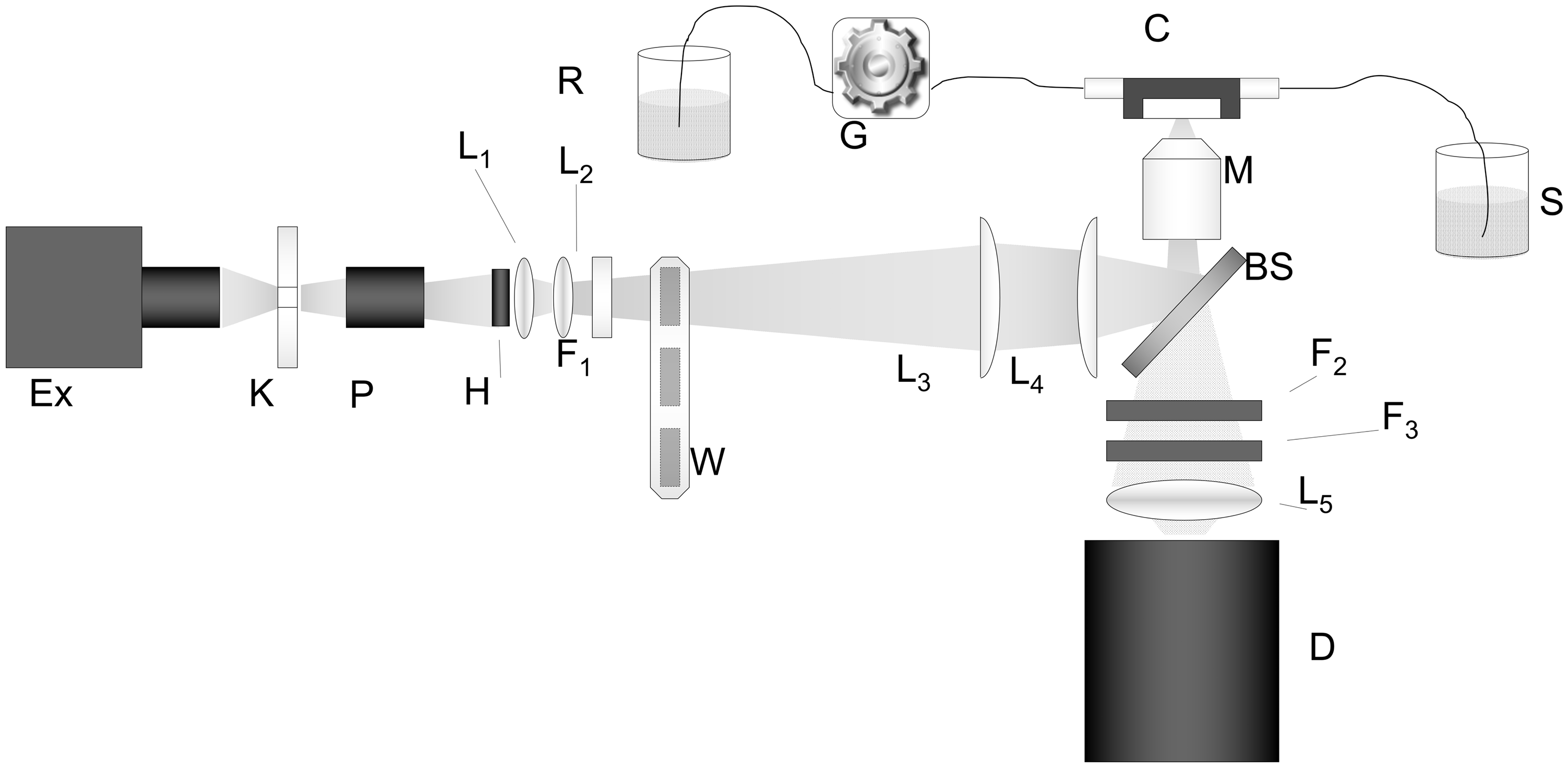
Samples for Performance Comparison
Performance of the filter wheels was compared by measuring the variance of fluorescence ratio signals excited from cells of the diatom Thalassiosira pseudonana using the filter wheels without filters, i.e., open filter positions. T. pseudonana was selected for this demonstration due to the relatively high SNR observed in previous measurement sets. The use of open filter positions rather than one of our previously described filter sets was driven by a desire to eliminate variance in fluorescence ratio uncertainties due to cell-to-cell differences in pigmentation. Except for measurement uncertainty, each filter opening should excite the same fluorescence intensity.
The T. pseudonana strain (CCMP 1335) used in this demonstration was acquired commercially from the National Center for Marine Algae and Microbiota (NCMA, East Boothbay, Maine) and was cultured using the procedure described by Bruckman et al. 4 Sets of 2000 images of each species were collected using each of the two filter wheel conditions along with 100 background images and 100 flat field images collected according to the procedure described by Pearl et al. 3 Image sets collected with the new asymmetric filter wheel design were processed using a new method described below, while images collected with the symmetric filter wheel design were processed using both the automated algorithm, described by Pearl et al., 3 and a modified version of the algorithm described below.
Asymmetric Filter Wheel Image Processing Algorithm
Track Identification
All sample images are first background subtracted and flat-field corrected using the procedure described by Pearl et al.
3
Phytoplankton “tracks” (areas of images that contain phytoplankton fluorescence) are then identified using autocorrelation of each column to determine whether a track is likely to be present, again, using the procedure described by Pearl et al.
3
An autocorrelation threshold is established for each image set by determining the autocorrelation of all columns in a background image set (corrected in the same manner as the sample image set) and setting the threshold as the average plus-two standard deviations of the average background autocorrelation of each column. Adjacent columns that exceed the threshold in each image are grouped together and edges of these groups are identified to give a preliminary estimate of the bounds of potential tracks in the set. Autocorrelation trends within each boundary are then examined. A well-focused track typically has a single autocorrelation maximum near its center; thus, when multiple maxima are found within the bounds of a single track, it is usually an indication that multiple tracks are present. When this situation is observed, the existing track is divided into multiple tracks with local minima between each pair of maxima serving as boundaries between the newly divided tracks. A pseudocolor image containing two track produced by the asymmetric filter wheel with bounds determined by the process described above appears in Fig. 3.
Example of a pseudocolor image of fluorescence intensity produced by two Thalassiosira pseudonana cells traveling through the field of view of the fluorescence imaging photometer as the excitation is modulated by the asymmetric filter wheel. The image contains two fluorescence tracks that passed all quality tests. Solid and dashed red lines represent optimized left and right boundaries for each of the two tracks. Axis labels give the dimensions of the imaged area. Cells move from the bottom to the top of the image over the course of approximately 100 ms, and all images are taken with a CCD shutter speed of 1 s. As a result, while the two tracks appear side-by-side they could have traveled through the frame at any time during a 1 s interval.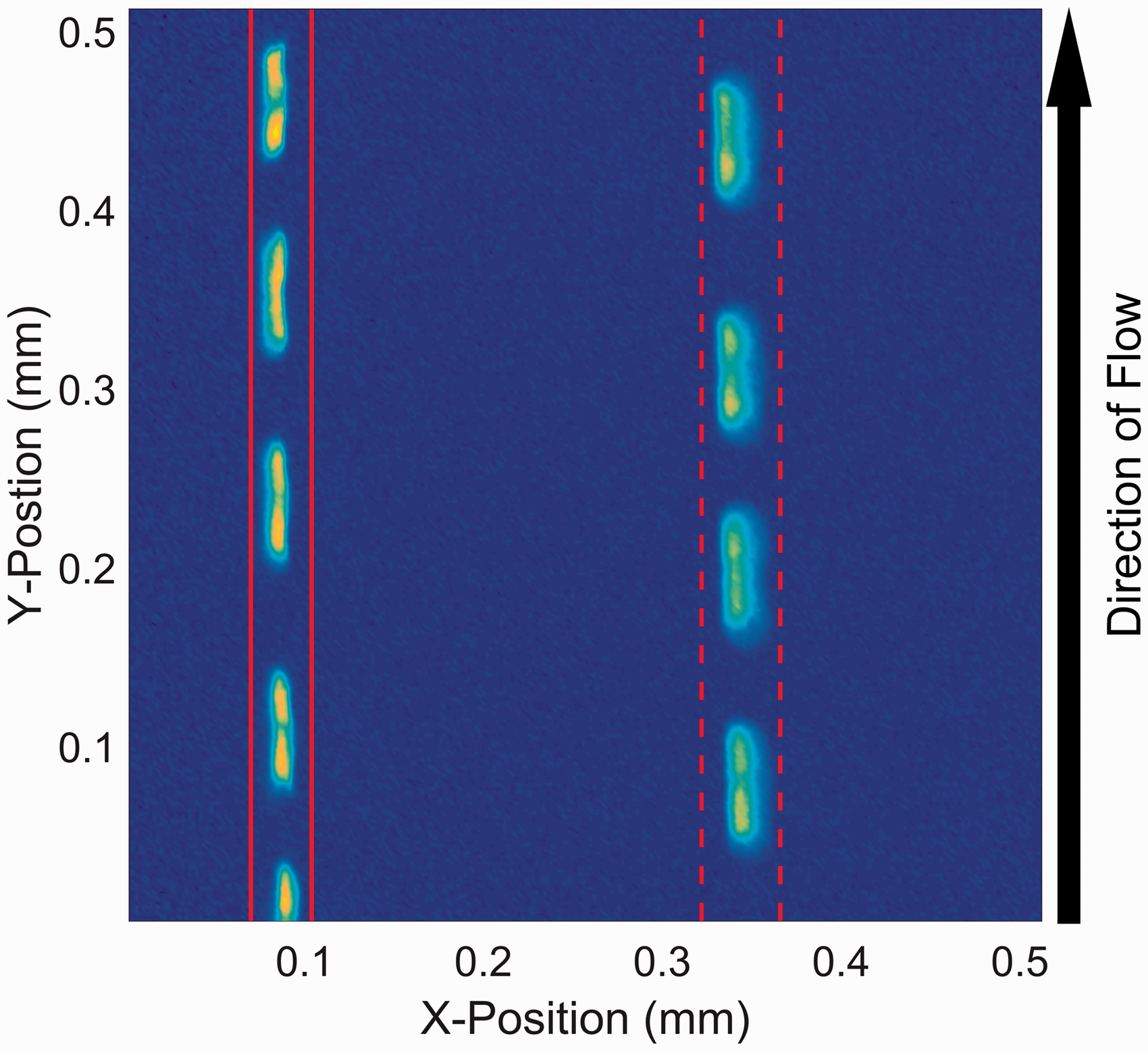
Initial Quality Tests
Once initial track boundaries have been delineated, several tests are applied to each track to determine if the track is of sufficiently high quality to produce useful results during the line shape fitting procedure. These tests are empirically derived. Each of the tests is devised as a means to reject tracks that are beyond the ability of our current algorithms to accurately characterize. In the development of this algorithm, groups of tracks that were identified as outliers were examined to see if they would have been rejected by eye in a manual test. When the answer to that question was in the affirmative, a new test was developed that attempted to quantify the feature that would have led to a manual rejection. The result was tests that were simple and empirical.
Once such a test has been conceived, the threshold for accepting or rejecting a track is optimized through a manual process in which several FIP datasets of different phytoplankton species are subjected to the new test at varying thresholds and a level is found at which a significant portion of the tracks that cannot be characterized fail, while the vast majority of tracks that can be characterized pass.
Figure 4 provides an example track intensity profile with optimized peak fits (discussed below) and Table I provides quality test information for the example track to better illustrate the quality control (QC) process. An integrated track intensity test (quality test #1) first determines whether potential tracks have sufficient fluorescence intensity for analysis; any tracks with a total integrated intensity (i.e., the sum of the intensities registered by all pixels in the two-dimensional area between the left and right boundary of the track) below 25 000 photon counts are rejected due to the difficulty of fitting profiles to low SNR tracks. An edge proximity test (quality test #2) determines whether tracks have a right or left boundary on the edge of the image. If either bound is at the edge of an image, the track is excluded from further analysis due to the likelihood that a significant portion of total track intensity is not captured in the image. A cut-off track test (quality test #3) is used to identify tracks that do not span the entire length of the image. The total integrated intensity of the 25% of pixels at the top of the track is divided by the total integrated intensity of the 25% of pixels at the bottom. If the ratio is less than 0.1 or greater than 10 the track is removed due to the uncertainty of intensity measurements that are partially “cut off” at the beginning or end of each image collection period.
Example row-integrated intensity profile of a Thalassiosira pseudonana track identified from an image set collected on the fluorescence imaging photometer (in solid red) along with optimized lineshape fits. Optimized profile fits to individual streaks are indicated by dashed lines, and the sum of all optimized streak profiles at each row number is indicated by the line of black stars. Results of eight quality tests compared with test limits for the example Thalassiosira pseudonana track shown in Fig. 3.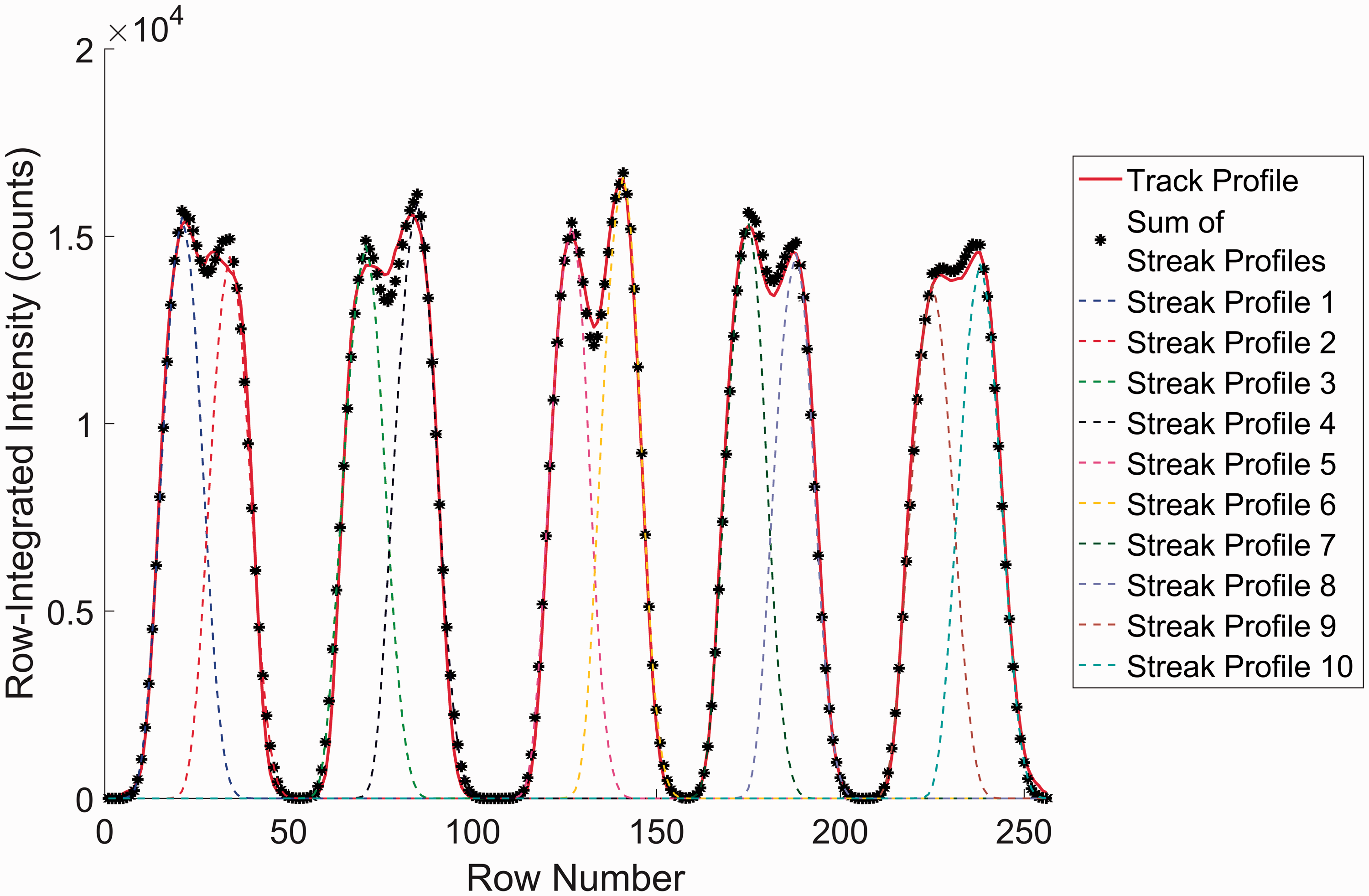
Fitting of Streak Profiles
The primary difficulty inherent in analysis of images produced using the asymmetric filter wheel relative to those produced with the traditional filter wheel design is the overlap of intensity peaks (hereafter referred to as streaks) produced by illumination through filters within each pair. In principle, each overlapped streak pair should be a linear combination of the two component streaks. Based on our knowledge of the intensity profile shapes of non-overlapped streaks collected using wheels with a single open position, we know that streak profiles are not well described by commonly used line shapes such as those produced by Gaussian or Lorentzian functions. In order to find line shape components whose contributions to overlapped streak pair profiles could be optimized in a low-dimensionality search-space, we turned to principal component analysis (PCA) of streak profiles. Performing PCA on a set of isolated streaks (normalized to unit area) from 6000 FIP images each of T. pseudonana, Dunaliella tertiolecta (CCMP 1320), Emiliania huxleyi (CCMP 1516), and Proteomonas sulcata (CCMP 1175) (all species were supplied by NCMA, East Boothbay, Maine) collected using the symmetric filter wheel revealed that ∼99% of the variance in streak profile shape could be described using the first three principal components (PCs). Furthermore, after the elimination of a few outlier scores a cubic relationship was found between scores on PCs 1 and 3, which allowed us to express streak profile shape as a function of two variables.
In addition to the two variables required to specify the shape of a streak (a variable describing scores on PCs 1 and 3 and a variable describing score on PC 2), a magnitude term specifying streak intensity, and another specifying the location of the streak center are required to provide a fitted approximation of a given streak intensity profile. Using this methodology, any streak profile can thus be approximated using a function of four variables. For the simultaneous fitting of overlapped streak pairs, we make the further simplifying assumption that the two streaks within each pair have the same basic shape and differ only in location and magnitude. Thus for the simultaneous fitting of the two streaks within an overlapped pair we can specify a fit using six variables (two for the shape of the streak profiles, two for the center locations of each streak profile, and two for the magnitude of each of the two profiles). Of these, the difference in the two variables describing the peak positions needs to be realistic since it originates in the 30o separation of filters in a pair. With the dimensionality of the problem reduced to a reasonable number of variables we are able to use a nonlinear optimization function to obtain a pair of streak profiles whose sum best approximates the intensity profile of a given overlapped streak pair as determined by a sum-of-squared residuals figure of merit.
Using the procedure described above, each overlapped streak pair of each identified track is fit as a sum of two component streaks, which are then saved for further analysis. An example of optimized streak profile fits to a track profile produced by the asymmetric filter wheel, and the sum of all the individual streak-fit profiles, are shown in Fig. 4.
Tests Applied After Streak Fitting
Several tests are applied after the streak fitting procedure to ensure that fits accurately represent row-integrated streak intensities. A cut-off streak test (quality test #4) seeks to identify streaks that are partially cut-off at the top or bottom of the image. In order to avoid this issue, the intensity of each fitted streak profile is determined at the top and bottom of the image. If the streak profile intensity at the first or last pixel is more than 10% of its maximum value (indicating that a significant portion of the associated fluorescence was not captured in the image) the streak profile is removed from further analysis.
To ensure that at least one full rotation of the filter wheel is clearly observed in the track, the algorithm requires a minimum of four streak pairs (eight total streaks) to be completely contained within the image. Any tracks that contain less than eight streaks are removed from further consideration at this point (quality test #5).
Another issue that can occur is poor resolution of overlapped streak pair profiles from the background. This issue usually arises due to multiple tracks being overlapped, poor boundary selection between two tracks in close proximity to one another, or tracks with so many streaks that the track signal is poorly modulated. A streak resolution test (quality test #6) is used to detect such a scenario. In this test the height of each local minimum between peak pairs in the track profile is compared with the maximum intensity of the adjacent peaks. The track is removed if the smallest ratio is less than two.
A lack of fit test (quality test #7) attempts to assess the overall fit quality to ensure that the track profile is well described by the sum of fitted line shapes. Any tracks with fit intensities that differ from the measured track intensity by more than 20% of the maximum track intensity are considered “poorly fit” and excluded from further analysis.
A final issue that we address after the fitting is difficulty in distinguishing tracks that cross the image at an angle from tracks that are partially overlapped with one another. Due to the relatively large spaces between filter pairs, it is possible for tracks traveling through the field of view at a pronounced angle to produce two or more distinct peak maxima when the track intensity is summed in the y- (the time- or flow-) dimension, this makes them difficult to distinguish from instances in which multiple tracks are partially overlapped or in close proximity to one another. In order to distinguish between these two cases (allowing us to keep angled tracks and exclude overlapped tracks) we instituted a track linearity test (quality test #8) to remove apparent tracks that represent overlapping cell tracks. It first identifies the x,y-positions of streak maxima within a track (y-positions are determined by the fitted streak profiles and x-positions are determined by finding the pixel with maximum intensity in the corresponding row of pixels). Once streak maxima locations have been identified, a linear regression analysis is performed on the resulting set of x,y-points to find a line of best fit. The residuals of streak maxima from the line of best fit are then calculated. If the maximum residual is larger than 10% of the track width, the track fails the test and is removed from further analysis.
Assessment of Cell Speed
The accurate assignment of filter identities (IDs) relies on the ability of the image-processing algorithm to correlate the gaps between pairs of streaks in collected images with the differently sized spaces between adjacent filter pairs on the filter wheel itself. This assignment is complicated somewhat by apparent changes in cell speed during image collection partly caused by spherical aberration in the lens system. In order to obtain a more reliable estimate of the temporal separation of adjacent streak pairs we use the separation between the peak maxima of the two streaks within each pair as a proxy for cell speed. Once this cell speed value has been quantified for each pair of streaks in a track the values can be used with the y-value of the center of each streak pair to fit an interpolated spline allowing us to estimate cell speed at any y-value in the track.
Assignment of Filter IDs
Filter IDs are assigned to streak profiles in the remaining tracks using relative distances between streak centers. The three pairs are separated from one another by spaces of 110°, 120°, and 130°, thus, assuming the wheel spins at a constant rate, the shortest separation between pairs should correspond with the 110° space, the next shortest the 120° space, and the longest the 130° space. Because the cells do not move at a constant pixel/unit time rate we use our speed values described in the preceding section to estimate a temporal separation between peak pairs. By determining the sequence of gap spacing (in terms of relative estimated time) we can use the known placement of filters to assign filter IDs to each streak and determine the direction of rotation.
New Symmetric Filter Wheel Image Processing Algorithm
In order to differentiate between the effects of changing filter wheel designs and changing processing algorithms, a modified version of the asymmetric filter wheel image-processing algorithm was adapted to analyze symmetric filter wheel image data. This algorithm is nearly identical in form and function to the asymmetric processing algorithm described above, aside from a few notable differences. One difference is that, because streaks produced by the symmetric filter wheel have little overlap, each streak is fit independently in the symmetric processing algorithm instead of pairs of streaks being fit simultaneously. The other notable difference is that filter IDs are assigned by identifying the largest separation between streak centers (as the blank filter) and assuming a known direction of rotation to assign IDs to streaks based on their positions relative to the blank.
Results and Discussion
Blocker Versus Asymmetric Spacing Between Streak Pairs for Filter Assignment
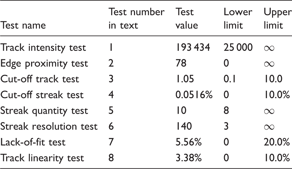
Figure 5a provides an example of a track profile produced using a conventional symmetric filter wheel with a blocker to determine filter sequence in asynchronous measurements, while Fig. 5b provides an example of a track profile produced using the asymmetric filter wheel.
Example row-integrated track intensity profiles for Thalassiosira pseudonana cells collected on the fluorescence imaging photometer using the (a) symmetric and (b) asymmetric filter wheels and processed using the new track characterization methods.
The location of the blocker filter in Fig. 5a is evidenced by the drop in row-integrated intensity between pixel rows 70 and 90 and establishes filter order for a known symmetric filter wheel orientation/direction of rotation, but sacrifices one of the six filter positions to do so. The order of space widths between partially overlapped streak pairs performs the same function for the asymmetric filter wheel track in Fig. 5b. The difference in spacing is most evident to the eye by comparing the wide baseline regions of the tracks, with three distinct spacings. The first space between peaks (beginning around row 50, repeated near row 210) corresponds with the intermediate filter pair separation on the wheel, the second space between peaks (beginning around row 100) corresponds with the largest separation on the wheel, and the third space between peaks (beginning around row 155) corresponds with the smallest separation on the wheel.
Baseline Resolution and Streak Overlap
Figures 5a and 5b also illustrate the difficulty in achieving baseline resolution of peaks in the conventional symmetric filter wheel under common conditions. One clear baseline region is observed in Fig. 5a due to the blocker. A track exhibiting only one blocker position as seen in Fig. 5a is quite common; in the example T. pseudonana set used only 23.7% of tracks contained more than one instance of the blocker. Thus, for the majority of tracks, the intensity minimum provided by a single blocker instance will be the only opportunity to achieve an estimate of the baseline.
The spacing between pairs in the asymmetric wheel is nearly as large as the spacing including the blocker on the symmetric wheel, so baseline regions are observed in Fig. 5b between each pair of filters. This enables any deviation from a flat baseline to be identified and corrected.
Conversely, the signal produced by each individual filter is less overlapped with neighboring signals in Fig. 5a for the symmetric wheel. The signals for filters in Fig. 5b are strongly overlapped because the filter pairs are so close together on the wheel that light can pass simultaneously through both at the same time at points during measurement. While this appears to be a problem, note that many filter streaks in data from the symmetric filter wheel partially overlap those caused by two other filters. Deconvolution of the individual filter signals is complicated by the number of signals that have to be simultaneously deconvoluted. The asymmetric wheel causes stronger overlap, but each doublet is self-contained.
Estimates of Filter Wheel Rotation/Orientation from Track Profiles
A final set of insights that may be gleaned from Fig. 5 relates to use of the asymmetric filter spacing to determine the direction of wheel rotation directly from the track data. As mentioned above, filter IDs were assigned to each streak in the track shown in Fig. 5b by identifying the small, intermediate, and large spaces between streak pairs. While we have detailed the use of this feature for simple filter assignment with a known filter wheel orientation, the system could be designed to automatically recognize a reversal of wheel orientation, direction of rotation, or direction of fluid flow. Any of these three changes would produce track profiles resembling mirror images about the y-axes in Fig. 5. In Fig. 5a such a change would be impossible to detect based on the track profile alone since the sole point of reference is the location of the blocker. An error inverting the track data would lead to misassigned filter IDs and spurious results. Depending on the number and organization of the filters in the wheel, these spurious results might not be obvious without running calibration samples. The perceivably asymmetric spaces between filter pairs shown in Fig. 5b, however, provide a readily available means of determining filter order in all cases of reversal. Instead of the gap size order of medium → long → short → medium, a mirror image of the track profile would have a gap size order of medium → short → long → medium. Thus as long as we know the physical placement of filters within the asymmetric filter wheel for a given dataset, the direction of rotation does not affect our ability to accurately assign filter IDs to streaks in any given track.
Fluorescence Correlation
Previous work from our laboratory indicated a source of dynamic variability in phytoplankton signals whose origin was unclear. 2 This dynamic variability leads to increased “noise” in measurement ratios as the individual signals are measured further apart in time. The final motivation for redesigning the filter wheel was to reduce the time between filter pair measurements without changing the filter wheel speed and signal intensities, with the aim of reducing the apparent noise.
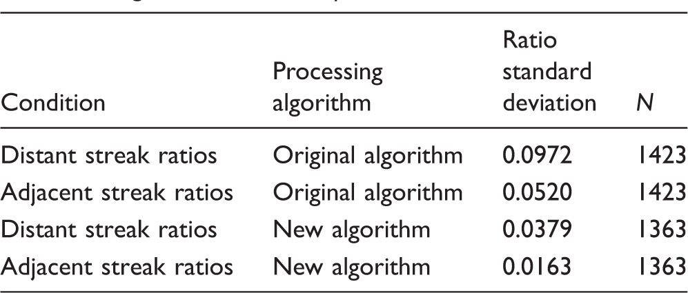
Since single-cell measurements are reported as ratios, we use pairs of open positions to calculate streak intensity ratios using the formula:
Standard deviation and sample sizes for distant and adjacent streak ratio distributions generated using the image processing algorithm, described by Pearl et al., 3 and a novel image processing algorithm on a set of 2000 fluorescence imaging photometer images of Thalassiosira pseudonana.
The original work reported in Swanstrom et al. used only the conventional six-position filter wheel design with a blocker and the older image processing algorithm described there. 2 The asymmetric filter wheel data cannot be processed with that original algorithm because of the need for streak deconvolution, thus the newer algorithm described above was developed. Because the new algorithm improved on the original in several ways, a version of the new algorithm for analyzing symmetric filter wheel data was also created. Both the improved algorithm and the new filter wheel design impact the apparent signal “noise,” so two tests were done in an effort to deconvolute the impacts of these two improvements.
In the first set of tests, the symmetric filter wheel was used to measure signal variability between adjacent and distant filter wheel openings using both the original algorithm and the newer algorithm. The two notable differences between the symmetric and asymmetric wheel versions of the new algorithm (fitting streaks independently due to reduced overlap and using the single available blank on the symmetric filter wheel rather than asymmetric spacing between streak pairs to establish filter order) should have relatively little impact on results obtained. What impact there is should favor the symmetric filter wheel since it does not require disambiguation of paired filter signals.
F-test of equality of variance results for comparisons of original and new image processing algorithms on symmetric filter wheel streak ratios generated with distant and adjacent streaks. F is the ratio of variances and Fcrit is the critical value of the F-statistic at the α = 0.05 level corrected for multiple comparisons using the Bonferroni correction. 6
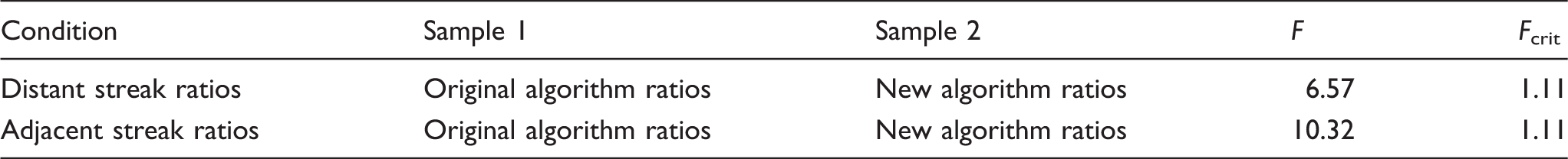
Table II also establishes that the new algorithm, while improving on the original, does not eliminate the increase in apparent “noise” with increasing time between signal measurements in the fluorescence ratio. The standard deviation of ratios generated using adjacent streaks is 0.0163, which is about 56% lower than the standard deviation of ratios generated using distant streaks. We can show the significance of this difference in variance using an F-test of equality of variances with an α = 0.05 critical value. We find an F value of 5.41, which exceeds the critical value of 1.09 for the given α and degrees of freedom specified from population sizes in Table II. Thus we may proceed with reasonable confidence in our assertion that measurements taken closer together in time exhibit a greater degree of correlation.
Again, this points to a time-dependent random process affecting the signal. Dynamics of this type could result from a moving heterogeneous sample; photochemical decay; Brownian rotation and diffusion of cells in suspension; mechanical vibration of the apparatus; voltage fluctuations in a light source; filter wheel speed fluctuations, etc. Regardless of the source, if the fluctuations occur on the time scale of wheel revolution then measurements closer together in time should improve the precision of measurement, which is the subject of the next set of tests.
The second set of tests compares the variability of adjacent symmetric wheel filter signals and asymmetric wheel paired filter signals to see if the reduced time between measurements in the asymmetric wheel pairs leads to any improvement in apparent signal noise.
Standard deviation and sample sizes for adjacent streak ratio distributions generated using the new image processing algorithms on sets of 2000 fluorescence imaging photometer images of Thalassiosira pseudonana collected using the symmetric and asymmetric filter wheels.
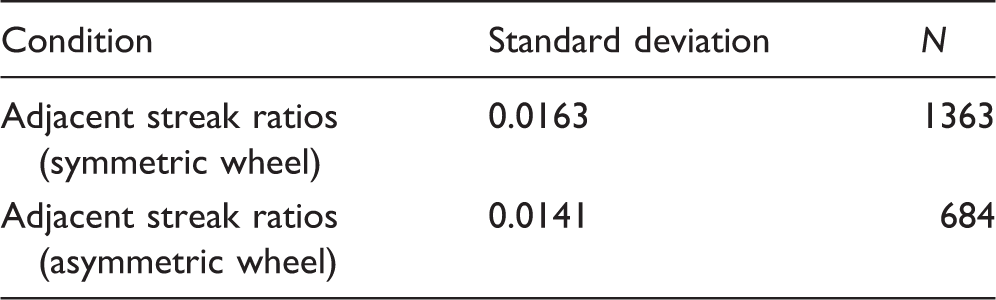
These results show that the change in filter wheel design led to a decrease in ratio standard deviation of about 14% (from 0.0163 to 0.0141). As before we can use an F-test of equality of variances to show whether the statistics presented in Table IV suggest the two wheels produce ratio distributions with significantly different deviations. Testing again at the α = 0.05 level, we find an F-value of 1.31, which exceeds the critical value of 1.12, indicating that the improvement is significant. Because the image processing algorithms used to generate ratios from the two image sets are nearly identical (as described above) we may reasonably conclude that while the bulk of the decrease in ratio standard deviation was realized due to a change in the processing algorithm, the change in filter wheel design is also a statistically significant contributor to standard deviation reduction.
A comparison of the ratio standard deviations in Tables II and IV shows a consistent trend of decreasing standard deviation with decreasing separation in time between measurements. In Table IV, the separation in time between filters in a pair is one-twelfth of a wheel revolution, corresponding to ∼5.4 ms. For the symmetric wheel, adjacent streaks in Table II are separated by one-sixth of a wheel revolution, while distant streaks are separated by about a full wheel revolution. A plot of the ratio standard deviation versus time between measurements (Fig. 6) appears linear with an intercept of ∼0.0120 that corresponds to completely separate measurements made simultaneously on the same cell.
Estimated time gap between streak measurements in milliseconds vs. streak intensity ratio standard deviation for Thalassiosira pseudonana tracks collected using the symmetric and asymmetric filter wheels and processed using the new algorithm. The dashed black line represents a linear fit to the data of the form y = 4.00 × 10⁻⁴(x) + 1.20 × 10⁻².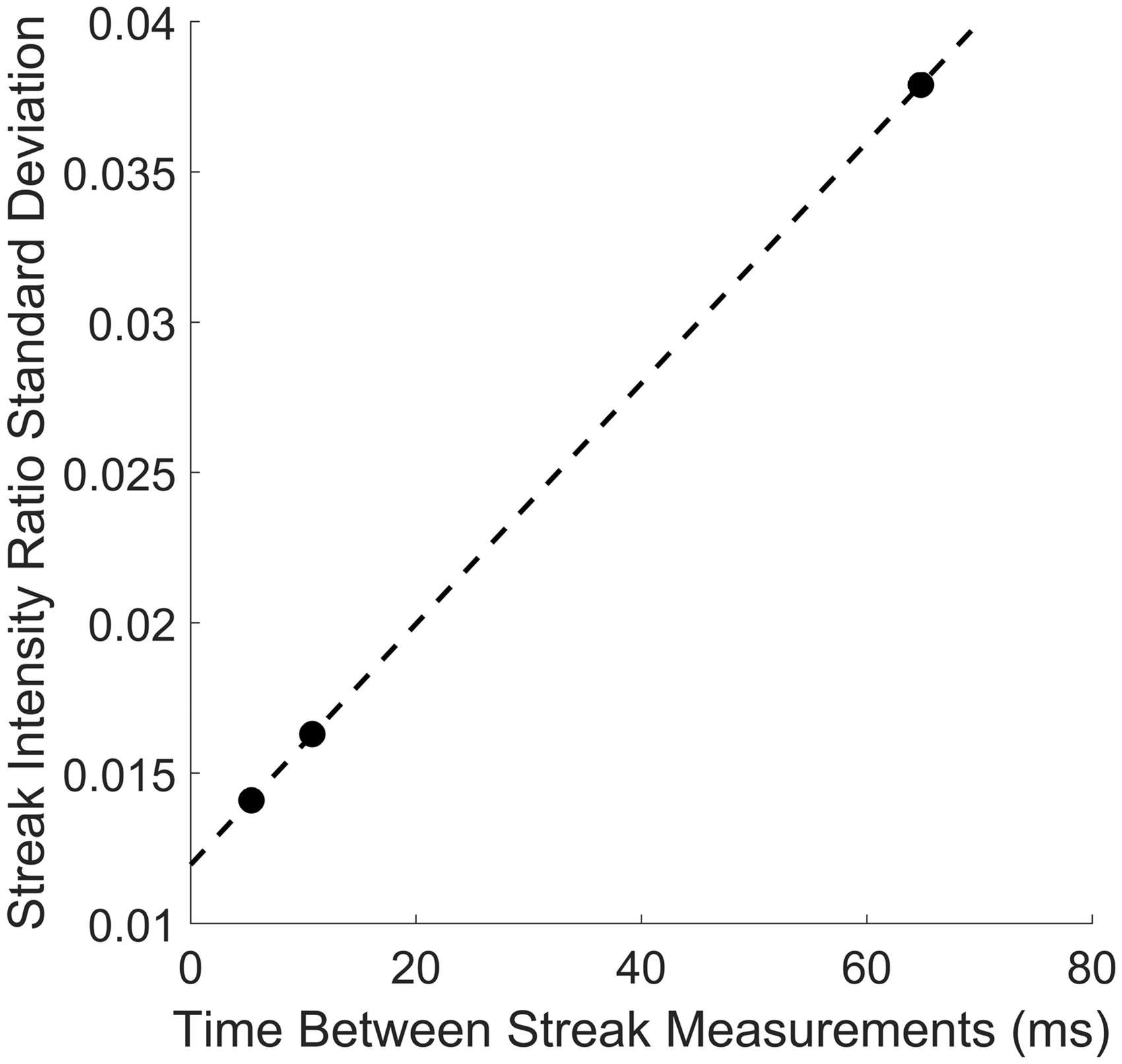
Differences Between Numbers of Tracks Characterized in Each Treatment
In addition to the differences in ratio standard deviation, Table II shows that a small (∼4%) reduction in total number of tracks was observed when the new algorithm is applied to the same data set as the old. This difference can likely be attributed to the quality tests in the new algorithm being somewhat more stringent than the old algorithm. Tests of track linearity and streak intensity reproducibility for instance have no analogue in the original algorithm. When considered alongside the sharp decrease in ratio standard deviation for the new algorithm, it seems reasonable that the bulk of this decrease in number of characterized tracks is the elimination of partially overlapped or poorly delineated tracks (against both of which the earlier algorithm had little defense).
The drop in number of characterized tracks is more dramatic when the asymmetric filter wheel results are compared with the symmetric filter wheel results. The number of characterized tracks is ∼50% lower with the asymmetric wheel than the symmetric wheel results characterized with the new algorithm (see Tables II and IV).
The most important factor explaining the detection of fewer successfully analyzed tracks for the asymmetric wheel data is that a greater number of total streaks are required to be present in an asymmetric wheel track than a symmetric wheel track in order to complete the analysis. While analysis of the symmetric filter wheel requires just six streaks to be contained within the image (ensuring that all filters are represented and at least one instance of the blocker is bracketed by two complete streaks), the asymmetric filter wheel requires that eight complete streaks be contained within the image (ensuring that all three different gap sizes be present for comparison and that a cell speed estimate be made at each point between peak pairs). The majority of tracks collected with the symmetric filter wheel (70.1%) contain only six streaks, 26.9% contain seven streaks, and the remaining ∼3% contain eight or more streaks. If we assume (for simplicity) that the filter wheel is at a mid-point between openings when a cell enters the image and is at another mid-point between openings when the cell leaves the image, the symmetric wheel would need to rotate 420° for a six-streak image and 480° for a seven-streak image. Using the same assumptions, the asymmetric filter wheel would need to rotate between 475° and 485° (depending on the size of the first gap) while the cell crosses the image to achieve the required eight streaks. Both sets of measurements were made with the same pump speed, so we might expect a large percentage of asymmetric wheel data to fail the test for number of streaks under these conditions, and that is what is observed. This type of failure does not bias the data toward higher or lower signals, so it is not expected to affect the noise analysis.
Conclusion
In previous work, 5 we focused on how to design or select filters with greater discriminating power for identifying phytoplankton species with the FIP. In that reference, we concluded, as had others before us,7,8 that binary filters offer the best discrimination in classification measurements. We reported on a new approach to selecting the binary filters for problems involving large and unknown numbers of potential classes, such as the number of distinguishable species of phytoplankton in the world’s lakes and oceans. Along with the realization that there were relatively few factors that distinguish fluorescence excitation spectra of species comes the realization that performance of a single-cell classification system will ultimately be limited by the same factors that limit most measurements, measurement precision. The drive to improve signal extraction, reduce noise, improve standards, etc. has given rise in our laboratory to improvements reported here in the areas of algorithms and signal deconvolution. Other work is aimed at improving the standardization and resampling of phytoplankton in terms of nutrient and light status. By reducing the uncertainty for measurements of phytoplankton, we hope to boost the utility of single-cell phytoplankton analysis at both identifying pigments, species and classes, as well as to use the phytoplankton as indicators of community health and nutrient state (within limits).
The new timing technique available to us through the use of the asymmetric filter wheel not only obviates the need for a blank allowing us to increase the number of unique feature sets used for phytoplankton discrimination, but also allows us to more accurately estimate signal intensities by having more opportunities to sample the baseline. We also have demonstrated that the asymmetric spacing allows us to unambiguously assign filter order even when the direction of rotation is not known. Through a mixture of improved track characterization and QC we have shown that the new image processing algorithm affords much more consistent streak intensity ratios. Finally, we have also demonstrated that significant decreases to streak intensity ratio standard deviation can be realized by collecting paired streak intensities closer together in time. This is a somewhat counterintuitive result since the paired streak intensities wind up strongly overlapped with one another. However, this overlap of pair intensities is counterbalanced by the fact that the overlapped signals have the same underlying peak shape and a consistent separation. The symmetric filter wheel signals also showed a small degree of overlap, but in that case the overlaps were with signals both before and after each filter, with no clear baseline much of the time. In the end, the benefits of decreasing the number of weakly overlapping signals and giving a clear baseline cancelled the drawbacks of needing to deconvolute two strongly overlapped signals.
Footnotes
Acknowledgments
Eric M. Lachenmyer is gratefully acknowledged for maintaining and providing all phytoplankton cultures used in this study. We also thank Art Illingworth and Allen Frye of the Mechanical Prototype Facility for construction of the new filter wheel, flow cells, and other mechanical elements of our instrumentation.
Conflict of Interest
The authors report that there are no conflicts of interest.
Funding
This work was supported by the National Science Foundation’s Division of Ocean Technology and Interdisciplinary Coordination (grant number OCE 0958831).