Long-Term Strategy for Assessing Carbonaceous Particulate Matter Concentrations from Multiple Fourier Transform Infrared (FT-IR) Instruments: Influence of Spectral Dissimilarities on Multivariate Calibration Performance

Abstract

Matching the spectral response between multiple spectrometers is a mandatory procedure when developing robust calibrations whose prediction is independent of instrument-related signal variations. A viable alternative to complex calibration transfer methods consists of matching the instrument spectral response by controlling a set of key instrumental and environmental parameters. This paper discusses the applicability of such an approach to three Fourier transform infrared (FT-IR) spectrometers used for the routine assessment of carbonaceous particulate matter concentrations in the Interagency Monitoring of PROtected Visual Environments (IMPROVE) speciation network. The effectiveness of the proposed matching procedure is evaluated by comparing the spectral response for each individual instrument in order to characterize the extent, and nature, of the remaining inter-instrument spectral dissimilarities. Instrument-related contributions to the signal were determined to be small compared with the spectral variability induced by the filter type used for sample collection. The impact of spectral differences on prediction was addressed through the comparison of model performance derived from multiple calibration scenarios. A hybrid model yielding accurate and homogeneous prediction regardless of the instrument was proposed for organic carbon (OC) and elemental carbon (EC), two major constituents of atmospheric particulate matter. Coefficients of determination of 0.98 (OC) and 0.90 (EC) with median biases not exceeding 0.20 µg (OC) and 0.07 µg (EC) are reported. The long-term stability, assessed from weekly measurements of reference samples, shows a deviation in predicted concentrations of less than ±5% over a 2.5-year period for most of the data collected. Extending OC and EC hybrid models to the prediction of ambient samples collected during the two subsequent years provides satisfactory performance. The proposed instrument matching procedure coupled with the relative simplicity of the hybrid model is an alternative to computationally advanced calibration transfer methodologies for the characterization of carbonaceous particulate matter using multiple FT-IR instruments.

Keywords

Fourier transform infrared spectroscopy FT-IR spectroscopy high sample throughput instrument matching partial least squares PLS hybrid calibration

Introduction

Fourier transform infrared (FT-IR) spectroscopy, which captures structural information associated with molecular composition in a short amount of time, is an attractive analytical technique for the routine monitoring of process controlled operations in food,^1,2 fuel,³ and pharmaceutical industries.⁴ Besides speed, FT-IR is nondestructive, requires little sample preparation, does not involve hazardous solvents, and is relatively robust, making it applicable to indoor and outdoor applications.^5,6 Due to its numerous benefits, including a high sensitivity to organic functional groups, FT-IR spectroscopy has garnered interest in recent years for the characterization of carbonaceous and inorganic particulate matter (PM) deposited on polytetrafluoroethylene (PTFE) filters.⁷ A detailed description of the spectral fingerprint of functional groups commonly encountered in PM and absorbing at specific wavenumbers throughout the mid-IR range is given in the Supplemental Material (Section 1). Due to the complex nature of PM, quantifying function groups such as carbonyl (1650–1800 cm⁻¹) or the aliphatic C–H (≈2900 cm⁻¹) is usually challenging due to the presence of spectral interferences caused by either inorganic compounds or filter-induced light scattering. To address this issue, multivariate regression techniques, such as partial least squares (PLS),⁸ are often employed to develop quantitative models able to predict specific properties of ambient samples including organic carbon (OC),⁹ elemental carbon (EC),¹⁰ major inorganic ions,¹¹ organic functional groups and organic matter (OM).^12,13

Assessing the composition of speciated fine PM emitted or formed in the atmosphere is crucial for understanding its substantial impact on human health,^14,15 climate change,¹⁶ and visibility degradation.^17,18 As PM is known to contain organic compounds, black carbon, soil, sea salt, trace metals, and inorganic ions whose proportion varies temporally and spatially,^19–21 identifying pollution sources and observing local and regional trends in concentrations can best be addressed with consistent measurements across a large region.^22,23 In the United States, routine sampling of atmospheric particles is performed at rural and pristine locations by the Interagency Monitoring of PROtected Visual Environments (IMPROVE, http://vista.cira.colostate.edu/Improve) network while urban and suburban locations are monitored by the Chemical Speciation Network (CSN).^24,25 The CSN comprises about 140 urban sites mostly impacted by anthropogenic emissions related to combustion (fossil fuel burning) and industry while IMPROVE monitors regional impacts and visibility at about 160 rural sites (Supplemental Material, Section 2). Ambient PM samples are collected at every IMPROVE site once every third day and at CSN sites every third or every sixth day generating about 1500 and 1300 samples monthly for IMPROVE and CSN, respectively.

For the sake of maintaining high sample throughput applications, operating multiples spectrometers either in one or several locations is often a prerequisite.^26–28 The main challenge in the development of such measurement platforms lies in the control of the extent of dissimilarities between the response associated with each spectrometer. In practice, any combination of intrinsic factors such as differences in light source aging, optical path, detector response, temperature, or humidity may cause spectral deviations even between nearly identical instruments.²⁹ From a multivariate calibration standpoint, this implies that a calibration model developed on a specific instrument can rarely be extended to the spectra collected on a different instrument or under different experimental conditions without introducing erroneous or biased predictions.³⁰ A straightforward, but time-intensive, approach is to calibrate each spectrometer individually using the same set of standard samples. Conventionally, the need for independent calibration per instrument is often circumvented by either correcting or minimizing instrument-dependent signal contributions so that differences in spectral response between instruments have a negligible impact on model predictions. This way, a specific calibration developed on a target (primary) spectrometer can be universally applied to a network of satellite (secondary) instruments. For this purpose, good practices in spectroscopy involve either spectral preprocessing or advanced standardization procedures.³¹ The latter, also known as calibration transfer, are a series of mathematical algorithms intended to match the response between two instruments by either manipulating their raw spectra or their predicted values.^32–35

The aim of this work is to address the challenges associated with the development of a single instrument-agnostic calibration model for three FT-IR spectrometers used for the routine analysis of IMPROVE and CSN ambient samples. The need for calibration transfer is negated by a careful control of key instrumental parameters and environmental conditions.³⁶ The effectiveness of the instrument matching procedure is investigated by comparing the spectral response of each spectrometer to identify the remaining sources of dissimilarities. The impact of spectral dissimilarities on OC and EC is evaluated through the development of a hybrid model based on IMPROVE samples collected in 2015. The long-term stability of the implemented multivariate calibration model is tested using reference and ambient samples collected in 2016 and 2017 in an attempt to identify instrument drift and foresee situations where instrument recalibration become necessary.

Materials and Methods

Fourier Transform Infrared Spectroscopy

Three FT-IR spectrometers, a Tensor 27 (FTIR1) and two Tensor II (FTIR2, FTIR3) instruments (Bruker Optics), are considered in this work. Each system is equipped with a pre-aligned mid-IR source and a liquid nitrogen-cooled, wideband mercury–cadmium–telluride (MCT) detector with the same nominal specifications. Spectra are acquired in transmission mode over the range 4000–420 cm⁻¹ with a 6 mm source aperture and a resolution of 4 cm⁻¹, yielding 11 138 (zero-filled) data points. A total of 512 scans per sample are collected and averaged to improve the signal-to-noise ratio. The resulting signal is converted into an absorption spectrum using the most recent empty chamber spectrum, acquired hourly.

All three FT-IR spectrometers are located in the same laboratory and were installed in 2011 (FTIR1), 2014 (FTIR2), and 2017 (FTIR3). In May 2016, the two oldest instruments were transferred to a new laboratory situated in the same building, which now houses all three instruments. Mid-infrared spectra of ambient PM samples are collected simultaneously on all three instruments following a random assignment procedure.

Instrument Matching

In an effort to minimize the dissimilarities in spectral response between the three spectrometers, an instrument matching procedure was implemented. The procedure includes a careful control of key environmental and instrumental parameters including sample position, gas phase interferences, detector temperature, and acquisition parameters. Fourier transform IR systems are located less than a few meters apart in a dedicated room to ensure that temperature and humidity variations are consistent across instruments. To prevent external factors from affecting the instruments output, every FT-IR spectrometer is equipped with the systems detailed hereafter. The temperature of the detector is kept below –165 ℃ using an embedded Dewar that is re-filled automatically every 8 h by a liquid nitrogen micro dosing system (NORHOF, The Netherlands). Signal contributions associated with atmospheric water vapor and carbon dioxide are minimized by continuously purging the instruments with a volume control damper (VCD) series CO₂ adsorber/dryer system (PureGas LLC). For an optimal repeatability in sample position relative to the IR beam, a 4.0 × 5.1 × 4.5 cm house-built chamber was specifically designed. Mounted directly inside the default instruments sample compartment, this chamber is connected to the VCD series system to enhance purge efficiency and reduce waiting time before acquisition. A full description of the house-built chamber design and characteristics is available in Sections 3 and 4 in the Supplemental Material, respectively. The total measurement procedure per sample includes a 4 min purge period to minimize atmospheric water vapor and carbon dioxide content in the sample compartment followed by a nearly 1 min spectrum acquisition.

In addition to using instruments from the same manufacturer, with the same hardware and under the same controlled environmental conditions, a careful matching of acquisition settings was also established to reduce the impact of instrument-related intrinsic factors on the spectral response. The matching was achieved by first exporting all acquisition parameters defined on FTIR1 using the OPUS software (Bruker Optics). The subsequent file is then loaded onto the two other FT-IR systems by an automatic procedure before each measurement session. This way, neither the length nor the alignment of the wavenumber channels is compromised across instruments thus preventing the need for spectra interpolation.

Data Sets

In order to address the performance of each spectrometer at different time scales and compare their spectral response, a series of ambient samples, polystyrene standard, field blanks, and reference samples is considered. Ambient samples are routinely collected in the IMPROVE monitoring network by pulling a nominal air volume of 32.8 m³ (24 h sampling time) through a 25 mm polytetrafluoroethylene (PTFE) filter. Samples are collected at nearly 160 pristine sites across the U.S. every third day. Unlike ambient samples, field blanks do not contain PM deposition as the filters are passively exposed during sample collection but no air is pulled through the sample. Finally, reference samples are a fixed set of ambient and blank samples that are analyzed weekly for quality control. For the sake of covering different aspects of the inter-instrument comparison, all available samples are structured into three specific data sets.

The first data set uses spectra from a polystyrene standard and multiple blank filters to identify potential differences in spectral responses between instruments. Polystyrene spectra are acquired daily, once 50 filters have been analyzed, to capture variability in spectral intensity and identify trends over time. A total of 96 (FTIR1), 77 (FTIR2), and 82 (FTIR3) standard polystyrene spectra obtained from February through August 2017 are considered. Additionally, 107 (FTIR1), 113 (FTIR2), and 99 (FTIR3) field blank PTFE spectra measured over the same time period are used to assess the distribution in PTFE signal. To provide further inter-instrument comparison, an ambient PM sample featuring nearly median OC (25.1 µg) and EC (4.2 µg) concentrations is introduced. The latter, sampled on 7 March 2017 at the Wichita Mountains (Oklahoma) IMPROVE site, was analyzed on all three spectrometers.

The second data set is introduced to evaluate the impact of the response of each spectrometer on OC and EC predictions. This set contains spectra from ambient samples analyzed on FTIR1 and FTIR2 as well as duplicate ambient spectra measured on the same instrument. First, a total of 743 ambient samples analyzed on FTIR1 and FTIR2 over a one-year period (2015) were employed to develop and validate a multivariate regression model for OC and EC prediction. Second, duplicate spectra from 265 (FTIR1) and 228 (FTIR2) ambient samples from the same year are used to evaluate instrument precision. Duplicate spectra are acquired within a 1 h time period, once or twice per day per instrument, to assess measurement repeatability. As the number of samples collected on FTIR3 is not yet statistically relevant, the above study is restricted to the two older instruments.

The third data set, designed to monitor the long-term stability of the three spectrometers, is based on a series of four references samples measured weekly as part of a quality control procedure. The former includes two ambient samples collected in Davis, California, USA in 2009, whose composition is stable over time, and two reference blank filters. This study focuses on 1327 spectra of the reference samples measured between February 2015 and September 2017 (FTIR1–FTIR2) and from February 2017 to September 2017 (FTIR3) to identify potential drift in instrument response over time. The ability to predict ambient samples collected in a different year is evaluated by introducing two additional sets of 855 and 391 ambient samples measured in the year 2016 and 2017, respectively. Spectra from 2016 were collected on both FTIR1 and FTIR2 while 2017 spectra were acquired on all three instruments.

Data Analysis

The impact of the instrumental response on OC and EC predictions was addressed by developing a set of multivariate calibration models from the 743 ambient samples measured on both FTIR1 and FTIR2. Since this data set does not include blank filters, model predictions at low concentrations are not satisfactory. For this purpose, a homogeneously distributed set of 50 samples from the blanks data set, selected with the Kennard–Stone algorithm,³⁷ was included in the model to improve the minimum detection limit (MDL). Data partitioning into calibration and test sets was achieved following a base case scenario in which ambient and blanks filters are chronologically stratified by site.⁹ Two-thirds of the ambient spectra along with a series of 34 blank spectra were used to build the multivariate model, yielding a total of 530 calibration samples. The remaining third of the ambient spectra were merged with 16 blank spectra to form a 263 samples test set employed to evaluate model performance. Before developing the model, spectra were centered by subtracting the mean absorbance value at each wavenumber. Fourier transform IR spectra were calibrated against mean-centered OC and EC concentrations provided by the thermal-optical reflectance (TOR) analysis of collocated quartz filters in agreement with the IMPROVE_A protocol (http://views.cira.colostate.edu/fed).³⁸

Although zero-filled spectra (11 138 wavenumbers) are used for visual interpretation, interpolated data points are removed so that only the original data points are used in model development. The processed data yields 2725 channels per spectrum sampled every 1.286 cm⁻¹. Multivariate models were developed using partial least squares (PLS) regression.⁸ Selection of the optimal number of factors, yielding a model with the least prediction error, is achieved via a K-fold cross-validation procedure using K = 5.³⁹ This procedure is repeated for a series of models computed by varying the number of factors. For each model, the root mean square error of cross-validation (RMSECV) is calculated and the number of factors minimizing the RMSECV is selected as optimum.

Data handling and analysis were performed in Matlab R2015a (The MathWorks, Inc.) using the statistics and signal processing toolboxes. Partial least squares calculations were run using the libPLS Matlab package (v.1.9, Changsha Nice City, China).⁴⁰

Figures of Merit

To compare the performance of the models developed in this work, several figures of merit are derived based on the linear regression of the predicted (FT-IR) to measured (TOR) concentrations of test samples. Calculated metrics include the coefficient of determination (R²), the root mean square error of prediction (RMSEP), the bias, the error, and the normalized error. The bias is calculated as the difference between predicted (FT-IR) and measured (TOR) concentrations while the error is defined as the absolute bias. The normalized error for a single prediction is the error divided by the corresponding TOR value. In this work, median bias, error, and relative error values are reported. Two additional TOR independent figures of merit addressing the minimum detection limit (MDL) and the instrument precision are also introduced. MDL is computed as three times the standard deviation of field blank samples while instrument precision is estimated from duplicate spectra following Eq. 1:

Precision = \sqrt{\frac{1}{N} \sum_{i = 1}^{N} \frac{{({\hat{y}}_{i 1} - {\hat{y}}_{i 2})}^{2}}{2}}

(1)

where

{\hat{y}}_{i 1}

and

{\hat{y}}_{i 2}

represents the predicted concentrations of the ith spectra pair and N is the total number of spectra measured in duplicate.

Results and Discussion

Assessment of Spectral Dissimilarities Between Spectrometers

The presence of spectral dissimilarities across instruments is first assessed by evaluating the distribution of absorbance values in a polystyrene standard. Mean absorbance and standard deviation, derived from the peak at 2849 cm⁻¹, are compared in Fig. 1 for each spectrometer. While nearly identical distributions are observed between FTIR1 (0.743 ± 0.005 a.u) and FTIR2 (0.744 ± 0.006 a.u), slightly different values are reported for FTIR3 (0.752 ± 0.003 a.u). Significance testing of absorbance means (t-test) and variances (F-test) at the 95% significance level confirms that the two older instruments show similar accuracy and precision for the measurement of polystyrene absorbance values at 2849 cm⁻¹. However, both older instruments show statistically significant differences with FTIR3 which suggests that (minor) discrepancies may exist even though all three spectrometers share the same instrumentation, environmental conditions, and experimental settings.

Figure 1.

Comparison of accuracy and precision across instruments achieved for polystyrene standard and blank PTFE filters absorbances monitored at 2849 cm⁻¹ and 1210 cm⁻¹, respectively. Dark lines correspond to the mean spectrum per data set and per instrument while peak locations considered to compute distribution parameters are indicated by arrows. The highly absorbing polystyrene peak at 2925 cm⁻¹ is associated with a nonlinear response of the MCT detector. Variability in blank PTFE signal is not representative of instrument precision but of the variability in PTFE material.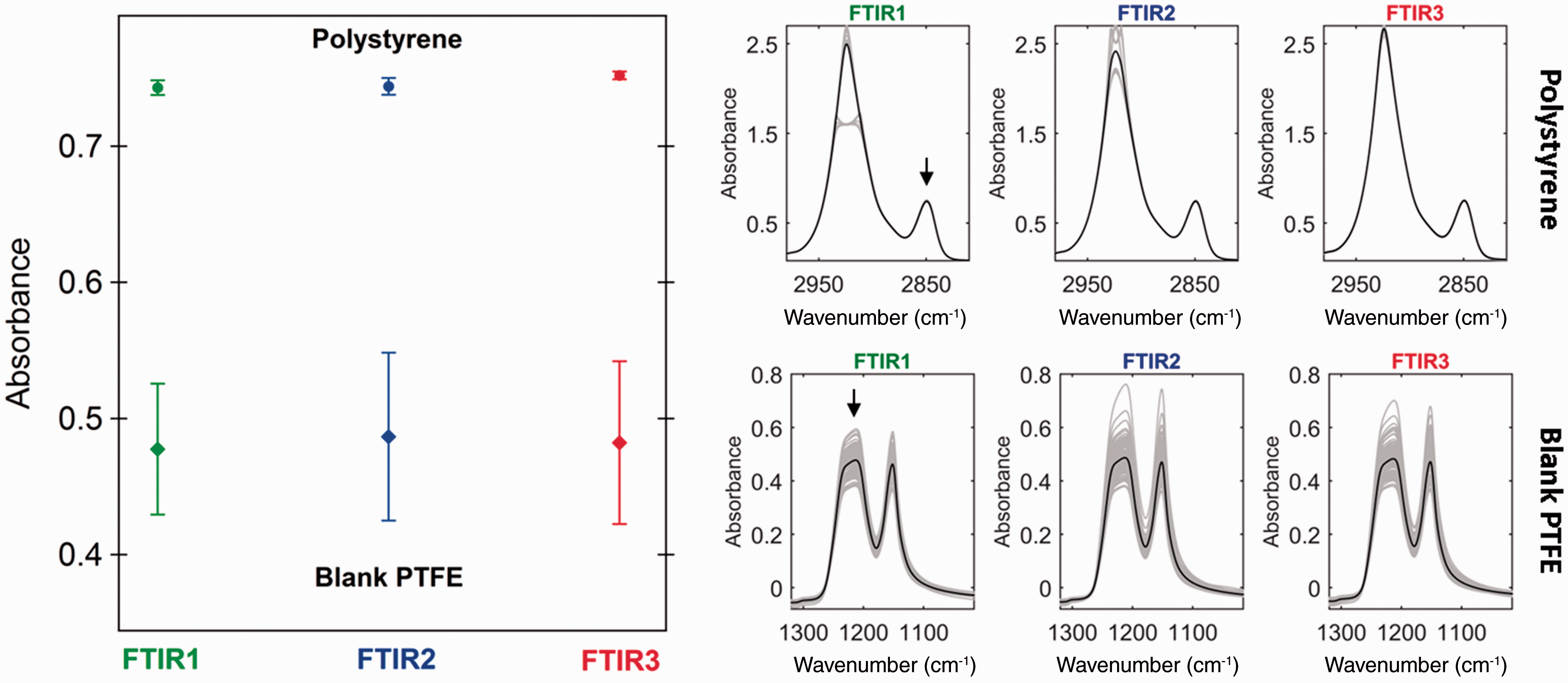

To better evaluate the extent of spectral dissimilarities in the case of filter samples, a similar analysis was conducted on the 1210 cm⁻¹ peak from blank PTFE filters. The PTFE signal in the range 1320–1000 cm⁻¹ is shown in Fig. 1 for all three spectrometers. Compared with polystyrene, the distribution of blank PTFE absorbance values for FTIR1 (0.477 ± 0.048 a.u), FTIR2 (0.487 ± 0.062 a.u), and FTIR3 (0.482 ± 0.060 a.u) is characterized by a larger standard deviation. Significance testing indicates no statistical differences between FTIR2 and FTIR3 blank PTFE absorbance values, suggesting that variability in the observed polystyrene signal is solely attributed to random error. On the other hand, comparing blank PTFE distributions between FTIR1 and FTIR2 or between FTIR1 and FTIR3 reveals statistically significant differences indicating that differences are not just due to random error but also to instrumental or experimental error. The low signal repeatability among filter blanks is mainly attributed to the combination of path length differences and non-uniformity in PTFE fiber morphology,⁴¹ both resulting in a broad distribution of unique optical properties within the same filter and between filters. The substantially larger variation in blank PTFE signal compared to polystyrene leads to the conclusion that spectral dissimilarities across spectrometers are primarily driven by inter-filter variability rather than instrumental factors.

The low repeatability of PTFE signal and its impact on the spectral response of ambient samples is highlighted in Fig. 2a by comparing the FT-IR spectrum of an IMPROVE sample (Wichita Mountains, Oklahoma) collected on all three instruments. The spectral region below 1300 cm⁻¹ is characterized by a collection of sharp and highly absorbing peaks ascribed to the various C–F stretching modes of PTFE.^42,43 Beyond this range, the spectrum features a light-scattering induced sloping baseline as well as a series of low absorbing IR bands at 1720 cm⁻¹, 2844 cm⁻¹, 2911 cm⁻¹, and 3050–3340 cm⁻¹ associated with the IR fingerprints of organic functional groups (FG). The relatively weak absorbance of FG compared with the magnitude of a blank filter (Fig. 2, inset) indicates that PTFE account for the vast majority of the measured signal. Beside minor variations in relative intensity, more pronounced at the higher end of the spectra where scattering prevails, visual inspection of the raw spectra does not reveal any major dissimilarity. Similar comparison based on second derivative spectra confirms the absence of either spectral or intensity shifts, outside of spectral regions featuring water vapor and PTFE contributions (Section 5, Supplemental Material). A more detailed picture of spectral dissimilarities across instruments is obtained by subtracting the spectrum acquired on FTIR1 from the signal measured on FTIR2 and FTIR3. The resulting difference spectra, reported in Fig. 2b, capture information about the nature of spectral differences involved in the signal of ambient samples. Based on the shape and magnitude of the difference spectra, two conclusions can be drawn. First, even though spectral dissimilarities exist across instruments, their respective intensity remain small compared to the raw signal (note the 1000-fold decrease in scale between Fig. 2a and 2b). Second, most of the spectral differences such as the intensity offset and the peak structure at 1200 cm⁻¹ are attributed to PTFE-related factors. Notably, the change in PTFE signal observed across spectrometers for the same ambient sample is induced by the non-uniform density of the filter (Section 6, Supplemental Material). From Fig. 2b, it is worth noting that dissimilarities of lower magnitude can also be spotted such as the signature of carbon dioxide (near 2360 cm⁻¹), water vapor (3500–4000 cm⁻¹, 1540–1800 cm⁻¹), and a trace of volatile organic carbon (VOC, 2900 cm⁻¹).⁴⁴ In single-beam FT-IR studies, minimizing gas-phase absorption is commonly achieved by collecting an empty chamber background before each measurement. In the context of large monitoring networks such as IMPROVE, however, backgrounds are collected hourly to reduce analysis time and accommodate high sample throughput which might cause small fluctuations in water vapor, CO₂, and VOC regions on the measured spectrum. Improving the purge efficiency by using the small volume house-built chamber helps to minimize signal contributions of gas-phase interferents relative to other sample-specific variations (i.e., PTFE).

Figure 2.

(a) Raw and (b) difference FT-IR spectra of the Wichita Mountains, Oklahoma, ambient sample measured on all three spectrometers. Differential spectra are obtained by subtracting both FTIR2 and FTIR3 spectra with the signal collected on FTIR1. Insert representing a blank filter is displayed for the sake of comparison.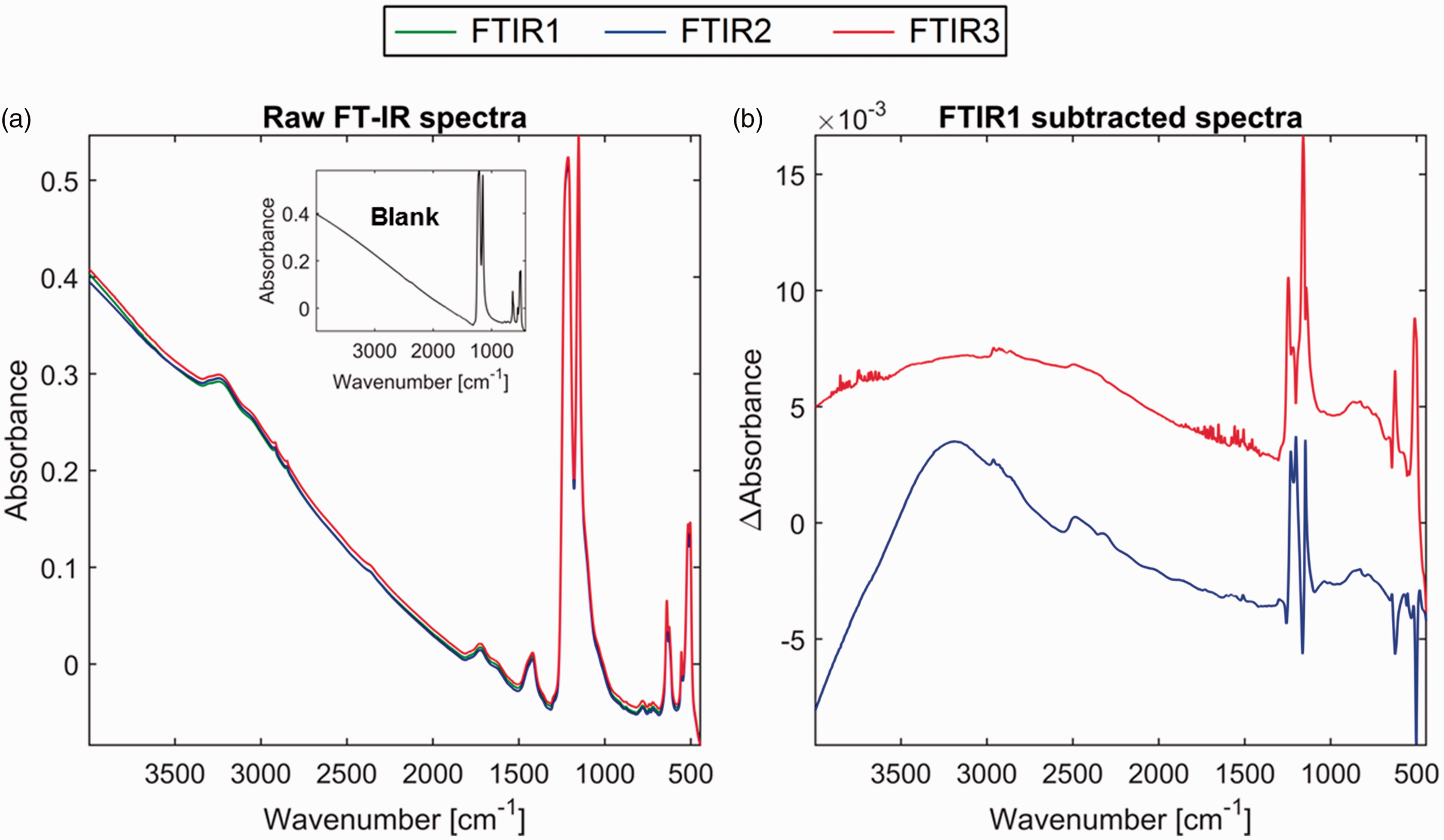

In summary, the strict control of key environmental and instrumental parameters minimizes inter-instrument deviations in spectral response between the three spectrometers. The sources of spectral discrepancies observed in PM filter samples are primarily attributed to PTFE contributions and to a lesser extend to the presence of gas-phase interferents inside the sample compartment.

Impact of Spectral Dissimilarities on Organic Carbon and Elemental Carbon Prediction

To address the performance of OC and EC predictions given the presence of minor inter-instruments spectral dissimilarities, a series of calibration models are developed and validated based on the set of 793 ambient samples introduced in the Data Analysis section. The latter samples, analyzed on both FTIR1 and FTIR2, are stratified into calibration and test sets using a two-thirds (n = 530) and one-third (n = 263) ratio, respectively. First, separate calibrations are developed on each FT-IR system from the set of 530 samples collected within the same instrument. Then, model evaluation is performed following two specific scenarios: (1) validation using the 263 ambient spectra collected on the same instrument; or (2) validation using the 263 ambient spectra acquired on the other instrument. Performance metrics associated with every instrument–scenario combination are reported in Table 1.

Table I.

Comparison of OC and EC model performance between FTIR1 and FTIR2 for scenarios (1) and (2), figures of merit are computed from test set FT-IR spectra (n = 263).

	Calibration	Test	PLS components	R²	RMSEP (µg)	Bias (µg)	Error (µg)	Norm error (%)	MDL (µg)
OC (1)	FTIR1	FTIR1	18	0.97	5.9	0.12	2.98	11.4	3.3
OC (1)	FTIR2	FTIR2	17	0.97	6.0	0.41	3.03	12.9	6.7
OC (2)	FTIR1	FTIR2	18	0.97	5.9	0.01	3.01	13.3	4.8
OC (2)	FTIR2	FTIR1	17	0.97	6.3	0.46	3.20	13.5	5.4
EC (1)	FTIR1	FTIR1	30	0.92	1.7	0.01	0.86	34.4	2.5
EC (1)	FTIR2	FTIR2	32	0.91	1.8	0.12	0.81	34.5	1.8
EC (2)	FTIR1	FTIR2	30	0.91	1.8	0.05	0.89	33.6	1.9
EC (2)	FTIR2	FTIR1	32	0.92	1.7	0.12	0.87	36.4	2.7

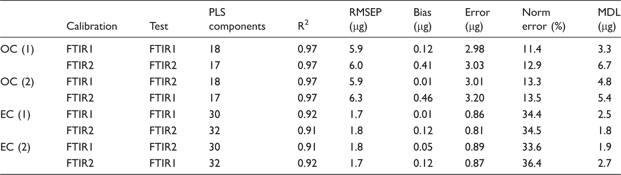
To prevent subjectivity in the assessment of significant differences between models developed on FTIR1 and FTIR2, the ratio of the squared RMSEP values obtained for each model was computed and compared to the critical value of a two-sided F-test at the 95% confidence level.^45,46 Since all calculated ratios fall below the critical value F_{(n = 262, n = 262, 0.95)} = 1.275, OC and EC models developed separately on each instrument are not considered statistically different. Furthermore, swapping models between spectrometers (2) does not introduce significant differences in prediction metrics with the exception of a slight increase in normalized error. Although model performances are considered equivalent, the impact of spectral dissimilarities between instruments can still be observed in the form of a higher bias and MDL on FTIR2 as well as a slightly different number of PLS components. Despite the apparent variability in MDL, values remain consistent with the ones reported in previous works.^9,47

Considering that inter-instrument spectral dissimilarities are predominantly influenced by filter anisotropic properties, maintaining high-quality predictions supposes the selection of an appropriate subset of calibration samples which is representative of both PM composition and optical properties of the substrate experienced in test samples. In Table 1, the statistical equivalence between the performance of the models suggests that the size of the calibration set is adequate. However, it is likely that a different number of calibration samples or a different samples combination could achieve equivalent prediction performance. To estimate the optimal (i.e., minimal) size of the calibration set required to maintain high-quality predictions, the number of calibration samples N_cal was gradually decreased from 530 to 57 while keeping the number of blanks constant (n = 34). For each calibration set, a PLS model was generated and validated using the same test set as in Table 1 (n = 263). In Fig. 3, variations in model performance as function of N_cal are shown for the case of OC prediction metrics developed from scenario (1). Complementary studies associated with scenario (2) and EC predictions are given in the Supplemental Material (Section 7). No significant degradation in prediction is observed until N_cal drops by more than half of its initial size (n = 244). Between 530 and 244 calibration samples, nearly identical metrics are reported for both OC scenarios with the exception of a consistently higher bias on FTIR2 (≈0.5 µg) suggesting slightly overestimated OC concentrations compared with FTIR1. However, the magnitude of such a bias is lower than the 95% confidence interval (CI) of test set blank predicted concentrations ( ± 0.9 µg) and could thus be considered negligible. As N_cal decreases from 244 to 140, a moderate deterioration in prediction metrics might suggest that calibration samples are no longer representative of the whole distribution in PTFE and PM composition of test set samples. Further reduction in the number of samples yields increased error with prediction metrics no longer matching between the two spectrometers. The R² and RMSEP plots in Fig. S7-2 (Supplemental Material) suggest similar conclusions for EC prediction.

Figure 3.

Inter-instrument comparison of OC prediction metrics based on scenario (1) as function of the number of samples N_cal included in the calibration. Reported performance are derived from test spectra (n = 263) collected on the same instrument used to analyze calibration samples. Models are developed and evaluated with samples from the year 2015.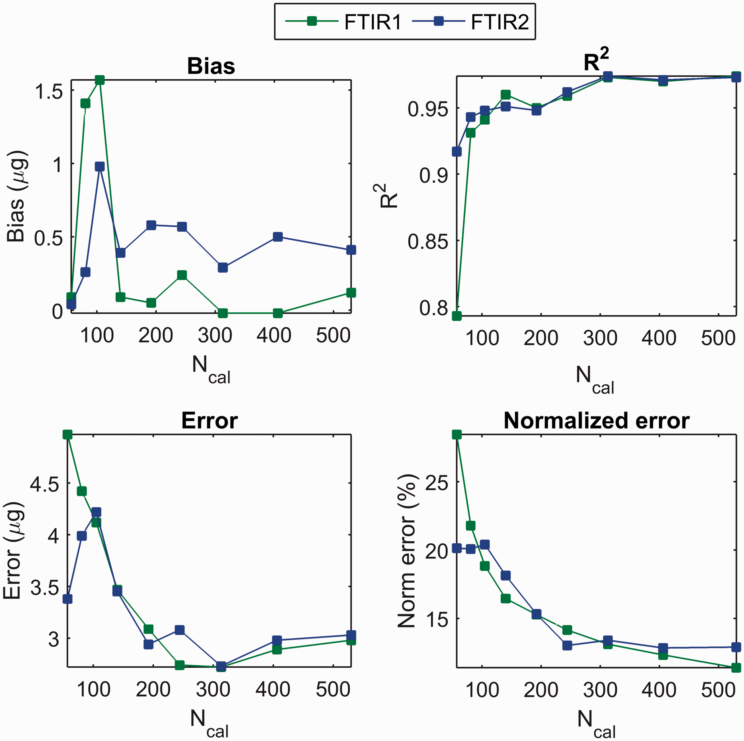

To assess the extent of PTFE variability between test and calibration samples, distribution parameters (e.g., mean absorbance) of the PTFE peak at 1210 cm⁻¹ are derived from the raw spectra (Fig. S7-3, Supplemental Material). For N_cal values > 250, PTFE distribution parameters derived from calibration and test spectra are nearly identical and therefore do not influence the prediction quality other than a negligible bias. However, lower N_cal values are characterized by a divergence in PTFE distribution parameters between calibration and test spectra which likely contributes to the drop in prediction quality seen in Fig. 3. In addition to the lack of representativeness of PTFE distribution in test samples, the progressive degradation of OC prediction as N_cal decreases is also attributed to unmatched PM composition between calibration and test samples. According to Fig. S7-3, at least 300 samples are required in the calibration in order to efficiently diminish the impact of PTFE signal variability on model performance.

Based on the results from the two first scenarios, the variability in PTFE signal appears to have little to no influence on OC and EC prediction as long as the calibration set is representative of both PTFE and PM composition in test samples. The fact that calibration models built on either instrument predict equivalent concentrations without resorting to sophisticated calibration transfer strategies is attributed to two factors. One is the strict control of water vapor and carbon dioxide concentrations, detector temperature, sample position relative to the IR beam, and room conditions which enable the instruments to provide similar responses. The second is the capability of PLS to reduce the remaining sources of variability interfering with OC or EC prediction (i.e., PTFE).

Because maintaining multiple calibration models over time is generally not suitable from a long-term perspective, and considering that models developed separately on each instrument are statistically equivalent, it appears that either calibration can be selected as part of a routine measurement procedure. However, neither model accounts for the specific spectral response of both instruments as indicated by the difference in bias reported in Table 1 and in Fig. 3 for FTIR1 and FTIR2. To ensure that instrument specific differences, while small, are accounted for, an instrument-agnostic calibration model, often referred to as a hybrid model,⁴⁸ is introduced. The hybrid model is presented in a third scenario (3) by using spectra acquired on both spectrometers within a single calibration set. To ensure that the number of samples, the distribution of sites, and the sample composition remain the same as in Table 1, only samples whose array index features odd numbers on FTIR1 and even numbers on FTIR2 were included in the calibration. Performance associated with the third scenario, reported in Table II, was evaluated from the same set of test spectra used previously on scenarios (1) and (2). As in Table 1, the significance testing of the RMSEP values do not exceed the critical value F_{(n = 262, n = 262, 0.95)} = 1.275, indicating that the hybrid model predicts OC and EC concentrations equally well on both spectrometers. In general, similar or slightly improved OC prediction metrics are reported compared with models built on a single instrument while similar or slightly worse prediction metrics can be claimed for EC. Because EC has low IR activity,⁴⁹ the corresponding hybrid model is more prone to overfitting due to the presence of low-magnitude spectral interferents. In particular, difference in water vapor and carbon dioxide content from one instrument to another is assumed to be the main factor explaining the decrease in EC prediction. Nonetheless, the overall performance by the hybrid model is considered satisfactory for providing robust predictions independent of the instrument. Additional benefit of the hybrid model compared with the other two scenarios can be inferred from the absence of significant bias between the two spectrometers. The larger bias previously reported for FTIR2 is corrected for by simply developing a common set of regression coefficients considering the characteristics of both instruments. The third FT-IR instrument will be evaluated for inclusion into a hybrid calibration model using spectra from all three instruments in future studies.

Table II.

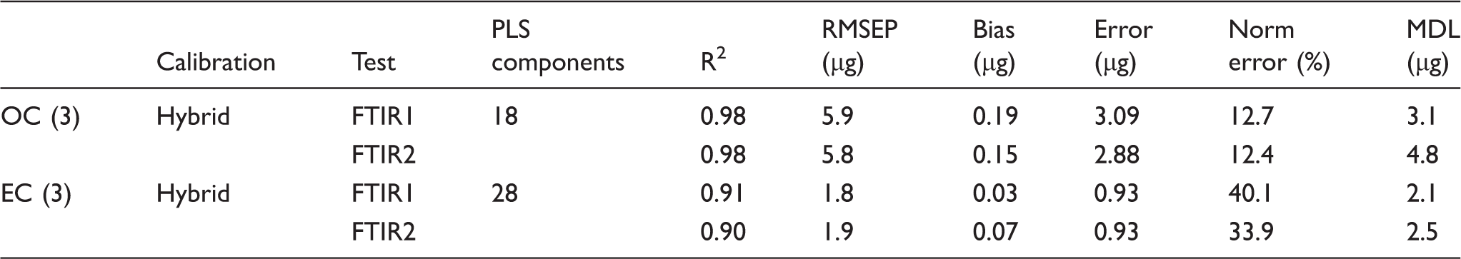
Comparison of OC and EC hybrid model performance between FTIR1 and FTIR2 for scenario (3), figures of merit are computed from test set FT-IR spectra (n = 263).

	Calibration	Test	PLS components	R²	RMSEP (µg)	Bias (µg)	Error (µg)	Norm error (%)	MDL (µg)
OC (3)	Hybrid	FTIR1	18	0.98	5.9	0.19	3.09	12.7	3.1
OC (3)	Hybrid	FTIR2	18	0.98	5.8	0.15	2.88	12.4	4.8
EC (3)	Hybrid	FTIR1	28	0.91	1.8	0.03	0.93	40.1	2.1
EC (3)	Hybrid	FTIR2	28	0.90	1.9	0.07	0.93	33.9	2.5

Repeatability and Long-Term Stability Assessment

Instrument stability within a short time frame, typically on the order of a few hours, is first addressed by considering daily duplicate measurements collected once or twice per day on each instrument. After subjecting all replicate spectra to the hybrid models, the subsequent predicted concentrations for each sample pair is used to compute instrument precision, a reliable estimate of measurement repeatability, according to Eq. 1. While equivalent precision values are achieved on FTIR1 (0.79 µg) and FTIR2 (0.75 µg) for OC, EC results suggest that FTIR2 provides more robust measurement repeatability than FTIR1 with precision values of 0.26 µg (FTIR2) and 0.73 µg (FTIR1). Although slightly elevated, calculated precisions are of the same order of magnitude as the 95% CI of test set blank predicted OC ( ± 0.70 µg) and EC ( ± 0.42 µg) concentrations. Given the narrow gap between precision and the 95% CI values, the stability of both spectrometers over a short period of time is considered satisfactory and justifies the choice to collect backgrounds hourly.

Through variations introduced by environmental conditions or characteristics of the instrument, a change in spectral response over time is a common occurrence in spectroscopic systems. Therefore, monitoring instrument stability is required to ensure the validity of the hybrid model over time, highlight any new potential sources of spectral variations affecting model performance, and foresee situations where a full recalibration may be required. In an attempt to identify long-term drifts in instrument response, we refer to the set of four reference samples selected for this evaluation. Unlike IMPROVE ambient samples, reference filters are always measured at a fixed orientation to minimize the impact of filter anisotropic properties and emphasize spectral variations induced by the instruments. Predicted concentrations, calculated weekly for each reference sample based on the OC hybrid model, are used to develop a group of time series plots displayed in Fig. 4. The series is characterized by (local) non-periodic oscillations in predicted concentrations attributed to minor changes in background properties over time induced by either environmental- or instrument-related perturbations. To assess the extent of those variations, the median OC concentration is computed based on the first month of data collection on all three spectrometers. Intervals corresponding to ±5% (dotted lines) and ±10% (straight lines) variations around the median predicted concentration are then considered for reference ambient samples while only the median predicted concentration is displayed for blank reference filters (dotted lines). Almost 90% of the predicted concentrations of reference ambient samples measured over a 2.5-year period for FTIR1 and FTIR2 and over an eight-month period for FTIR3 are within the ±5% of the initial concentration while about 10% lie in the ±5–10% interval. The absence of clear drift in predicted standard OC concentrations over an extended period of time highlights the relative stability of the spectral response on all three FT-IR systems. Similar conclusions can be drawn in the case of EC predictions (data not shown).

Figure 4.

Concentrations time series of four reference samples predicted by the hybrid OC model initially developed for the year 2015. The x-axis corresponds to the date when the analysis was performed. Dashed and solid lines for reference ambient samples indicate the ±5% and ±10% error intervals based on the median OC concentration calculated by averaging the first month of data collection for all three instruments. Dashed lines for reference blank filters represent the median concentration.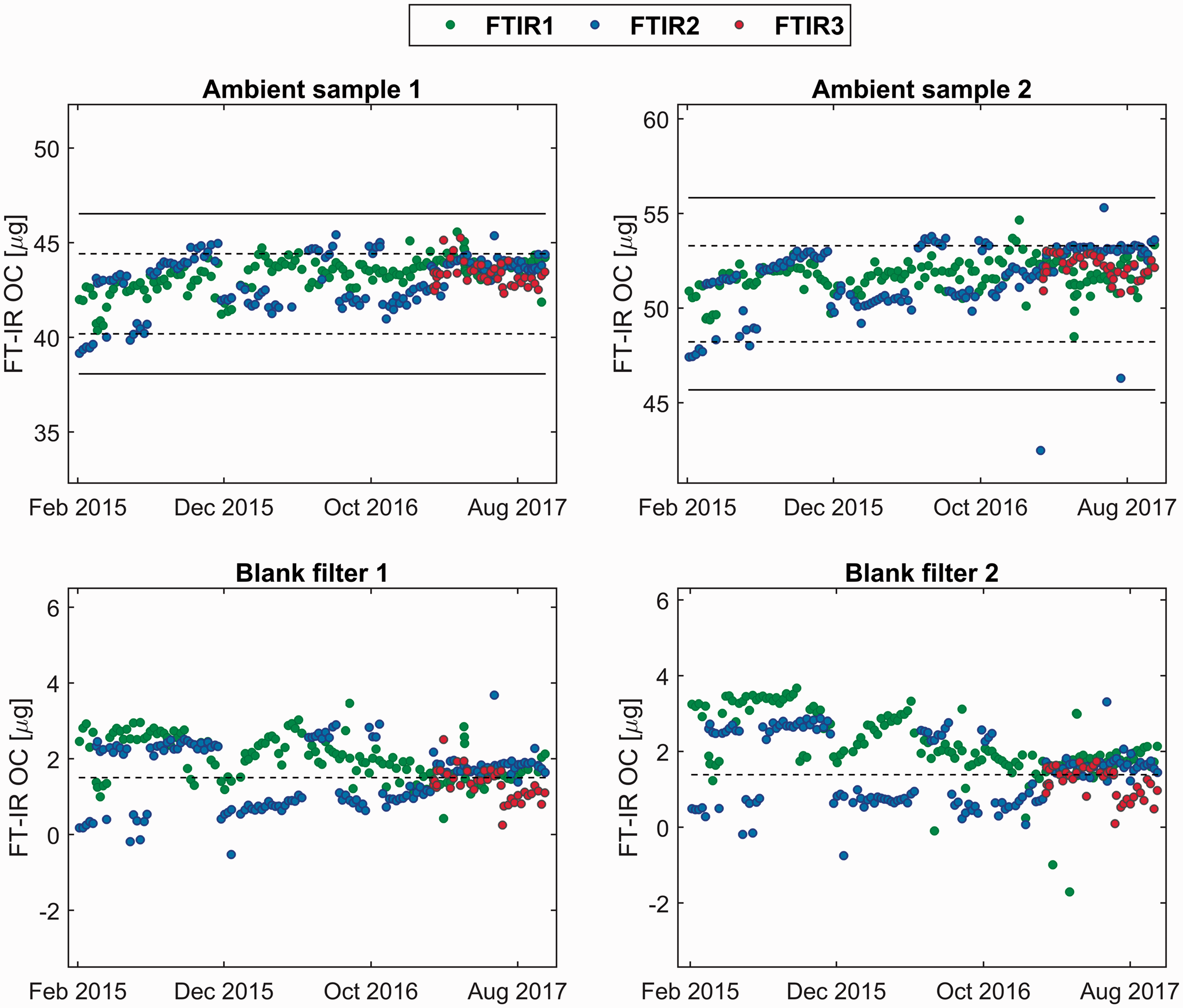

Although reference samples provide a reliable screening tool to monitor instrument stability over time, their composition is not necessarily representative of the PM distribution experienced in network ambient samples. To address this issue, a similar study was conducted using 2078 FT-IR spectra of ambient PM samples measured on both FTIR1 and FTIR2 over the same three-year time period. For each year of spectra collection, predicted concentrations achieved on FTIR2 are regressed against their FTIR1 counterpart and a simple ordinary least squares regression procedure is employed to derive slope and intercept parameters. Percentile-based bootstrapped CIs are then developed to test whether or not the calculated slope and intercept are significantly different from one and zero, respectively.⁵⁰ In this study, we rely on 95% CIs computed from a series of 1000 bootstrap replicates for each metric. Yearly slope, intercept, and their respective 95% CIs derived for OC prediction on the FTIR2–FTIR1 instrument pair are illustrated in Fig. 5.

Figure 5.

Time-dependent slopes (left) and intercepts (right) derived from test set OC predicted concentrations on the FTIR2–FTIR1 instrument pair, uncertainty of each metric is evaluated by developing 95% CIs from 1000 bootstrap replicates.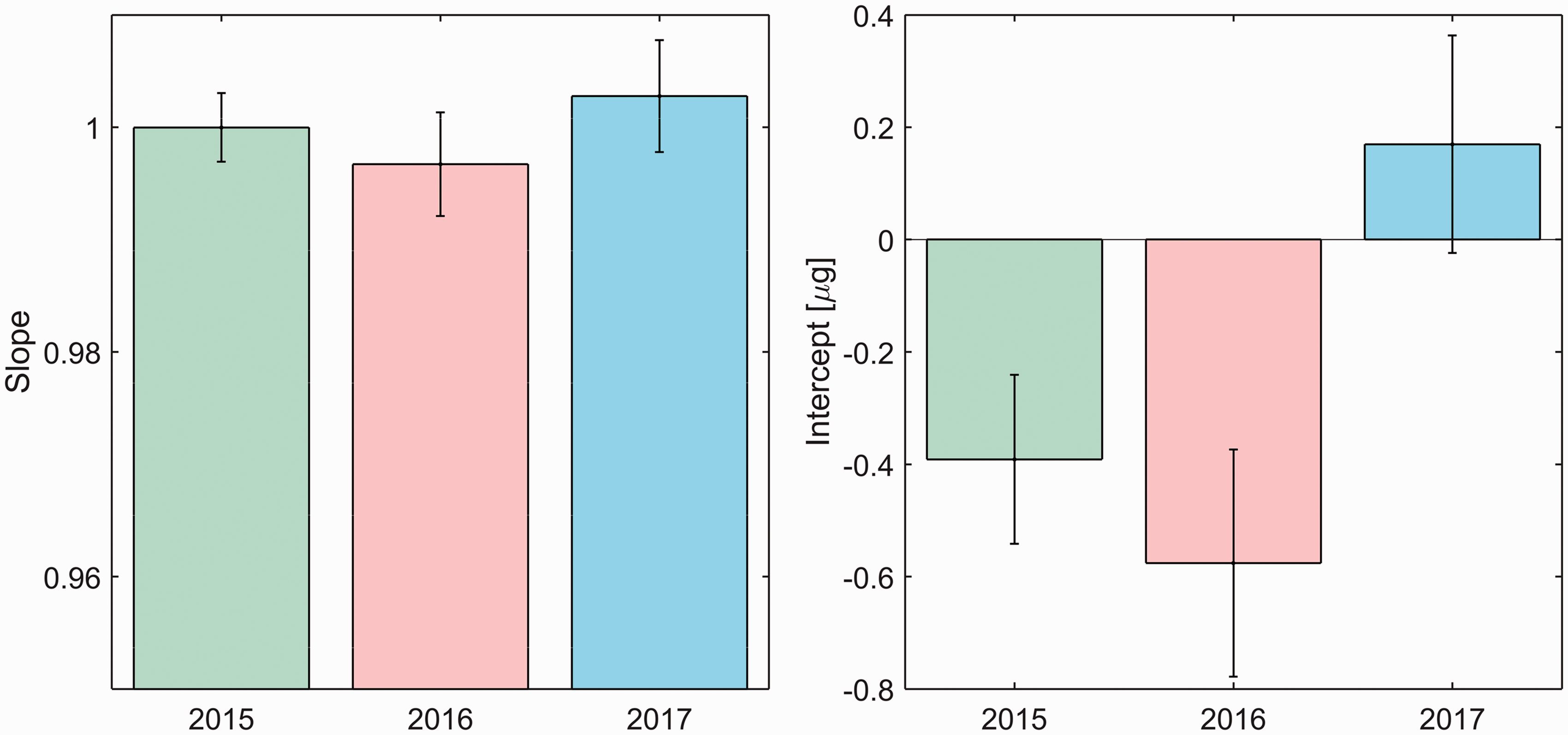

Figure 5 shows that the hybrid model still provides acceptable predictions for both 2016 and 2017 IMPROVE samples. This corroborates the findings of Reggente et al. who showed that a single-instrument calibration model can be extended to samples collected and analyzed in a subsequent year.⁴⁷ Notably, slope-associated CIs reveal no significant differences in cross-instrument predictions between consecutive years. The high quality of the regression is suggested by the fact that none of the calculated slopes are statistically different than one. The presence of non-zero intercepts, however, discloses a low magnitude bias between the predictions achieved on FTIR1 and FTIR2. While the years 2015 and 2016 are both characterized by negative intercepts, significantly different from zero, the year 2017 features a positive intercept not statistically different from zero. Relative to the year 2015, the moderate increase in the 2016 intercept is tentatively attributed to the transfer of the instruments to a new laboratory room. However, the change in intercept for 2017 data is not yet clearly associated with any known sources of interference but the increase in predicted reference concentrations on FTIR2 (Fig. 4) in early 2017 suggests an instrumental drift. As the intercepts remain below the MDL (Table II), the performance of the OC hybrid model extended to the years 2016 and 2017 are nonetheless considered satisfactory. Similar results are observed for the EC hybrid model (Fig. S8-1, Supplemental Material) for which a significant gap between 2016 (0.14 µg) and 2017 (–0.94 µg) intercepts is also observed. Such a difference, larger than the precision values reported above, pinpoints the limitation and sensitivity of the hybrid EC model to variations in experimental conditions.

Finally, instrument pairs involving the new FTIR3 system were investigated for the restricted 2017 time period. While FTIR3–FTIR1 and FTIR3–FTIR2 pairs provide equivalent OC predictions (Fig. S7-2), different results are reported for EC with the absence of overlap in the 95% confidence intercept interval (Section 8, Supplemental Material). Despite the elevated intercept values, instrument or model recalibration is not suggested as the intercept between instrument-pairs does not exceed EC MDL values in Table II.

Conclusion

This paper describes the strategy behind the development of a robust, low maintenance, calibration model applicable across multiple FT-IR instruments and multiple years. The need for advanced calibration transfer procedures was circumvented by carefully controlling instrumental and environmental parameters in an attempt to minimize dissimilarities in instrument response. After ensuring that all spectrometers are operated under fixed experimental conditions, the remaining sources of spectral variability were attributed to the heterogeneous structural and optical properties of PTFE filters. However, the effects of PTFE interference have little to no influence on OC and EC predicted concentrations as long as calibration samples are representative of the PTFE variability and PM composition in test samples. Instead of building a specific calibration per instrument, hybrid OC and EC calibration models were developed based on ambient IMPROVE spectra collected on each spectrometer. With the exception of a small decrease in EC prediction capability attributed to variations in water vapor and carbon dioxide content inside the sample compartments, hybrid models provide robust and accurate predictions independent of the spectrometer used for data acquisition. The weekly spectral collection of duplicate and standard PM samples indicates both high measurement repeatability and long-term stability of the response of the instruments. Extending hybrid OC and EC models, developed for the year 2015, to the prediction of ambient PM samples collected in the two subsequent years does not produce significant changes in prediction metrics further indicating that the proposed hybrid calibration models are suitable for OC and EC prediction in network operations.

Supplemental Material

Supplemental material for Long-Term Strategy for Assessing Carbonaceous Particulate Matter Concentrations from Multiple Fourier Transform Infrared (FT-IR) Instruments: Influence of Spectral Dissimilarities on Multivariate Calibration Performance

Supplemental Material for Long-Term Strategy for Assessing Carbonaceous Particulate Matter Concentrations from Multiple Fourier Transform Infrared (FT-IR) Instruments: Influence of Spectral Dissimilarities on Multivariate Calibration Performance by Bruno Debus, Satoshi Takahama, Andrew T. Weakley, Kelsey Seibert and Ann M. Dillner in Applied Spectroscopy

Footnotes

Acknowledgments

The authors would like to acknowledge all of the UC Davis undergraduate students who collected FT-IR spectra and Nikunj Dudani and Audrey Atherton of EPFL for their assistance with the chamber testing protocol.

Conflict of Interest

The authors report there are no conflicts of interest.

Funding

The authors acknowledge funding from the National Park Service in cooperation with the Environmental Protection Agency (P11AC91045) as well as EPFL funding.

Supplemental Material

All supplemental material mentioned in the text, consisting of Figs. S1–S8, is available in the online version of the journal.

References

Bauer

Nieuwoudt

Bauer

F.F.

Kossmann

et al.

“FTIR Spectroscopy for Grape and Wine Analysis”. Anal. Chem. 2008. 80(5): 1371–1379.

Cassani

Santos

Gerbino

Del Rosario Moreira

et al.

“A Combined Approach of Infrared Spectroscopy and Multivariate Analysis for the Simultaneous Determination of Sugars and Fructans in Strawberry Juices During Storage”. J. Food Sci. 2017. 83(3): 631–638.

Yousefinejad

Aalizadeh

Honarasa

“Application of ATR-FTIR Spectroscopy and Chemometrics for the Discrimination of Furnace Oil, Gas Oil and Mazut Oil”. Anal. Methods. 2016. 8(23): 4640–4647.

Bunaciu

A.A.

Aboul-Enein

H.Y.

Fleschin

“Application of Fourier Transform Infrared Spectrophotometry in Pharmaceutical Drugs Analysis”. Appl. Spectrosc. Rev. 2010. 45(3): 206–219.

Koch

Posch

A.E.

Goicoechea

H.C.

Herwig

et al.

“Multi-Analyte Quantification in Bioprocesses by Fourier-Transform-Infrared Spectroscopy by Partial Least Squares Regression and Multivariate Curve Resolution”. Anal. Chim. Acta. 2014. 807: 103–110.

Chang

P.E.P.

Yang

J.C.R.

Den

C.F.

“Characterizing and Locating Air Pollution Sources in A Complex Industrial District Using Optical Remote Sensing Technology and Multivariate Statistical Modeling”. Environ. Sci. Pollut. Res. 2014. 21(18): 10852–10866.

Russell

L.M.

“Aerosol Organic-Mass to Organic-Carbon Ratio Measurements”. Environ. Sci. Technol. 2003. 37(13): 2982–2987.

Wold

Sjöström

Eriksson

“PLS-Regression: A Basic Tool of Chemometrics”. Chemom. Intell. Lab. Syst. 2001. 58(2): 109–130.

Dillner

A.M.

Takahama

“Predicting Ambient Aerosol Thermal-Optical Reflectance (TOR) Measurements from Infrared Spectra: Organic Carbon”. Atmos. Meas. Tech. 2015. 8(3): 1097–1109.

10.

Dillner

A.M.

Takahama

“Predicting Ambient Aerosol Thermal-Optical Reflectance Measurements from Infrared Spectra: Elemental Carbon”. Atmos. Meas. Tech. 2015. 8(10): 4013–4023.

11.

Coury

Dillner

A.M.

“A Method to Quantify Organic Functional Groups and Inorganic Compounds in Ambient Aerosols Using Attenuated Total Reflectance FTIR Spectroscopy and Multivariate Chemometric Techniques”. Atmos. Environ. 2008. 42(23): 5923–5932.

12.

Ruthenburg

T.C.

Perlin

P.C.

Liu

McDade

C.E.

et al.

“Determination of Organic Matter and Organic Matter to Organic Carbon Ratios by Infrared Spectroscopy with Application to Selected Sites in the IMPROVE Network”. Atmos. Environ. 2014. 86(Suppl. C): 47–57.

13.

George

K.M.

Ruthenburg

T.C.

Smith

et al.

“FT-IR Quantification of the Carbonyl Functional Group in Aqueous-Phase Secondary Organic Aerosol from Phenols”. Atmos. Environ. 2015. 100(Suppl. C): 230–237.

14.

Solomon

P.A.

Costantini

Grahame

T.J.

Gerlofs-Nijland

M.E.

et al.

“Air Pollution and Health: Bridging the Gap from Sources to Health Outcomes: Conference Summary”. Air Qual. Atmos. Health. 2012. 5(1): 9–62.

15.

Zhao

Zhang

Jiang

et al.

“Effects of Atmospheric Transport and Trade on Air Pollution Mortality in China”. Atmos. Chem. Phys. 2017. 17(17): 10367–10381.

16.

Glotfelty

Zhang

Karamchandani

Streets

D.G.

“Will the Role of Intercontinental Transport Change in A Changing Climate?” Atmos. Chem. Phys. 2014. 14(17): 9379–9402.

17.

Y. Liu, Z. Liu, R. Maghirang, E. Santos, et al. “Apportionment of Visibility Degradation to Sources of PM2.5 in Rural and Urban Kansas”. Paper presented at 2017 ASABE Annual International Meeting, Spokane, Washington; July 16–19, 2017.

18.

Watson

J.G.

“Visibility: Science and Regulation”. J. Air Waste Manag. Assoc. 2002. 52(6): 628–713.

19.

Jimenez

J.L.

Canagaratna

M.R.

Donahue

N.M.

Prevot

A.S.H.

et al.

“Evolution of Organic Aerosols in the Atmosphere”. Science. 2009. 326(5959): 1525–1529.

20.

Hamilton

J.F.

Webb

P.J.

Lewis

A.C.

Hopkins

J.R.

et al.

“Partially Oxidised Organic Components in Urban Aerosol Using GCXGC-TOF/MS”. Atmos. Chem. Phys. 2004. 4(5): 1279–1290.

21.

Tao

Chin

“Impact of Transpacific Aerosol on Air Quality Over the United States: A Perspective from Aerosol–Cloud–Radiation Interactions”. Atmos. Environ. 2016. 125(Part A): 48–60.

22.

Snider

Weagle

C.L.

Martin

R.V.

Van Donkelaar

et al.

“SPARTAN: A Global Network to Evaluate and Enhance Satellite-Based Estimates of Ground-Level Particulate Matter for Global Health Applications”. Atmos. Meas. Tech. 2015. 8(1): 505–521.

23.

Tørseth

Aas

Breivik

Fjæraa

A.M.

et al.

“Introduction to the European Monitoring and Evaluation Programme (EMEP) and Observed Atmospheric Composition Change During 1972–2009”. Atmos. Chem. Phys. 2012. 12(12): 5447–5481.

24.

Malm

W.C.

Schichtel

B.A.

Pitchford

M.L.

Ashbaugh

L.L.

et al.

“Spatial and Monthly Trends in Speciated Fine Particle Concentration in the United States”. J. Geophys. Res. 2004. 109(D3): D03306.

25.

Solomon

P.A.

Crumpler

Flanagan

J.B.

Jayanty

R.K.M.

et al.

“U.S. National PM2.5 Chemical Speciation Monitoring Networks—CSN and IMPROVE: Description of Networks”. J. Air Waste Manag. Assoc. 2014. 64(12): 1410–1438.

26.

Dambergs

R.G.

Mercurio

M.D.

Kassara

Cozzolino

et al.

“Rapid Measurement of Methyl Cellulose Precipitable Tannins Using Ultraviolet Spectroscopy with Chemometrics: Application to Red Wine and Inter-Laboratory Calibration Transfer”. Appl. Spectrosc. 2012. 66(6): 656–664.

27.

Morgan

C.L.S.

Grunwald

Brown

D.J.

et al.

“Comparison of Soil Reflectance Spectra and Calibration Models Obtained Using Multiple Spectrometers”. Geoderma. 2011. 161(3–4): 202–211.

28.

Grelet

Fernández Pierna

J.A.

Dardenne

Baeten

et al.

“Standardization of Milk Mid-Infrared Spectra from A European Dairy Network”. J. Dairy Sci. 2015. 98(4): 2150–2160.

29.

Sohn

Barton Ii

F.E.

Himmelsbach

D.S.

“Transfer of Near-Infrared Calibration Model for Determining Fiber Content in Flax: Effects of Transfer Samples and Standardization Procedure”. Appl. Spectrosc. 2007. 61(4): 414–418.

30.

Sales

Callao

M.P.

Rius

F.X.

“Multivariate Standardization Techniques Using UV–Vis Data”. Chemom. Intell. Lab. Syst. 1997. 38(1): 63–73.

31.

Workman

J.J.

Jr . “A Review of Calibration Transfer Practices and Instrument Differences in Spectroscopy”. Appl. Spectrosc. 2018. 72(3): 340–365.

32.

Feudale

R.N.

Woody

N.A.

Tan

Myles

A.J.

et al.

“Transfer of Multivariate Calibration Models: A Review”. Chemom. Intell. Lab. Syst. 2002. 64(2): 181–192.

33.

Swierenga

Haanstra

W.G.

De Weijer

A.P.

Buydens

L.M.C.

“Comparison of Two Different Approaches Toward Model Transferability in NIR Spectroscopy”. Appl. Spectrosc. 1998. 52(1): 7–16.

34.

Bouveresse

Hartmann

Massart

D.L.

Last

I.R.

et al.

“Standardization of Near-Infrared Spectrometric Instruments”. Anal. Chem. 1996. 68(6): 982–990.

35.

De Noord

O.E.

“Multivariate Calibration Standardization”. Chemom. Intell. Lab. Syst. 1994. 25(2): 85–97.

36.

Adhihetty

I.S.

McGuire

J.A.

Wangmaneerat

Niemczyk

T.M.

et al.

“Achieving Transferable Multivariate Spectral Calibration Models: Demonstration with Infrared Spectra of Thin-Film Dielectrics on Silicon”. Anal. Chem. 1991. 63(20): 2329–2338.

37.

Kennard

R.W.

Stone

L.A.

“Computer Aided Design of Experiments”. Technometrics. 1969. 11(1): 137–148.

38.

Chow

J.C.

Watson

J.G.

Pritchett

L.C.

Pierson

W.R.

et al.

“The Dri Thermal/Optical Reflectance Carbon Analysis System: Description, Evaluation and Applications in U.S. Air Quality Studies”. Atmos. Environ. Gen. Top. 1993. 27(8): 1185–1201.

39.

Arlot

Celisse

“A Survey of Cross-Validation Procedures for Model Selection”. Stat. Surv. 2010. 4: 40–79.

40.

H.-D.

Q.-S.

Liang

Y.-Z.

“LibPLS: An Integrated Library for Partial Least Squares Regression and Linear Discriminant Analysis”. Chemom. Intell. Lab. Syst. 2018. 176: 34–43.

41.

Quarti

Milani

Castiglioni

“Ab Initio Calculation of the IR Spectrum of PTFE: Helical Symmetry and Defects”. J. Phys. Chem. B. 2013. 117(2): 706–718.

42.

Liang

C.Y.

Krimm

“Infrared Spectra of High Polymers. III. Polytetrafluoroethylene and Polychlorotrifluoroethylene”. J. Chem. Phys. 1956. 25(3): 563–571.

43.

Moynihan

R.E.

“The Molecular Structure of Perfluorocarbon Polymers. Infrared Studies on Polytetrafluoroethylene”. J. Am. Chem. Soc. 1959. 81(5): 1045–1050.

44.

Kim

U.J.

Furtado

C.A.

Liu

Chen

et al.

“Raman and IR Spectroscopy of Chemically Processed Single-Walled Carbon Nanotubes”. J. Am. Chem. Soc. 2005. 127(44): 15437–15445.

45.

Pereira

C.F.

Pimentel

M.F.

Galvão

R.K.H.

Honorato

F.A.

et al.

“A Comparative Study of Calibration Transfer Methods for Determination of Gasoline Quality Parameters in Three Different Near Infrared Spectrometers”. Anal. Chim. Acta. 2008. 611(1): 41–47.

46.

Gryniewicz-Ruzicka

C.M.

Arzhantsev

Pelster

L.N.

Westenberger

B.J.

et al.

“Multivariate Calibration and Instrument Standardization for the Rapid Detection of Diethylene Glycol in Glycerin by Raman Spectroscopy”. Appl. Spectrosc. 2011. 65(3): 334–341.

47.

Reggente

Dillner

A.M.

Takahama

“Predicting Ambient Aerosol Thermal-Optical Reflectance (TOR) Measurements from Infrared Spectra: Extending the Predictions to Different Years and Different Sites”. Atmos. Meas. Tech. 2016. 9(2): 441–454.

48.

Ozdemir

Mosley

Williams

“Hybrid Calibration Models: An Alternative to Calibration Transfer”. Appl. Spectrosc. 1998. 52(4): 599–603.

49.

Figueiredo

J.L.

Pereira

M.F.R.

Freitas

M.M.A.

Órfão

J.J.M.

“Modification of the Surface Chemistry of Activated Carbons”. Carbon. 1999. 37(9): 1379–1389.

50.

Efron

Tibshirani

R.J.

An Introduction to the Bootstrap. New York; London: Chapman and Hall, 1993.

Supplementary Material

Please find the following supplemental material available below.

For Open Access articles published under a Creative Commons License, all supplemental material carries the same license as the article it is associated with.

For non-Open Access articles published, all supplemental material carries a non-exclusive license, and permission requests for re-use of supplemental material or any part of supplemental material shall be sent directly to the copyright owner as specified in the copyright notice associated with the article.

0.00 MB

5.17 MB