Optimised Pre-Processing of Raman Spectra for Colorectal Cancer Detection Using High-Performance Computing

Abstract

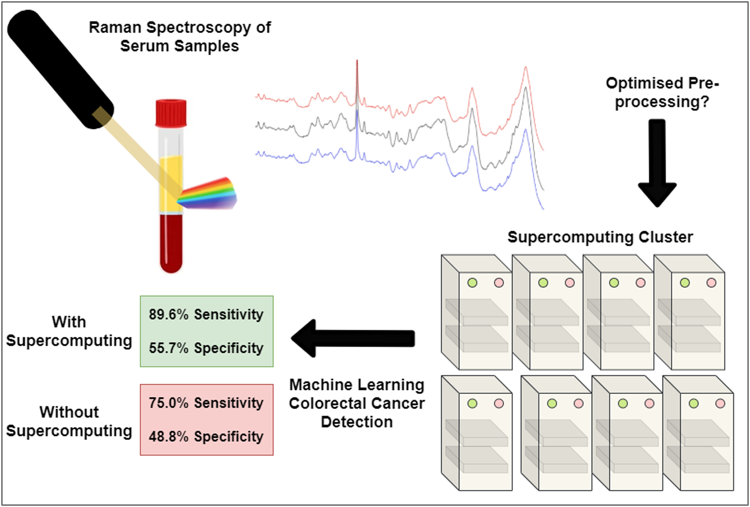
Spectral pre-processing is an essential step in data analysis for biomedical diagnostic applications of Raman spectroscopy, allowing the removal of undesirable spectral contributions that could mask biological information used for diagnosis. However, due to the specificity of pre-processing for a given sample type and the vast number of potential pre-processing combinations, optimisation of pre-processing via a manual “trial and error” format is often time intensive with no guarantee that the chosen method is optimal for the sample type. Here we present the use of high-performance computing (HPC) to trial over 2.4 million pre-processing permutations to demonstrate the optimisation on the pre-processing of human serum Raman spectra for colorectal cancer detection. The effect of varying pre-processing order, using extended multiplicative scatter correction, spectral smoothing, baseline correction, binning and normalization was considered. Permutations were assessed on their ability to detect patients with disease using a random forest (RF) algorithm trained with 102 patients (510 spectra) and independently tested with a set of 439 patients (1317 spectra) in a primary care patient cohort. Optimising via HPC enables improved performance in diagnostic abilities, with sensitivity increasing by 14.6%, specificity increasing by 6.9%, positive predictive value increasing by 3.4%, and negative predictive value increasing by 2.4% when compared to a standard pre-processing optimisation. Ultimate values of these metrics are very important for diagnostic adoption, and once diagnostics demonstrate good accuracy these types of optimisations can make a significant difference to roll-out of a test and demonstrating advantages over existing tests. We also provide tips/recommendations for pre-processing optimisation without the use of HPC. From the HPC permutations, recommendations for appropriate parameter constraints for conducting a more basic pre-processing optimisation are also detailed, thus helping model development for researchers not having access to HPC.

Graphical Abstract

Keywords

Raman spectroscopy high-performance computing cancer biospectroscopy machine learning pre-processing optimisation

Introduction

Raman spectroscopy (RS) offers the ability to obtain the complex structural fingerprint of the molecular constituents in a sample by the inelastic scattering of electromagnetic (EM) radiation.¹ The analysis of biological samples using RS and machine learning algorithms is becoming ever more prevalent, with applications highlighted to analyse bio-fluids,^2–6 tissue samples^7–10 and cells.^11–13 Translating RS techniques into a clinical setting is in prospect,¹⁴ with the potential to dramatically shape modern medicine and diagnostics.

Raman spectra are inherently multivariate, requiring further analytical tools to analyse effectively, making them a prime candidate for machine learning (ML) methods. ML is often used in conjunction with RS for disease detection;^11,15,16 however, ML for diagnostics has yet to become ubiquitous in a clinical setting. Opportunities for ML to assist in clinical diagnostics are rapidly developing but have its own challenges with respect to model development, validation and implementation.¹⁷ The model development phase is heavily reliant on the available data and ensuring this is high-quality to enable ML to learn patterns. In the context of RS, pre-processing is integral to ensuring the data quality is sufficient for building a robust model for further diagnosis.

Included with the useful molecular information, raw Raman spectra can also contain undesirable contributions due to experimental, instrumental and sampling variations which can affect the diagnostic capability of ML models. The additional contributions often contain fluorescence intrinsic to the sample itself, or from other contaminants relating to the choice of substrate and objective.¹⁸ The use of pre-processing on raw spectra has been shown to perform better for quantification or classification than using only raw spectra.^19,20 Therefore, the ability to effectively pre-process spectra to remove such undesirable contributions is essential.^21,22

There are many reported methods of removing unwanted signals from spectroscopic data, which in themselves contain further parameters to tune.²¹ This variety of pre-processing choice, and range of applications leads to a lack of consensus as to which is “best”. A robust method for choosing this method is required. Previous studies have investigated pre-processing optimisation of Raman spectra.^23–25 However, due to the time-consuming nature of classical grid-search approaches, small ranges of parameters are typically chosen to reduce computational burden. High-performance computing (HPC) offers the ability to complete wide explorations of the pre-processing parameter space in relatively small time periods. A typical optimisation in this regime testing 2.4 million permutations is reduced from 800 000 h of computational time to 369 h. Here we address the plethora of possible pre-processing techniques and their parameters using HPC to optimise pre-processing routines. HPC provides a powerful tool for pre-processing optimisation, allowing vast amounts of computations evaluated on a separate machine. HPC has been utilised previously for pre-processing optimisation of attenuated total reflection Fourier transform infrared spectra.²⁶

The methods used in this study encompass many of the common pre-processing techniques, and aims to explore the effect of reordering the pre-processing steps, using extended multiplicative scatter correction (EMSC), wavenumber binning, smoothing and normalization on disease diagnosis using Raman spectroscopy and ML. We explore the use of EMSC in conjunction with other pre-processing methods and describe the effect on classification, and the isolated effect of pre-processing steps. A brief outline of each pre-processing is provided in the materials and methods section. While we apply these methods to Raman spectra, they are applicable to other forms of spectroscopy and have potential application beyond Raman.

In order to demonstrate the application of HPC-based optimisation on the pre-processing of Raman spectra for algorithm building and ML diagnostics, we have utilised a data set from control and diseased patients (testing set, n = 102, training set n = 439). Our design is to maximise diagnostic performance of a random forest (RF) ML model due to the ability of RF tending to outperform other classification methods without issues of overfitting.²⁷ Standardising spectral pre-processing is a critical step, and the development of a method to achieve this and maximise diagnostic capability can see dramatic improvements in performance of > 20% sensitivity compared to using raw Raman spectra. We demonstrate here a method of exploiting HPC capabilities and the effect on diagnostic model performance with varying pre-processing choice.

Materials and Methods

Ethics Statement

Informed consent was obtained from all participants in the study prior to blood sample and data collection. Ethics approval was given through Wales Research and Ethics Committee (14/WA/0028).

Sample Collection and Preparation

Venous blood samples were collected from fasted patients in Vacutainer SST collection tubes (BD, USA). Whole blood samples were centrifuged and serum aliquoted via a standardised Swansea Bay University Health Board hospital laboratory workflow. Serum samples were stored at −80 ^°C until thawing for RS analysis.

Spectral Acquisition

All spectra were collected using a Reflex inVia Raman system (Renishaw, UK) with 785 nm laser excitation (diode laser). The Raman system was calibrated each day prior to data acquisition using an internal silicon reference to the peak at 520 cm⁻¹, and spectra acquired from a polystyrene standard (Starna Scientific, UK) for wavenumber calibration. Intensity response calibration is applied using an external white light calibration (Ocean Optics, USA) performed every three months. Liquid serum samples (200 μl) were pipetted into a high-throughput acquisition platform as reported previously.² Samples were excited with 93 mW of laser power using a silica singlet objective (Thorlabs, USA) and five repeat spectra were collected per sample for the training set, and three repeat spectra for the testing set. Acquisition time for one spectrum was around 3 min. Cosmic rays have been removed from the serum spectra using Renishaw’s WiRE software during spectral acquisition.

High-Performance Computing

High-performance computing utilises a system of interconnected computers. Each node typically contains 8–40 cores which can be thought of as microprocessors. This means by parallelising scripts (calculations carried out simultaneously) to utilise full computational power, it is possible to run up to 40 permutations of different pre-processing combinations per node. The HPC system used in this study was the Swansea Sunbird Supercomputer which consists of 126 nodes, with 5040 cores in total with CPU: 2x Intel Xeon Gold 6148 CPU @ 2.40GHz with cores each; RAM: 384 GB per nodes and GPU: 8x Nvidia V100 GPUs.²⁸

Pre-Processing Methods

Figure 1 provides a visual description of the pre-processing methods trialled within this study. All spectra were processed using a pre-processing package PPRaman in R developed in-house and fed into bespoke batch scripts for HPC computations.²⁹ The methods investigated cover some of the most common techniques with a wide range of chosen parameters.

Figure 1.

Options for pre-processing permutations explored.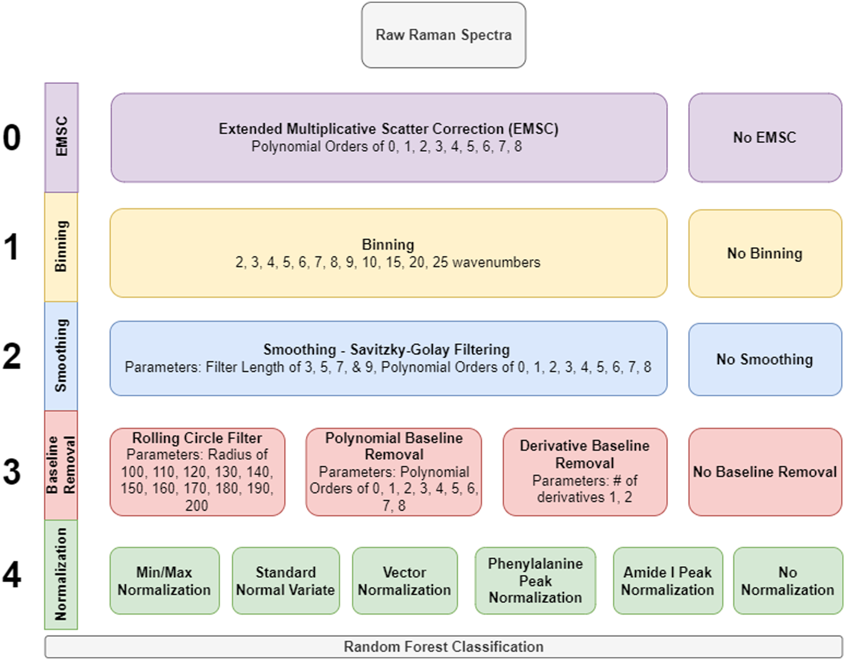

Extended Multiplicative Scatter Correction

Extended multiplicative scatter correction is a powerful method used in spectroscopy which allows for the separation of physical light-scattering effects from physical light absorbance effects.³⁰ EMSC provides a model-based approach for the correction of unwanted additive and multiplicative effects within spectra. It is used for various applications in Raman spectroscopy, from tracking metabolic products via EMSC coefficients,³¹ as a pre-processing step,^32–34 and recently enabling the removal of water from human blood serum.³⁵

Extended multiplicative scatter correction works by modelling the additive and multiplicative effects in a sample which are not indicative of the chemical fingerprint of the sample but external factors.³⁰ Briefly, for a single spectrum, x, the corrected spectrum x_cor following EMSC with a d-order polynomial can be expressed as

x_{cor} = \frac{x - \sum_{i = 0}^{d} c_{i} v_{i}}{b} = r + \frac{1}{b} e

(1)

where e is the residual part representing the spectral information of interest, r is a reference spectrum, b represents a scaling factor such that spectrum can be expressed as a sum of the reference spectrum and the residual. The reference spectrum is typically the mean of full data set, and hence in this study the chosen reference is the mean of the training set.^32,36

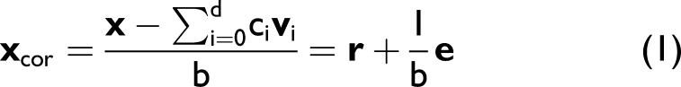
In addition to the standard EMSC model, one can include an “interferent” spectrum which can enable the specific removal of a contribution to the spectrum.³² In this work, an interferent was chosen as the empty stainless-steel substrate to isolate the serum spectra further, reducing any varying fluorescent contribution from the substrate and objective lens. EMSC is often used as the entire pre-processing protocol since it scales and models the non-chemical effects in the sample.³⁷ We also trialled EMSC as a pre-treatment prior to other methods to study the effect on classification. All implementations of EMSC were performed using the R package, “EMSC”.³⁸

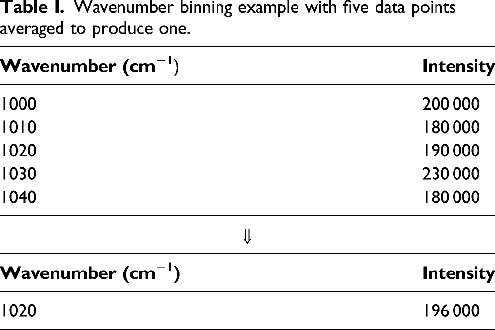
Data Binning

Data binning is the process of reducing the data points within an interval down to a single observation by averaging over a region. This method is used to minimise the effect of observational errors within a data set, and in spectral data to increase the signal-to-noise ratio. While a simple method in principle, it remains a useful tool in the chemometric arsenal.^39–41 Binning has the added benefit of reducing the data dimensionality which can decrease the computational burden on data processing. Table I shows an example of five data points binned such that they are now expressed as one data point.

Table I.

Wavenumber binning example with five data points averaged to produce one.

Wavenumber (cm⁻¹)	Intensity
1000	200 000
1010	180 000
1020	190 000
1030	230 000
1040	180 000
⇓
Wavenumber (cm ⁻¹ )	Intensity
1020	196 000

Smoothing

Spectral smoothing is the process in which noise is minimised in a data set by fitting a curve to replace the raw data thus increasing the signal-to-noise ratio. In this study, where the pre-processing sequence contains a smoothing step the Savitzky–Golay (SG) filter has been applied.⁴² SG remains prevalent in spectroscopic analysis.^40,43–45 SG functions by operating a sliding window along the data set and fitting a polynomial of order n to that window thus replacing spectra with a fitted polynomial of that window. SG is common in spectral analysis and due to having multiple tuning parameters is the only smoothing method trialled in this case.

Baseline Removal

Baseline removal is the process of removing any background contributions to the spectra from fluorescence without removing Raman features. In this study, three types of baseline removal have been trialled: rolling circle filter (RCF), polynomial baseline removal, and the use of spectra derivatives.

A rolling circle filter (RCF) is a background removal technique used in spectral pre-processing.^46–48 RCF acts as a high-pass filter for the removal of background fluorescence which works by rolling under the spectra storing the minimum distance the between the circle and the data.⁴⁶ This is repeated and evaluated for shifted windows along the spectra, resulting in a list of the minimum distance between the circumference of the circle and the spectra which are then removed from the spectra as the background contribution. The RCF removes broad features from the spectra, thus maintaining the sharp characteristic Raman peaks. The tuneable parameter with the RCF is the radius of the circle, which is typically chosen such that broad features are effectively removed and such that the circle cannot ‘roll’ into Raman peaks, hence diminishing them.

Polynomial baseline removal is a common method in pre-processing of Raman spectra.^45,49,50 A polynomial of n order models the broad background fluorescence by searching for support points beneath the spectrum and is subsequently subtracted aiming to leave behind only the chemical contributions from a sample. Polynomial baseline removal fits an n order polynomial to the spectra, aiming to remove broader features uncharacteristic of Raman while maintaining peak structures. The polynomial removal algorithm used in this study has been taken from the hyperSpec R package,⁵¹ which iteratively searches for appropriate spectral regions to fit a baseline to remove using least squares. Here the tuneable parameter is the order of the fitted polynomial.

Derivative baseline removal involves taking the derivative of Raman spectra as a high pass method of filtering and is a common technique in data pre-processing.^52–54 It can be highly effective in isolating the characteristically sharp peaks in Raman spectra from background contributions by focusing on stark changes in the spectra gradient. A drawback of using derivatives is an increase in apparent noise in a signal due to its nature of suppressing low frequency signals while enhancing high frequency signals. By taking the derivative of the measured response with respect to the wavenumber (or index), one can evaluate derivative of spectra, accentuating the maxima and minima indicative of the Raman effect. One can either take the first or second derivative to achieve this, both of which remove low frequency signals from the spectra as a high pass filter. The implementation in this study is via the Savitzky–Golay (SG) method which contains an option for derivative computation.

Normalization

Normalization aims to account for general intensity differences between spectral measurements e.g. due to relative concentration or laser power fluctuations. In this study, we trialled five types of normalization as well as an option of no normalization; min–max, min–max with the phenylalanine peak set to 1, min–max with the amide I peak set to 1, standard normal variate (SNV) and vector normalization. Min–max normalization is often used with spectroscopic data,⁵⁵ and can be focused on a particular region within the spectra to ensure a common peak is set to 1.^56–58 We used the phenylalanine peak at 1004 cm⁻¹, and the amide I peak at 1659 cm⁻¹ in human blood serum as regions to scale spectra to. Standard normal variate (SNV) is another method used in the removal of multiplicative scattering effects,⁵⁹ and as a method for scaling spectra adjusts based on the mean and standard deviation of the spectrum.^60,61 Vector normalization is also commonly used for normalization by scaling the spectra such that it sums to one.^58,62,63

Performance Comparison Using Random Forest

Each pre-processing permutation was assessed using a random forest (RF) classification algorithm.⁶⁴ Briefly, RFs build an ensemble of random decision trees, in this case 500, and uses the average result of the cohort as the final classification of the given spectra. RF is an example of a supervised learning algorithm in which the classification of a training sample is given to provide a model target, as opposed to unsupervised in which the classification of training samples is not given in model development. In RF, the number of descriptors (variables) used to determine the classification is set to the square root of the number of wavenumbers in the data set (n.b. this value may vary depending on pre-processing due to changes in data shape after pre-processing steps). These factors equate to an out-of-the-bag/default RF implementation using the R package “randomForest”, based on the original Breiman algorithm.⁶⁴ RFs are prevalent in spectroscopy,^65–67 tending to perform well without hyperparameter tuning and having the ability to extract feature importance which can be indicative of biomarkers in studies such as this. We also compare a subset of pre-processing permutations (including the top performing and bottom performing) using a support vector machine (SVM) model with linear, radial and polynomial basis functions included in the appendices to emphasise RF superiority in this context.

To train a RF model for colorectal cancer (CRC) detection, a training set containing 510 spectra from 102 patients (51 CRC, 51 control) was used with five repeat measurements each. Example raw spectra from human blood serum can be found in Jenkins et al.² An independent testing set containing 1317 spectra from 439 patients (32 CRC, 407 control) with three repeat measurements was used to evaluate the model performance for each pre-processing permutation. The distribution of CRC and controls within the independent testing set is reflective of a symptomatic patient cohort presenting in primary care and receiving referral for further investigation. Diagnosis of all patients in the training and independent testing set was confirmed via the gold standard for colorectal cancer, i.e., by colonoscopy.⁶⁸ Colonoscopy has a miss rate of up to 4%, which corresponds to a sensitivity of 96%.^69,70 100 implementations of the RF algorithm were trained and tested per pre-processing permutation with the average predicted probability of a spectra classifying as CRC or control taken. The cut-off probability for CRC/control was set to a default of majority rule (> 0.5 for either CRC or control).

When assessing the performance of each pre-processing sequence five metrics were considered, namely the sensitivity, specificity, positive predictive value (PPV), negative predictive value (NPV), accuracy and area under the receiver operator curve (AUROC). Sensitivity, specificity, PPV, NPV and accuracy are defined by different combinations of the number of true positives (TP), true negatives (TN), false positives (FP) and false negatives (FN). The relationship between the metrics in the form of a confusion matrix can be seen in Table II. The AUROC curve was included to assess the RF model capability to distinguish between CRC and non-CRC states.⁷¹ An AUROC of 0.5 indicates a model with no distinguishing capabilities. Collectively these metrics were used to produce an overall Score for a pre-processing method, given by

\begin{array}{l} Score = Sensitivity + Specificity + PPV + NPV + \\ Accuracy + AUC \end{array}

(2)

Table II.

Confusion matrix with metrics calculated based on the clinical “gold standard” actual diagnosis, and the predicted diagnosis based on the Raman measurement.

		Raman Measurement
		Negative	Positive
	Negative	TN	FN	PPV=TP / TP+FP
Gold Standard	Positive	FP	TP	NPV=TN / TN+FN
Gold Standard	Accuracy =TP + TN /TP+TN+FN+FP	Sensitivity =TP / TP+FN	Specificity =TN / TN+FP

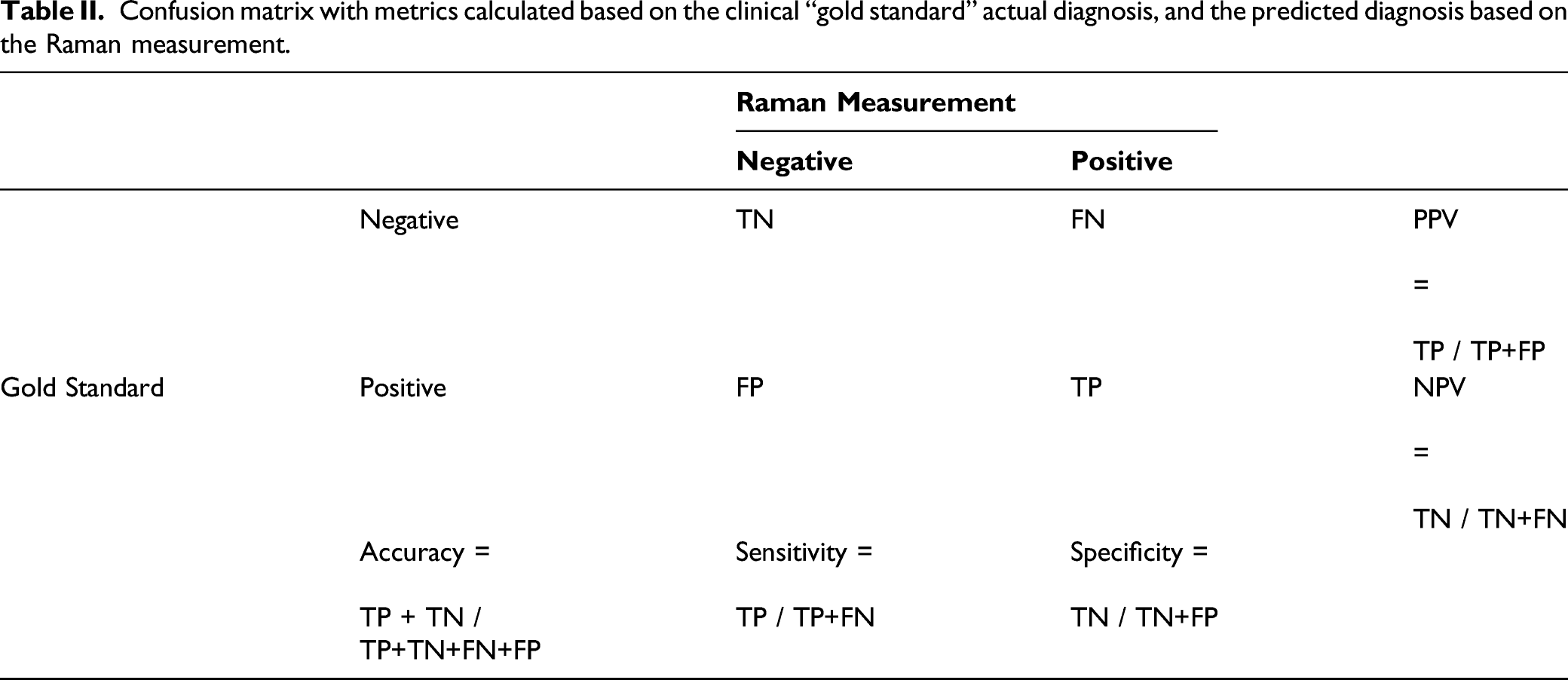
With a maximum possible value of 6. A score of 3 indicates a model with no distinguishing capability (i.e., 50%/0.5 for all values). However, prevalence of disease can affect the score, and in this study, a prevalence of ∼7% CRC meaning a score of ∼3.75 performs well.

Analysis of pre-processing permutation performance included ascertaining general trends observed and the effect individual pre-processing steps have on performance. General trend analysis included PPV NPV qualitative analysis, with a focus of the effect EMSC has on PPV and NPV on a global scale.

To select the top performing pre-processing method, the results were thresholded to obtain permutations with a sensitivity of ≥ 75% and a specificity of ≥ 50% to filter out any which do not meet this minimum requirement. In this scenario, the data are representative of a symptomatic primary care patient population with the goal of using the model as a triage tool for referrals and hence CRC prevalence in the test set is ∼ 7%. High sensitivity is favourable for a test to correctly identify CRC patients, but a trade-off with specificity (ability to correctly identify controls) must be negotiated.⁷² These thresholded permutations were then sorted to maximise the Score given in Eq. 2 to find the top performing pre-processing permutation.

Over 2.4 m pre-processing permutations in sequences shown in Fig. 1 have been tested to optimise the pre-processing methodology for RS CRC diagnosis using HPC. First, we explore the effect of each permutation on sensitivity and specificity, and a deeper analysis into the top performer using EMSC as a pre-treatment in comparison to EMSC alone. We then observe general trends for pre-processing steps on sensitivity and specificity and on the variance observed in the score metric (Eq. 2) when fixing all other pre-processing steps. The top pre-processing method is then compared to a result using no pre-processing, a standard pre-processing procedure with minimal optimisation, EMSC as a standalone method, and the worst performance we observed.

Results

Extended Multiplicative Scatter Correction Effect on Sensitivity and Specificity.

In Fig. 2, we observe a sample of ∼ 10% of the full results data set for PPV versus NPV for plotting efficiency while maintaining the top and bottom 1000 performers. Points in Fig. 2 are coloured by whether EMSC has been used as a pre-treatment or not to demonstrate general behaviour. The cone structure appears due to the “allowed” solutions given the number of patients in each category (TP, TN, FP, FN). The use of EMSC qualitatively causing PPV and NPV to fan out to the corners of the cone, unlocking regions with higher PPV results.

Figure 2.

Sensitivity vs. 1-Specificity for a sample of ∼10% of the trialled pre-processing permutations with top 1000 and bottom 1000 maintained. Spectra are coloured by whether extended multiplicative scatter correction has been used as a pre-treatment (blue) or not (red).

Top Performing Pre-processing Method

To establish the top performing pre-processing method, the full result set is thresholded as described in Methods to maximise the Score given in Eq. 2. A pre-processing ID guide is given in Table III. Table IV shows a sample of the results, with the top performing in the first row, and the worst performing in the bottom. Permutations in between show a random sample showing the variety of tested methods. The permutation achieving the highest performance is attributed to 1423-EMSC-3-B-5-S-9-1-RCF-120-norm_a achieving a sensitivity of 89.6%, specificity of 55.7%, PPV of 13.7% and NPV of 98.5%. In words, this corresponds to data pre-treated using EMSC with a third-order polynomial basis, binning of five wavenumbers, normalising to the amide peak region, smoothing with a filter length of nine and polynomial order of one, and baseline corrected using a RCF with a radius of 120. This is interesting as EMSC is typically used as an all-encompassing pre-processing method, however when used in combination with other pre-processing methods performance can be improved. In comparison, EMSC used on its own alone with a 4th order polynomial (highest achieved results for an EMSC only regime) achieved a sensitivity of 54.2%, specificity of 70.2%, PPV of 12.5%, and NPV of 95.1%. This indicates the use of other pre-processing in addition to EMSC can improve model classification. The top performing pre-processing method uses a non-standard ordering, placing normalization prior to smoothing and baseline correction. However, due to these subsequent steps scaling to the spectrum normalization coming before does not have a detrimental effect.

Table III.

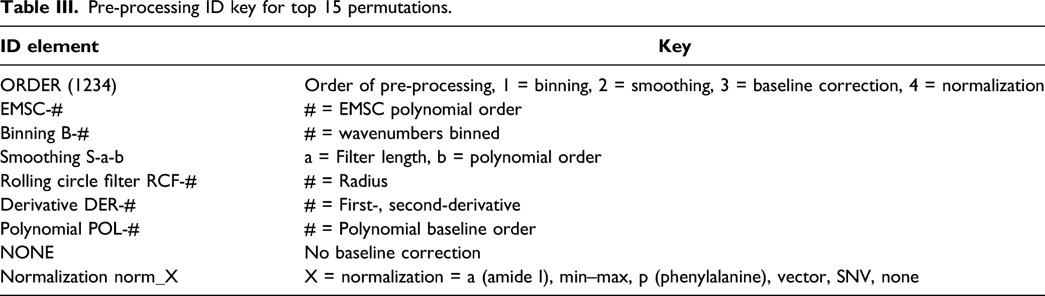
Pre-processing ID key for top 15 permutations.

ID element	Key
ORDER (1234)	Order of pre-processing, 1 = binning, 2 = smoothing, 3 = baseline correction, 4 = normalization
EMSC-#	# = EMSC polynomial order
Binning B-#	# = wavenumbers binned
Smoothing S-a-b	a = Filter length, b = polynomial order
Rolling circle filter RCF-#	# = Radius
Derivative DER-#	# = First-, second-derivative
Polynomial POL-#	# = Polynomial baseline order
NONE	No baseline correction
Normalization norm_X	X = normalization = a (amide I), min–max, p (phenylalanine), vector, SNV, none

Table IV.

Sample of results from high-performance computing pre-processing optimisations including the top performing method in the first row (1423-EMSC-3-B-5-S-9-1-RCF-120-nor-m-˙a), the worst performing pre-processing method in the bottom row (1324-6-NO-˙EMSC-2-B-S-5-RCF-200-norm-˙a), and a sample of other methods in between.

Pre-processing ID	Sensitivity	Specificity	PPV	NPV	Accuracy	AUC	Score
1423-EMSC-3-B-5-S-9-1-RCF-120-norm_a	89.6%	55.7%	13.7%	98.5%	58.1%	0.754	3.91
1324-EMSC-5-B-5-S-9-8-RCF-170-norm_minmax	62.5%	66.5%	12.8%	95.7%	66.2%	0.678	3.72
1432-EMSC-6-B-8-S-9-1-RCF-190-norm_vec	58.3%	63.9%	11.3%	95.1%	63.5%	0.645	3.57
1423-EMSC-3-B-9-S-3-5-RCF-130-norm_vec	53.1%	64.2%	10.5%	94.6%	63.4%	0.648	3.51
1423-EMSC-6-B-5-S-9-3-RCF-200-norm_snv	61.5%	57.6%	10.3%	95.0%	57.9%	0.656	3.48
1432-EMSC-7-B-2-S-7-4-RCF-110-norm_vec	56.3%	58.9%	9.7%	94.5%	58.7%	0.629	3.41
1342-EMSC-8-B-15-S-3-1-RCF-190-norm_p	54.2%	59.5%	9.5%	94.3%	59.1%	0.618	3.38
1234-EMSC-7-B-6-S-7-0-POL-4-norm_minmax	55.2%	57.7%	9.3%	94.2%	57.5%	0.616	3.36
1234-EMSC-7-B-6-S-5-5-DER-1-norm_minmax	66.7%	51.0%	9.7%	95.1%	52.1%	0.596	3.34
1324-6-NO_EMSC-2-B-S-5-RCF-200-norm_a	51.0%	30.5%	5.5%	88.8%	32.0%	0.402	2.48

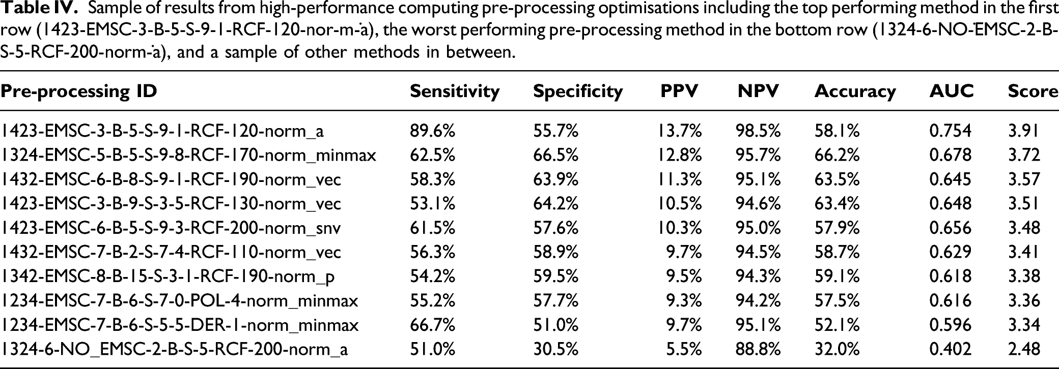
When focusing on only the top 100 pre-processing permutations, the Score metric varies by at most by 0.1, that is, 10% in total across all performance metrics. Only one pre-processing method arises in the majority ( $> 50 %$ in the top 100) of cases; RCF with 88/100 permutations. The remaining 12/100 baseline correction are polynomial baseline correction with no derivative arising in the top 100. No other pre-processing method/variable combination see such a large proportion dominating the top 100. Notable mentions include low order polynomials for smoothing (0–3) with 70/100 in the top 100, with filter lengths of seven and nine in 84/100 permutations. In addition, high order polynomial orders (seven and eight) for EMSC appear to be more favourable with this data set with 52/100 of the top 100 permutations.

General Trends

Figure 3 demonstrates a random sample of ∼10% of pre-processing methods trialled and their corresponding sensitivity and specificity, in this case, coloured by baseline correction technique. The use of the derivative for baseline correction of spectra tends to perform with low PPV, with only a few permutations appearing more centrally in the cone. RCF and polynomial baseline removal dominate the thresholded region which focuses on results with sensitivity ≥ 75% and specificity ≥ 50%, however a small number of derivative implementations also perform in this region too.

Figure 3.

Pre-processing permutations trialled coloured by baseline correction algorithm. The plot contains ∼ 10% of the full cohort of pre-processing permutations for plotting efficiency. Zoomed in region is thresholded with sensitivity ≥ 75% and an specificity ≥ 50% and contains all data points that meet this criteria (∼800 000).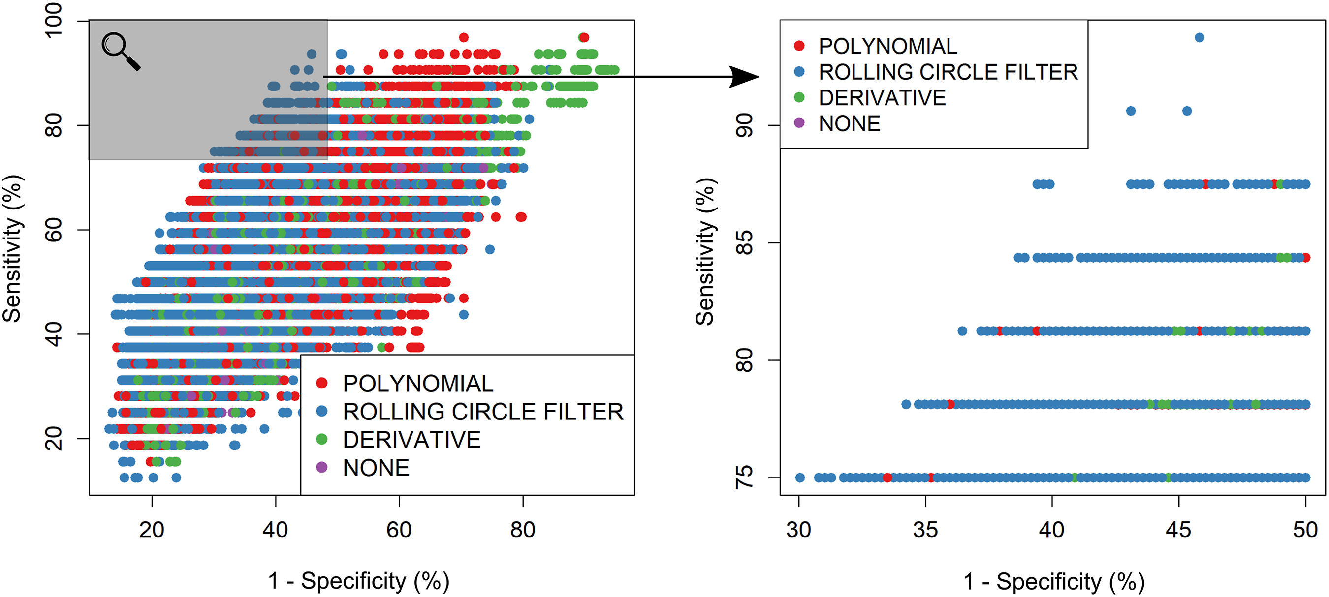

In Fig. 4, we observed the standard deviation in the score (Eq. 2) for each pre-processing step or ordering when all other steps are fixed, isolating the change in score to only one step. This is computed by grouping together pre-processing IDs with the step we wish to vary not included and hence computing the standard deviation of the score in the group. EMSC affects the score-value the highest on average, which is to be expected due to the nature of EMSC modelling spectra to a reference, and hence altering the raw spectra immediately. Baseline correction and ordering of pre-processing then have the next highest effect on Score on average, and notably the order of pre-processing sees some large outlying effects on scores. Binning spectra also causes significant outliers, with deviations up to 0.4 in score metric. Normalization typically has a small effect on average, however, does have large outliers which is overwhelmingly due to the normalization step coming before other pre-processing steps. Smoothing has the smallest effect on average which may be due to the type of data trialled in this study, that is, Raman spectra from human blood serum where the average of the training set is 31 ± 24 computed from the mean intensity divided by standard deviation between replicate spectra.⁷³ An example of serum spectra with varying SNR is shown in the Supplemental Material.

Figure 4.

Variance in the Score when altering a single step in the process while fixing all other parameters. Smoothing has the smallest effect when fixing other parameters and the ordering sees the largest spread.

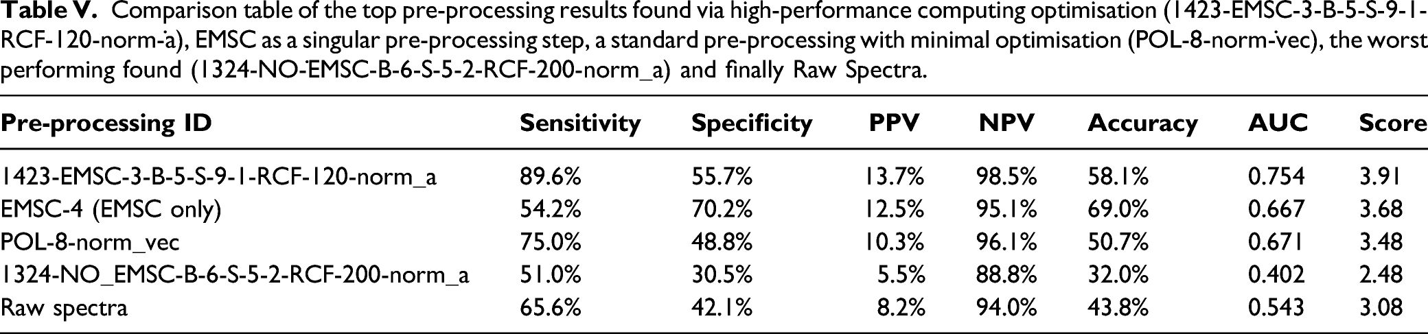
The best performing pre-processing method is compared to no pre-processing, EMSC alone, a standard minimally optimised pre-processing (polynomial baseline removal with vector normalization) and the worst performing method as observed in Table V. Optimised pre-processing via HPC enables improvements of up to an additional 14.6% sensitivity compared to a minimal optimisation, which can be seen comparing the first and final row in Table V. Up to 24.0% improvement in sensitivity is seen compared to no pre-processing.

Table V.

Comparison table of the top pre-processing results found via high-performance computing optimisation (1423-EMSC-3-B-5-S-9-1-RCF-120-norm-˙a), EMSC as a singular pre-processing step, a standard pre-processing with minimal optimisation (POL-8-norm-˙vec), the worst performing found (1324-NO-˙EMSC-B-6-S-5-2-RCF-200-norm_a) and finally Raw Spectra.

Pre-processing ID	Sensitivity	Specificity	PPV	NPV	Accuracy	AUC	Score
1423-EMSC-3-B-5-S-9-1-RCF-120-norm_a	89.6%	55.7%	13.7%	98.5%	58.1%	0.754	3.91
EMSC-4 (EMSC only)	54.2%	70.2%	12.5%	95.1%	69.0%	0.667	3.68
POL-8-norm_vec	75.0%	48.8%	10.3%	96.1%	50.7%	0.671	3.48
1324-NO_EMSC-B-6-S-5-2-RCF-200-norm_a	51.0%	30.5%	5.5%	88.8%	32.0%	0.402	2.48
Raw spectra	65.6%	42.1%	8.2%	94.0%	43.8%	0.543	3.08

Conclusion

Choice of pre-processing in RS is a task with many variables from instrumentation, to sample type, to task at hand and a lack of consensus in the community leads to time-consuming trial and error optimisations. In this contribution, we have explored the use of HPC for the task of optimising spectral pre-processing with a disease diagnostic aim.

Over 2.4 million different permutations of pre-processing have been trialled to understand the effect of reordering pre-processing, using EMSC, binning of wavenumbers, SG smoothing, baseline correction, and normalization. We have found EMSC in conjunction with other pre-processing steps to obtain the highest performance with sensitivity of 89.6%, specificity of 55.7%, PPV of 13.7% and NPV of 98.5% in comparison to using EMSC as a standalone pre-processing achieving sensitivity of 54.2%, specificity of 70.2%, PPV of 12.5%, and NPV of 95.1%. EMSC is typically used as a comprehensive pre-processing technique which we find to improve performance when used in conjunction with other pre-processing techniques to smooth, bin, baseline correct, and normalise. EMSC is reliant on representative reference spectra to model all other spectra to. In this study, the reference spectra have been set to average spectra, a common choice. Other options have been studied, however it has been noted the reference choice is not important but must remain consistent.⁷⁴ In a regime using minimal pre-processing optimisation, a sensitivity of 75.0%, specificity of 48.8%, PPV of 10.3% and NPV of 96.1% is achieved. However, due to the small training set used in development, the top pre-processing established may be finding a non-scalable solution. Future work will re-optimise pre-processing with a larger training set.

While this study is specifically targeted to optimise model performance for diseased and non-diseased state classification, the aim is to demonstrate a methodology for approaching similar tasks where consensus has not been met in the community. Optimal pre-processing may vary depending on task, instrumentation (Raman instrument, objective, laser, etc.) and on sample/substrate and hence should be repeated for new tasks.

In this study we have exploited HPC, however it is possible to achieve significant improvements in model performance using local scripts for optimisation of pre-processing. We cover a wide range of pre-processing parameters to understand the edge cases but searching in a smaller parameter space can still be of benefit, particularly if paired with parallelisation of one’s local computer.

In the case where a supercomputer is not available for use, the authors have the following recommendations; ordering of pre-processing is not important as long as the baseline correction algorithm is scaling to the data. Smoothing may be skipped, or just fixed if it is necessary for the data set due to the small effect over many different parameters. Binning with large wavenumbers can produce a large variance between different permutations, hence keeping this below 10 should be sufficient for systems with similar spectral resolution (∼0.5 cm⁻¹).

High-performance computing offers a powerful tool for data processing and optimisation, in this case utilised to optimise RS pre-processing of blood serum samples for disease detection. Harnessing supercomputing capabilities unlocks the ability to generate and analyse large quantities of data rapidly which can enable optimisation of computations with ease. While this study has focused on a Raman data set for disease detection, the methodology set out can be applied to other applications and other spectra-type data sets for improved model classification ability or other relevant measures of performance.

Supplemental Material

sj-pdf-1-asp-10.1177_00037028221088320 – Supplemental Material for Optimised Pre-Processing of Raman Spectra for Colorectal Cancer Detection Using High-Performance Computing

Supplemental Material, sj-pdf-1-asp-10.1177_00037028221088320 for Optimised Pre-Processing of Raman Spectra for Colorectal Cancer Detection Using High-Performance Computing by Freya E. R. Woods, Cerys A. Jenkins, Rhys A. Jenkins, Susan Chandler, Dean A. Harris and Peter R. Dunstan in Applied Spectroscopy

Footnotes

Declaration of Conflicting Interests

The author(s) declared the following potential conflicts of interest with respect to the research, authorship, and/or publication of this article: PRD, DAH and CAJ declare their involvement in CanSense Ltd, a recently incorporated cancer diagnosis spin-out company from Swansea University (company no. 11367637).

Funding

The author(s) disclosed receipt of the following financial support for the research, authorship, and/or publication of this article: This work has been funded through a PhD studentship by Cancer Research Wales (Registered Charitable Incorporated Organisation Number: 1167290) to whom we are grateful for continued support. The authors wish to acknowledge the support of the Supercomputing Wales project, which is part-funded by the European Regional Development Fund (ERDF) via the Welsh Government.

ORCID iDs

Freya E. R. Woods

Susan Chandler

Supplemental Material

All supplemental material mentioned in the text is available in the online version of the journal.

References

Gardiner

Graves

. Practical Raman Spectroscopy. Berlin, Heidelberg: Springer, 1989. doi: 10.1007/978-3-642-74040-4.

Jenkins

C.A.

Jenkins

R.A.

Pryse

M.M.

Welsby

K.A.

, et al. “A High-Throughput Serum Raman Spectroscopy Platform and Methodology for Colorectal Cancer Diagnostics”. Analyst. 2018. 143(24): 6014–6024. doi: 10.1039/C8AN01323C.

Sohail

Khan

Ullah

Qureshi

S.A.

, et al. “Analysis of Hepatitis C Infection Using Raman Spectroscopy and Proximity Based Classification in the Transformed Domain”. Biomed. Opt. Express. 2018. 9(5): 2041. doi: 10.1364/BOE.9.002041

Khan

Ullah

Shahzad

Anbreen

, et al. “Analysis of Tuberculosis Disease Through Raman Spectroscopy and Machine Learning”. Photodiagn. Photodyn. Ther. 2018. 24: 286–291. doi: 10.1016/J.Pdpdt.2018.10.014.

Khan

Ullah

Khan

Wahab

, et al. “Analysis of Dengue Infection Based on Raman Spectroscopy and Support Vector Machine (SVM)”. Biomed. Opt. Express. 2016. 7(6): 2249. doi: 10.1364/Boe.7.002249.

Woods

F.E.

Chandler

Sikora

Harford

, et al. “An Observational Cohort Study to Evaluate the Use of Serum Raman Spectroscopy in a Rapid Diagnosis Centre Setting”. Clin. Spectrosc. 2022. Vol. 4. doi: 10.1016/J.Clispe.2022.100020.

Aubertin

Trinh

V.Q.

Jermyn

Baksic

, et al. “Mesoscopic Characterization of Prostate Cancer Using Raman Spectroscopy: Potential for Diagnostics and Therapeutics”. BJU Int. 2018. 122(2): 326–336. doi: 10.1111/Bju.14199.

Ding

Cao

Dupont

A.W.

Scott

L.D.

, et al. “Discrimination of Inflammatory Bowel Disease Using Raman Spectroscopy and Linear Discriminant Analysis Methods". Paper presented at: Biomedical Vibrational Spectroscopy 2016: Advances in Research and Industry. San Francisco, California; 13-14 February 2016. 97040W. doi: 10.1117/12.2225299.

Zheng

Qing

Wang

Lü

, et al. “Diagnosis of Cervical Squamous Cell Carcinoma and Cervical Adenocarcinoma Based on Raman Spectroscopy and Support Vector Machine” Photodiagn. Photodyn. Ther. 2019. 27: 156–161. doi: 10.1016/J.Pdpdt.2019.05.029.

10.

Teh

S.K.

Zheng

K.Y.

Teh

, et al. “Near-Infrared Raman Spectroscopy for Early Diagnosis and Typing of Adenocarcinoma in the Stomach”. Brit. J. Surgery. 2010. 97(4): 550–557. doi: 10.1002/Bjs.6913.

11.

Potter

Tomas

Elson

J.L.

, et al. “A New Approach to Find Biomarkers in Chronic Fatigue Syndrome/Myalgicencephalomyelitis (CFS/ME) by Single-Cell Raman Microspectroscopy”. Analyst 2019. 144(3): 913–920. doi: 10.1039/C8an01437j.

12.

Becker-Putsche

Bocklitz

Clement

Rösch

Popp

. “Toward Improving Fine Needle Aspiration Cytology by Applying Raman Microspectroscopy”. J. Biomed. Opt. 2013. 18(4): 047001. doi: 10.1117/1.Jbo.18.4.047001.

13.

Pyrgiotakis

Kundakcioglu

O.E.

Pardalos

P.M.

Moudgil

B.M.

. “Raman Spectroscopy and Support Vector Machines for Quick Toxicological Evaluation of Titania Nanoparticles”. J. Raman Spectrosc. 2011. 42(6): 1222–1231. doi: 10.1002/Jrs.2839.

14.

Byrne

H.J.

Baranska

Puppels

G.J.

Stone

, et al. “Spectropathology for the Next Generation: Quo Vadis?” Analyst. 2015. 140(7): 2066–2073. doi: 10.1039/C4AN02036G.

15.

Ullah

Khan

Ali

Chaudhary

I.I.

, et al. “A Comparative Study of Machine Learning Classifiers for Risk Prediction of Asthma Disease”. Photodiagn. Photodyn. Ther. 2019. 28: 292–296. doi: 10.1016/J.Pdpdt.2019.10.011.

16.

Khan

Ullah

Khan

Ashraf

, et al. “Analysis of Hepatitis B Virus Infection in Blood Sera Using Raman Spectroscopy and Machine Learning”. Photodiagn. Photodyn. Ther. 2018. 23: 89–93. doi: 10.1016/J.Pdpdt.2018.05.010.

17.

Chen

P.H.C.

Liu

Peng

. “How to Develop Machine Learning Models for Healthcare”. Nat. Mat. 2019. 18(5): 410–414. doi: 10.1038/S41563-019-0345-0.

18.

Shreve

A.P.

Cherepy

N.J.

Mathies

R.A.

. “Effective Rejection of Fluorescence Interference in Raman Spectroscopy Using a Shifted Excitation Difference Technique”. Appl. Spectrosc. 1992. 46(4): 707–711. doi: 10.1366/0003702924125122.

19.

De Luca

A.C.

Mazilu

Riches

Herrington

C.S.

Dholakia

. “Online Fluorescence Suppression in Modulated Raman Spectroscopy”. Anal. Chem. 2010. 82(2): 738–745. doi: 10.1021/Ac9026737.

20.

Heraud

Wood

B.R.

Beardall

McNaughton

. “Effects of Pre-Processing of Raman Spectra on in Vivo Classification of Nutrient Status of Microalgal Cells”. J. Chemom. 2006. 20(5): 193–197. doi: 10.1002/Cem.990.

21.

Lasch

. “Spectral Pre-Processing for Biomedical Vibrational Spectroscopy and Microspectroscopic Imaging”. Chemom. Intell. Lab. Syst. 2012. 117: 100–114. doi: 10.1016/J.Chemolab.2012.03.011.

22.

Guo

Popp

Bocklitz

. “Chemometric Analysis in Raman Spectroscopy from Experimental Design to Machine Learning -Based Modeling”. Nat. Protoc. 2021 16:12 2021. 16(12): 5426–5459. doi: 10.1038/S41596-021-00620-3.

23.

Bocklitz

Walter

Hartmann

Rösch

Popp

. “How to Pre-Process Raman Spectra for Reliable and Stable Models?” Anal. Chim. Acta. 2011. 704(1-2): 47–56. doi: 10.1016/J.Aca.2011.06.043.

24.

Guo

Bocklitz

Popp

. Optimization of Raman Spectrum Baseline Correction in Biological Application”. Analyst. 2016. 141(8): 2396–2404. doi: 10.1039/C6an00041j.

25.

Storey

E.E.

Helmy

A.S.

. Optimized Preprocessing and Machine Learning for Quantitative Raman Spectroscopy in Biology”. J. Raman Spectrosc. 2019. 50(7): 958–968. doi: 10.1002/Jrs.5608.

26.

Butler

H.J.

Smith

B.R.

Fritzsch

Radhakrishnan

, et al. “Optimised Spectral Pre-Processing for Discrimination of Biofluids via ATR-FTIR Spectroscopy”. Analyst. 2018. 143(24): 6121–6134. doi: 10.1039/C8AN01384E.

27.

Misra

. “Machine Learning Assisted Segmentation of Scanning Electron Microscopy Images of Organic-Rich Shales with Feature Extraction and Feature Ranking”. In: Misra

, editors. Machine Learning for Subsurface Characterization. Cambridge, Massachusetts: Elsevier, 2020. Chap. 10, Pp. 289–314. doi: 10.1016/B978-0-12-817736-5.00010-7.

28.

Supercomputing Wales. “Supercomputing Wales Portal: Resources and Support for Users of the Supercomputing Wales Services. About Sunbird". https://portal.supercomputing.wales/index.php/about-sunbird/ [accessed Mar 23 2022].

29.

Woods

F.E.

Dunstan

P.R.

. “PPRaman: A Package to Handle Pre-Processing of Raman Datasets in R”. 2021. https://github.com/ferwoods/ppraman [accessed Mar 23 2022].

30.

Martens

Stark

. “Extended Multiplicative Signal Correction and Spectral Interference Subtraction: New Preprocessing Methods for Near Infrared Spectroscopy”. J. Pharm. Biomed. Anal. 1991. 9(8): 625–635. doi: 10.1016/0731-7085(91)80188-F.

31.

De Gelder

De Gussem

Vandenabeele

Moens

. “Reference Database of Raman Spectra of Biological Molecules”. J. Raman Spectrosc. 2007. 38(9): 1133–1147. doi: 10.1002/Jrs.1734.

32.

Liland

K.H.

Kohler

Afseth

N.K.

. “Model-Based Preprocessing in Raman Spectroscopy of Biological Samples”. J. Raman Spectrosc. 2016. 47(6): 643–650. doi: 10.1002/Jrs.4886.

33.

Lafhal

Vanloot

Bombarda

Valls

, et al. “Raman Spectroscopy for Identification and Quantification Analysis of Essential Oil Varieties: A Multivariate Approach Applied to Lavender and Lavandin Essential Oils”. J. Raman Spectrosc. 2015. 46(6): 577–585. doi: 10.1002/Jrs.4697.

34.

Troein

Siregar

Beeck

M.O.D.

Peterson

, et al. “OCTAVVS: A Graphical Toolbox for High-Throughput Preprocessing and Analysis of Vibrational Spectroscopy Imaging Data”. Methods and Protocols 2020. 3(2): 34. doi: 10.3390/Mps3020034.

35.

Parachalil

D.R.

Bruno

Bonnier

Blasco

, et al. “Raman Spectroscopic Screening of High and Low Molecular Weight Fractions of Human Serum”. Analyst. 2019. 144(14): 4295–4311. doi: 10.1039/C9an00599d.

36.

Skogholt

Liland

K.H.

Indahl

U.G.

. Preprocessing of Spectral Data in the Extended Multiplicative Signal Correction Framework Using Multiple Reference Spectra”. J. Raman Spectrosc. 2019. 50(3): 407–417. doi: 10.1002/Jrs.5520.

37.

Gautam

Vanga

Ariese

Umapathy

. “Review of Multidimensional Data Processing Approaches for Raman and Infrared Spectroscopy”. EPJ Tech. Instrum. 2015. 2(1). doi: 10.1140/Epjti/S40485-015-0018-6.

38.

Liland

K.H.

Indahl

U.G.

. EMSC: Extended Multiplicative Signal Correction. https://cran.r-project.org/web/packages/emsc/index.html [accessed Mar 23 2022].

39.

Lieber

C.A.

Mahadevan-Jansen

. “Automated Method for Subtraction of Fluorescence from Biological Raman Spectra”. Appl. Spectrosc. 2003. 57(11): 1363–1367. doi: 10.1366/000370203322554518.

40.

Kanter

E.M.

Majumder

Vargis

Robichaux-Viehoever

, et al. “Multiclass Discrimination of Cervical Precancers Using Raman Spectroscopy”. J. Raman Spectrosc. 2009. 40(2): 205–211. doi: 10.1002/Jrs.2108.

41.

Webb-Robertson

B.J.M.

Bailey

V.L.

Fansler

S.J.

Wilkins

M.J.

Hess

N.J.

. “Spectral Signatures for the Classification of Microbial Species Using Raman Spectra”. Anal. Bioanal. Chem. 2012. 404(2): 563–572. doi: 10.1007/S00216-012-6152-Y.

42.

Savitzky

Golay

M.J.E.

“Smoothing and Differentiation of Data by Simplified Least Squares Procedures”. Anal. Chem. 1964. 36(8): 1627–1639. doi: 10.1021/Ac60214a047.

43.

Romero-Torres

Pérez-Ramos

J.D.

Morris

K.R.

Grant

E.R.

. “Raman Spectroscopy for Tablet Coating Thickness Quantification and Coating Characterization in the Presence of Strong Fluorescent Interference”. J. Pharm. Biomed. Anal. 2006. 41(3): 811–819. doi: 10.1016/J.Jpba.2006.01.033.

44.

Di Anibal

C.V.

Marsal

L.F.

Callao

M.P.

Ruisánchez

. “Surface Enhanced Raman Spectroscopy (SERS) and Multivariate Analysis As a Screening Tool for Detecting Sudan I Dye in Culinary Spices”. Spectrochim. Acta, Part A. 2012. 87: 135–141. doi: 10.1016/J.Saa.2011.11.027.

45.

Gouvinhas

Machado

Carvalho

de Almeida

J.M.M.M.

Barros

A.I.R.N.A.

. “Short Wavelength Raman Spectroscopy Applied to the Discrimination and Characterization of Three Cultivars of Extra Virgin Olive Oils in Different Maturation Stages”. Talanta. 2015. 132: 829–835.doi: 10.1016/J.Talanta.2014.10.042.

46.

Brandt

N.N.

Brovko

O.O.

Chikishev

A.Y.

Paraschuk

O.D.

. “Optimization of the Rolling-Circle Filter for Raman Background Subtraction”. Appl. Spectrosc. 2006. 60(3):288–293. doi: 10.1366/000370206776342553.

47.

Moore

D.S.

Scharff

R.J.

. “Portable Raman Explosives Detection”. Anal. Bioanal. Chem. 2009. 393(6-7): 1571–1578. doi: 10.1007/S00216-008-2499-5.

48.

S.K.

Yoo

S.J.

Jeong

D.H.

Lee

J.M.

. “Real-Time Estimation of Glucose Concentration in Algae Cultivation System Using Raman Spectroscopy”. Biores. Technol. 2013. 142: 131–137. doi: 10.1016/J.Biortech.2013.05.008.

49.

Dong

Zhang

Wang

. “Quantitative Analysis of Adulteration of Extra Virgin Olive Oil Using Raman Spectroscopy Improved by Bayesian Framework Least Squares Support Vector Machines”. Anal. Methods. 2012. 4(9):2772–2777. doi: 10.1039/C2ay25431j.

50.

C.S.

Jean

Hogan

C.A.

Blackmon

, et al. “Rapid Identification of Pathogenic Bacteria Using Raman Spectroscopy and Deep Learning”. Nat. Commun. 2019. 10(1). doi: 10.1038/S41467-019-12898-9.

51.

Beleites

Sergo

. “Hyperspec: A Package to Handle Hyperspectral Data Sets in R”. https://github.com/cbeleites/hyperspec [accessed Mar 23 2022].

52.

Himmelsbach

D.S.

Barton

F.E.

McClung

A.M.

Champagne

E.T.

. “Protein and Apparent Amylose Contents of Milled Rice by NIR-FT/Raman Spectroscopy”. Cereal Chem. J. 2001. 78(4): 488–492. doi: 10.1094/CCHEM.2001.78.4.488.

53.

Uysal

R.S.

Boyaci

I.H.

Genis

H.E.

Tamer

. “Determination of Butter Adulteration with Margarine Using Raman Spectroscopy”. Food Chem. 2013. 141(4): 4397–4403. doi: 10.1016/J.Foodchem.2013.06.061.

54.

Boyaci

I.H.

Temiz

T.H.

Uysal

R.S.

Velioğlu

H.M.

, et al. “A Novel Method for Discrimination of Beef and Horsemeat Using Raman Spectroscopy”. Food Chem. 2014. 148: 37–41. doi: 10.1016/J.Foodchem.2013.10.006.

55.

Conroy

Ryder

A.G.

Leger

M.N.

Hennessey

Madden

M.G.

. “Qualitative and Quantitative Analysis of Chlorinated Solvents Using Raman Spectroscopy and Machine Learning”. Proc. SPIE 5826, Opto-Ireland 2005: Optical Sensing and Spectroscopy. 5826: 131. doi: 10.1117/12.605056.

56.

O'Grady

Dennis

A.C.

Denvir

McGarvey

J.J.

Bell

S.E.

. “Quantitative Raman Spectroscopy of Highly Fluorescent Samples Using Pseudo Second Derivatives and Multivariate Analysis”. Anal. Chem. 2001. 73(9): 2058–2065. doi: 10.1021/Ac0010072.

57.

Mazurek

Szostak

. “Quantitative Determination of Captopril and Prednisolone in Tablets by FT-Raman Spectroscopy”. J. Pharm. Biomed. Anal. 2006. 40(5): 1225–1230. doi: 10.1016/J.Jpba.2005.03.047.

58.

Schmid

Rösch

Krause

Harz

, et al. “Gaussian Mixture Discriminant Analysis for the Single-Cell Differentiation of Bacteria Using Micro-Raman Spectroscopy”. Chemom. Intell. Lab. Syst. 2009. 96(2): 159–171. doi: 10.1016/J.Chemolab.2009.01.008.

59.

Barnes

R.J.

Dhanoa

M.S.

Lister

S.J.

. “Standard Normal Variate Transformation and De-Trending of Near-Infrared Diffuse Reflectance Spectra”. Appl. Spectrosc. 1989. 43(5): 772–777. doi: 10.1366/0003702894202201.

60.

Romero-Torres

Pérez-Ramos

J.D.

Morris

K.R.

Grant

E.R.

. “Raman Spectroscopic Measurement of Tablet-to-Tablet Coating Variability”. J. Pharm. Biomed. Anal. 2005. 38(2): 270–274. doi: 10.1016/J.Jpba.2005.01.007.

61.

Kachrimanis

Braun

D.E.

Griesser

U.J.

. “Quantitative Analysis of Paracetamol Polymorphs in Powder Mixtures by FT-Raman Spectroscopy and PLS Regression”. J. Biomed. Pharm. Biomed. Anal. 2007. 43(2): 407–412. doi: 10.1016/J.Jpba.2006.07.032.

62.

Driskell

J.D.

Seto

A.G.

Jones

L.P.

Jokela

Dluhy

R.A.

, et al. “Rapid Micro-RNA (Mirna) Detection and Classification Via Surface-Enhanced Raman Spectroscopy (SERS)”. Biosens. Bioelectron. 2008. 24(4): 917–922. doi: 10.1016/J.Bios.2008.07.060.

63.

Neugebauer

Bocklitz

Clement

J.H.

Krafft

Popp

. “Towards Detection and Identification of Circulating Tumour Cells Using Raman Spectroscopy”. Analyst. 2010. 135(12): 3178–3182. doi: 10.1039/C0an00608d.

64.

Breiman

. “ST4_Method_Random_Forest“. Mach. Learn. 2001. 45(1): 5–32. doi: 10.1017/CBO9781107415324.004.

65.

Amjad

Ullah

Khan

Bilal

Khan

. “Raman Spectroscopy-Based Analysis of Milk Using Random Forest Classification”. Vib. Spectrosc. 2018. 99: 124–129. doi: 10.1016/J.Vibspec.2018.09.003. URL doi: 10.1016/J.Vibspec.2018.09.003.

66.

Khan

Ullah

Khan

Sohail

, et al. “Random Forest-Based Evaluation of Raman Spectroscopy for Dengue Fever Analysis”. Appl. Spectrosc. 2017. 71(9): 2111–2117. doi: 10.1177/0003702817695571.

67.

Magee

N.D.

Beattie

J.R.

Carland

Davis

, et al. “Raman Microscopy in the Diagnosis and Prognosis of Surgically Resected Nonsmall Cell Lung Cancer”. J. Biomed. Opt. 2010. 15(2): 026015. doi: 10.1117/1.3323088.

68.

Rees

C.J.

Thomas Gibson

Rutter

M.D.

Baragwanath

, et al. “UK Key Performance Indicators and Quality Assurance Standards for Colonoscopy”. Brit. Soc. Gastroenterol. 2019. https://www.bsg.org.uk/wp-content/uploads/2019/12/uk-key-performance-indicators-and-quality-assurance-standards-for-colonoscopy-1.pdf [accessed Mar 23 2022].

69.

Bressler

Paszat

L.F.

Chen

Rothwell

, et al. “Rates of New Or Missed Colorectal Cancers After Colonoscopy and Their Risk Factors: A Population-Based Analysis”. Gastroenterol. 2007. 132(1): 96–102. doi: 10.1053/J.GASTRO.2006.10.027.

70.

Than

Witherspoon

Shami

Patil

Saklani

. “Diagnostic Miss Rate for Colorectal Cancer: An Audit”. Ann. Gastroenterol. 2015. 28(1): 94–98.

71.

Fawcett

. “An Introduction to ROC Analysis”. Pattern Recognit. Lett. 2006. 27(8): 861–874. doi: 10.1016/J.Patrec.2005.10.010.

72.

Lalkhen

A.G.

McCluskey

. “Clinical Tests: Sensitivity and Specificity”. BJA CEACCP. 2008. 8(6): 221–223. doi: 10.1093/Bjaceaccp/Mkn041.

73.

McCreery

R.L.

. "Signal-to-Noise in Raman Spectroscopy". Raman Spectroscopy for Chemical Analysis. New York: John Wiley and Sons, 2000. Ch. 4, Pp. 49–71. doi: 10.1002/0471721646.ch4.

74.

Kohler

Afseth

N.K.

Martens

. “Chemometrics in Biospectroscopy”. In: Li-Chan

E.Y.C.

Chalmers

J.M.

Griffiths

P.R.

, Editor. Applications of Vibrational Spectroscopy in Food Science. Chichester, UK: John Wiley and Sons, 2010. Pp. 89–106. doi: 10.1002/0470027320.S8937.

Supplementary Material

Please find the following supplemental material available below.

For Open Access articles published under a Creative Commons License, all supplemental material carries the same license as the article it is associated with.

For non-Open Access articles published, all supplemental material carries a non-exclusive license, and permission requests for re-use of supplemental material or any part of supplemental material shall be sent directly to the copyright owner as specified in the copyright notice associated with the article.

0.00 MB

0.47 MB